Efficient Prediction of Quasi-Phase Equilibrium in KKS Phase Field Model via Grey Wolf-Optimized Neural Network

1  Introduction

In recent years, significant progress has been made in understanding phase transformations in metals and alloys. While achieving complete equilibrium requires each phase to attain the configuration of minimum free energy and comply with Gibbs’ phase rule, real-world material systems typically exist in a quasi-equilibrium state due to factors such as elemental diffusion, interfacial energy, and structural defects [1]. Under these influences, the phase composition, distribution, and morphology remain relatively stable over certain time scales, despite not being fully equilibrated. To characterize microstructural evolution under such quasi-equilibrium conditions, modern phase-field models employ coupled partial differential equations that integrate temperature fields, concentration fields, and phase-field order parameters. These models have proven effective in capturing both microscopic and macroscopic solidification phenomena in metallic systems [2–5]. For instance, Wang et al. [6] successfully predicted microstructural evolution in alloys using phase-field simulations. Boettinger et al. [7] modeled phase transitions at various temperatures, providing a solid theoretical framework for understanding microstructural dynamics during solidification. Tourret et al. [8] further demonstrated the method’s effectiveness in predicting material behavior and structural transformations.

Despite their widespread use, the development and application of phase-field models often depend on extensive experimental datasets and intricate mathematical formulations, resulting in substantial computational overhead and heightened sensitivity to input parameters. These limitations can hinder the accurate representation of global microstructural behavior and compromise predictive reliability. Particularly in the context of complex multicomponent alloy systems, traditional approaches such as CALPHAD–although known for their high predictive fidelity [9]–are constrained by long computation times and a strong dependence on thermodynamic databases. Such limitations reduce their practicality in high-frequency iterative tasks, including multi-objective optimization. Among these systems, the Al–Cu–Mg ternary alloy stands out as a lightweight structural material of critical industrial relevance [10], extensively employed in aerospace and transportation due to its superior strength and corrosion resistance. During solidification, the alloy exhibits intricate phenomena such as dendritic growth, eutectic reactions, and precipitation of strengthening phases. These microstructural features are intimately linked to its mechanical performance and exemplify a typical solid-liquid coexistence regime [11–13]. Notably, the coupled evolution of solid and liquid phases–driven by interdendritic liquid redistribution and multicomponent solute segregation–plays a pivotal role in shaping the final morphology and elemental distribution, thereby exerting a profound influence on the resulting mechanical properties.

To enhance the predictive accuracy and computational efficiency of phase-field models for multicomponent alloys, recent research has increasingly focused on integrating machine learning techniques to optimize and improve modeling performance [14–17]. Jaliliantabar et al. [18] used deep learning techniques to study the thermal conduction behavior in phase change materials. They trained neural networks to predict the thermal conductivity of materials in different phase change states and applied this to the efficient design and optimization of phase change materials. This method significantly reduced the time required for experiments and simulations, but still faces issues of stability and accuracy of neural networks in complex phase change processes. Hu et al. [19] proposed using neural networks for phase field simulation to replace traditional dynamic methods. However, the training process of this method requires a significant amount of computational resources and time, especially when applied to large systems. Fuhr et al. [20] proposed a deep learning-based materials design method that combines neural networks and high-throughput computing to achieve rapid predictions of material properties. This method trains a neural network model to learn the relationship between the structure and properties of materials, thus reducing the resources and time required by traditional experimental and computational methods. Although this method has made significant progress in predicting material properties, the training iterations of the neural network model still require a large amount of computational resources, especially when dealing with complex material systems. Fan et al. [21] proposed a combination of phase field simulation and deep learning models to accelerate the simulation of the grain growth process. They utilized deep learning methods to learn the dynamic behavior of grain boundaries, achieving faster and more accurate simulations of grain growth. Although using deep learning generative models to accelerate grain growth simulations has made some progress, this method is still limited by the accuracy and stability of the generative models.

These studies indicate that the application of machine learning in materials science has made significant progress, but still faces some challenges. Traditional machine learning and neural networks face issues such as getting trapped in local optima and slow convergence during the optimization process. To overcome these issues, this study proposes a hybrid model that combines a Logistic-Sine mapping-enhanced Grey Wolf Optimizer (LSGWO) with a BP neural network, aiming to reduce training complexity and improve the model’s generalization capability. To further validate the applicability and effectiveness of the LSGWO-BP method in simulating material microstructures, it is applied to the construction and solution of the KKS phase-field model for the Al–Cu–Mg ternary alloy system. Experimental results show that, compared to conventional phase-field numerical simulations, the trained LSGWO-BP model enables efficient batch prediction of microstructure evolution, significantly enhancing the overall computational efficiency. Meanwhile, while maintaining prediction accuracy for grain size and phase distribution, the method significantly improves the model’s capability to capture the dynamic evolution of microstructures near quasi-phase equilibrium. This application case demonstrates that the LSGWO-BP method not only optimizes the selection of key parameters and the training process in phase-field models, but also offers a novel technical pathway and methodological support for multi-objective performance-driven alloy design and large-scale parallel simulations.

2  Phase Field Models and Machine Learning

2.1 Phase Field Models

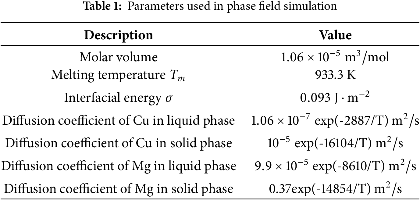
This paper establishes the KKS phase field model by using the regular solution method to define the free energy [22]. Each Gibbs free energy under multicomponent alloys is related to its associated thermodynamic factors, which can be described by a thermodynamic model as follows [23]:

G=G0+Gmixideal+GE(1)

Here, G0 represents the contribution from pure components, Gmixideal denotes the contribution from ideal mixing, and GE is the excess Gibbs free energy. For the Al-Cu-Mg ternary alloy, the Gibbs free energies of the solid phase GSreg and the liquid phase GLreg can be expressed as follows:

GSreg=∑i=13(ciSuiS0+RTciSIn⁡ciS)+GSex(2)

GLreg=∑i=13(ciLuiL0+RTciLIn⁡ciL)+GLex(3)

Here, S denotes the solid phase, L represents the liquid phase, subscript i refers to solute components 1 and 2, with i = 1 and i = 2, and i = 3 represents the solvent component; c is the solute concentration; uiS0 and uiL0 stand for the chemical formulas of the solid and liquid phases, respectively; R denotes the gas constant; T represents the thermodynamic temperature. The Gex values for the solid and liquid phases of the Al-Cu-Mg ternary alloy can be expressed as follows [23]:

GSex=C1C2[(−53520+2T)+(38590−2T)(C1−C2)+1170(C1−C2)2]+C1C3[(4971−3.5T)+(900+0.423T)(C1−C3)+950(C1−C3)2]+C2C3(−22279.28+5.868T)(4)

GLex=C1C2[(−66622+8.1T)+(46800−90.8T)(C1−C2)+10Tln⁡T(C1−C2)−2812(C1−C2)2]+C1C3[(−12000+8.566T)+(1894−3T)(C1−C3)+2000(C1−C3)2]+C2C3[(−36984+4.7561T)−8191.29(C2−C3)](5)

In the equation, C1, C2, and C3 represent the concentrations of Al, Cu, and Mg, respectively. The constants are sourced from fitting parameters in thermodynamic databases; for example, “−53520” and “38590” denote the interaction terms describing the Gibbs free energy between Al and Cu in the solid phase. These temperature-dependent terms are used to fit experimental data and accurately characterize the alloy’s thermodynamic behavior in the solid phase. In phase field models, the free energy density is typically coupled with thermodynamic databases, which can be specifically expressed as:

f(φ,c1,c2)=Wg(φ)+1vm{h(φ)Gsreg(c1,c2)+[1−h(φ)]Glreg(c1,c2)}(6)

In this equation, φ represents the phase field parameter, Vm denotes the molar volume, and the interpolation function h(φ) and double-well potential g(φ) can be expressed as follows:

h(φ)=φ3(10+6φ2−15φ)(7)

g(φ)=φ2(1−φ)2(8)

The solute composition at each position can be expressed as:

ci=h(φ)cis+(1−h(φ))cil       i=(1,2)(9)

When the two phases are in equilibrium, the chemical potentials of the solid and liquid phases are equal at any point, which can be expressed as:

uiL(ciL(x,t))=uiS(ciS(x,t))(10)

Thus, the phase field governing equation can be expressed as:

∂φ∂t=M(ε2∇2φ−fφ)(11)

fφ=h′(φ)[u1(c1S−c1L)+u2(c2S−c2L)+fS−fL]+Wg′(φ)(12)

∂ci∂t=∇{h(φ)∑j=1n−1DijS∇CjS+[1−h(φ)]∑j=1n−1DijL∇CjL}(13)

Here, DijS and DijL represent the solute diffusion coefficients in the solid and liquid phases, respectively, and M is the phase field mobility, which can be calculated by the following equation:

M-1=ε3σ2W(ℓ1(c1 Le,c1Se)D1+ℓ2(c2Le,c2 Se)D2)+ε2RT(1−Ke)βσVm(14)

ℓi=RT(ciLe,ciSe)2Vm∫01q(φ)dφ(15)

q(φ)=h(φ)[1−h(φ)][1−h(φ)]ciLe(1−ciLe)+h(φ)ci Se(1−ciSe)φ(1−φ)(16)

Here, ciLe and ciSe represent the concentration distribution of solute components in equilibrium, Ke denotes the partition coefficient, Vm is the molar volume, me is the slope of the liquidus, and cSe=KecLe represents equilibrium. D1 and D2 are the diffusion coefficients of two different solutes, β is the dynamic coefficient, and σ represents interfacial energy. Anisotropy is introduced into the phase field model via the interfacial energy-related parameter ε.

ε(θi)=ε0(1+vcos⁡(kθi))(17)

ε0=6λθ2.2(18)

Here, θ represents the angle between the x-axis and the preferred growth direction of the grain, with subscript i denoting a specific grain and k representing the symmetry coefficient, which is set to 4 in this study’s phase field model calculations. v denotes the anisotropy intensity coefficient. By combining the phase field equation with the solute field equation, the model is established, and the solute field equation can be expressed as:

∂ci∂t=∇(Di(φ)fcici∇fci)       i=(1,2)(19)

Here, fci and fcici represent the first and second derivatives of free energy with respect to concentration, respectively.

2.2 Machine Learning Model

2.2.1 BP Neural Network

The fundamental idea of the BP neural network is to adjust the network’s weights and biases to make the output as close as possible to the target value [24]. Its core lies in the error backpropagation algorithm, which calculates the gradient of the error with respect to each weight using the chain rule and optimizes using gradient descent. The network structure includes an input layer, hidden layers, and an output layer. The input layer primarily receives external signals, and the hidden layer(s) are between the input and output layers; there may be one or more hidden layers, each composed of several neurons that use activation functions for nonlinear transformation of input signals, while the output layer produces the network’s final prediction. The training process of the BP neural network follows these steps:

(1) The input data is transmitted through the input layer to the hidden layer, where it undergoes a nonlinear transformation via the activation function before passing to the next layer, until reaching the output layer.

(2) The gradient of the error at the output layer is calculated and propagated backward layer by layer using the chain rule, determining the error gradient for each hidden layer.

(3) Update the weights and biases: Based on gradient descent, the weights and biases in the network are adjusted to gradually reduce the error. The update formula is as follows:

wij(t+1)=wij(t)−η∂E∂wij(t)(20)

bi(t+1)=bi(t)−η∂E∂bi(t)(21)

Here, wij(t) denotes the weight at the t-th iteration, bi(t) is the bias at the t-th iteration, η represents the learning rate, and E is the loss function.

(4) Repeat the above process until the error converges to a predefined threshold or the maximum number of iterations is reached.

2.2.2 Grey Wolf Optimization Algorithm

The GWO simulates the natural leadership hierarchy and cooperative hunting behavior of wolves by defining four distinct roles to represent the social structure within the pack. The optimal solution corresponds to the Alpha wolf (α), which leads the entire group. The second- and third-best solutions are designated as the Beta wolf (β) and Delta wolf (δ), respectively, assisting the Alpha wolf during the hunt. All other candidate solutions are classified as Omega wolves (ω), which follow the guidance of the α, β, and δ wolves. This role-based hierarchy models the wolves’ social structure mathematically, enabling the algorithm to effectively balance exploration and exploitation within the search space. Optimization proceeds by simulating behaviors such as encircling, tracking, and attacking prey. During the hunting process, the wolf pack first encircles the prey, which can be mathematically described as follows [25]:

D→=|C→⋅Xp→(t)−X→(t)|(22)

X→(t+1)=Xp→(t)−A→⋅D→(23)

Eq. (22) represents the distance between an individual and the prey during iterations, while Eq. (23) is the position update formula for the wolves in each iteration, with t representing the current iteration count. A→ and C→ are coefficient vectors, where Xp→ and X→ represent the position vectors of the prey and the wolves, respectively. The formulas for calculating A→ and C→ are as follows:

A→=2α→⋅r1→−α→(24)

C→=2⋅r2→(25)

Here, r1→ and r2→ are random number vectors, and α→ is the convergence factor, which decreases linearly with each iteration.

α→=2(1−tT)(26)

Here, t represents the current iteration count, and T stands for the maximum iterations allowed.

Grey wolves can locate the prey’s position and proceed to encircle it. Once they lock onto the prey, β and γ, under the guidance of α, direct the pack to encircle the prey. The mathematical model describing how individual wolves track the prey’s position is as follows:

{Dα→=|C1→⋅Xα→−X→|Dβ→=|C2→⋅Xβ→−X→|Dδ→=|C3→⋅Xδ→−X→|(27)

Here, Dα→, Dβ→ and Dδ→ respectively represent the distances between α, β and δ and other individuals; Xα→, Xβ→ and Xδ→ respectively denote the current positions of α, β and δ; C1→, C2→ and C3→ are random vectors, and X→ is the current position of the grey wolf.

{X1→=Xα→−A1→⋅Dα→X2→=Xβ→−A2→⋅Dβ→X3→=Xδ→−A3→⋅Dδ→(28)

X→(t+1)=X1→+X2→+X3→3(29)

Eq. (28) defines the step size and direction of the ω individual in the wolf pack as it moves toward α, β, and δ, while Eq. (29) defines the final position of ω. When the prey stops moving, the grey wolves attack to complete the hunting process. The iterations are repeated and updated until either the maximum number of iterations is reached or the convergence criteria are met.

2.2.3 LSGWO-BP Model

Chaotic mapping algorithms play a critical role in the improvement of intelligent optimization algorithms. This experiment thoroughly considers the convenience of enhancing intelligent optimization algorithms, and comprehensively compares three improved mappings: Circle-Root mapping, Tent-Cosine mapping, and Logistic-Sine mapping.

(1) Circle-Root mapping: This mapping combines Circle mapping with the square root function. First, the input position undergoes a linear transformation to reduce its scale by a certain proportion, followed by a nonlinear mapping using Circle mapping, and finally, the result is further adjusted with the square root function. This combination generates more complex dynamic behaviors, facilitating the exploration of different parameter spaces.

(2) Tent-Cosine mapping: This mapping combines the Tent mapping and the cosine function. First, the Tent mapping performs a piecewise linear mapping on the input position, followed by nonlinear adjustment with the cosine function. This combination enhances the algorithm’s robustness to data variations or noise, making it more reliable and stable in applications.

(3) Logistic-Sine mapping: This mapping integrates the properties of the Logistic nonlinear mapping and the sine function, capable of producing various chaotic behaviors. By adjusting parameters, the system can gradually transition from a stable state to a chaotic state, thereby achieving effective control over dynamic behavior.

Fig. 1 presents the convergence curve and optimal fitness values observed during the grey wolf optimization process. Compared to the Circle-Root and Tent-Cosine mappings, the Logistic-Sine mapping achieves faster convergence toward the global optimum, reaching a more accurate final result within approximately 32 iterations. Specifically, the Logistic-Sine mapping attains an optimal fitness value of 0.270821, which slightly surpasses the Circle-Root mapping’s 0.27089 and the Tent-Cosine mapping’s 0.2709, demonstrating its superior search precision and convergence speed in enhancing the grey wolf algorithm. This improved performance stems from the Logistic-Sine mapping’s effective combination of the chaotic dynamics inherent in the Logistic mapping and the periodic properties of the Sine mapping, thereby making the search process both more efficient and precise. Consequently, this study adopts the Logistic-Sine mapping to further refine the grey wolf algorithm for optimizing the BP neural network.

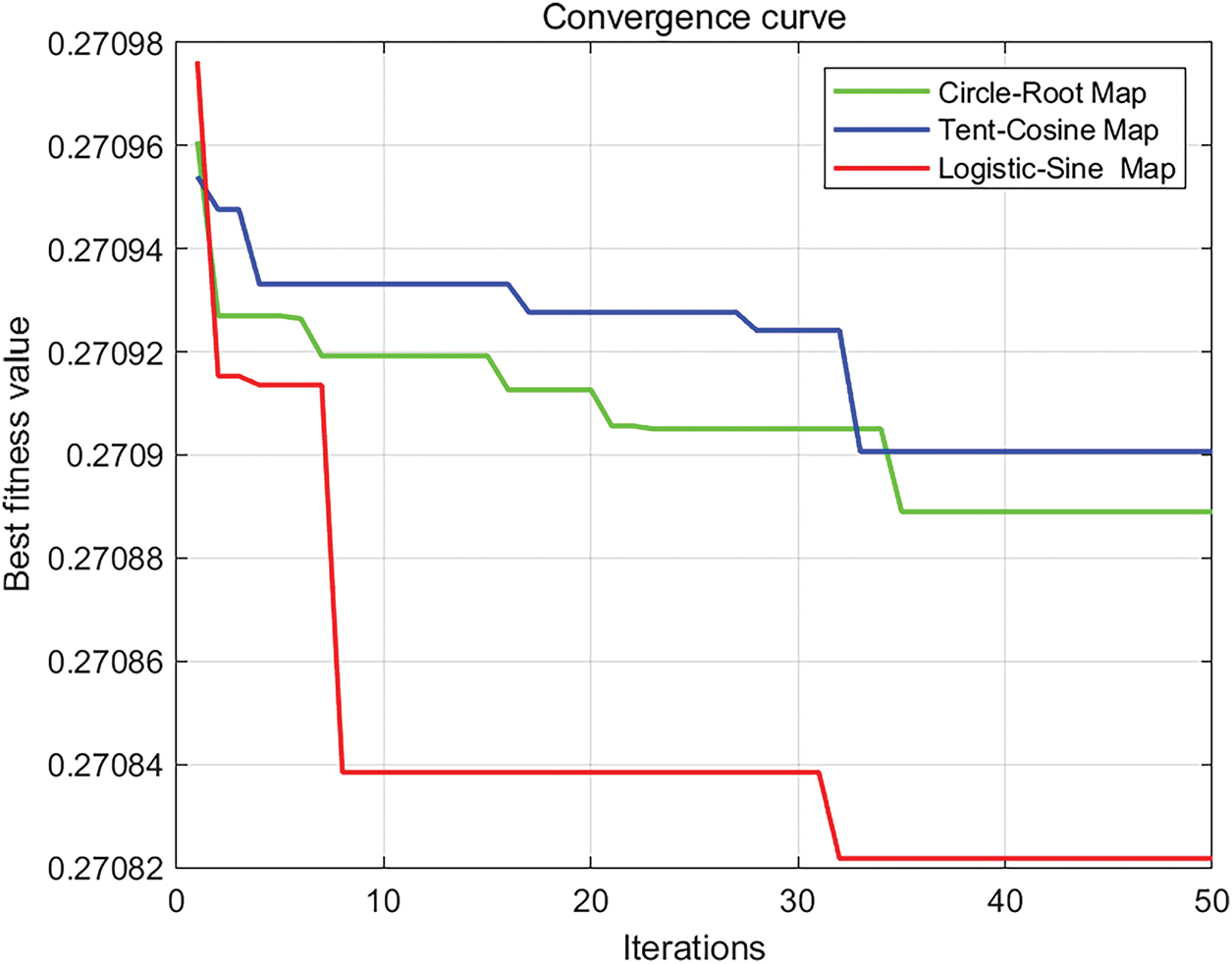
Figure 1: Convergence curves of three improved mappings

This study initializes the GWO population using Logistic-Sine mapping, integrating grey wolf group behavior characteristics and chaotic mapping techniques to increase population diversity, enhance global and local search abilities, and avoid local optimal solutions. The algorithm uses Logistic-Sine mapping to generate chaotic sequences to update the positions of wolves. Then, the fitness value corresponding to each wolf’s position is calculated, updating the positions of α, β, and δ wolves according to the fitness values. Finally, the positions of other wolves are updated based on the leaders’ positions, repeating the steps until reaching the maximum iterations or satisfying convergence conditions. Fig. 2 compares the bifurcation behavior of the Logistic-Sine map and the traditional Logistic map under different chaos control parameters r, clearly illustrating the differences in their chaotic dynamic characteristics. The results indicate that, after entering the chaotic regime, the conventional Logistic map still exhibits pronounced periodic windows, whereas the Logistic-Sine map, by introducing a nonlinear sine perturbation, effectively attenuates these windows’ prominence, yielding a more continuous and uniformly distributed chaotic region.

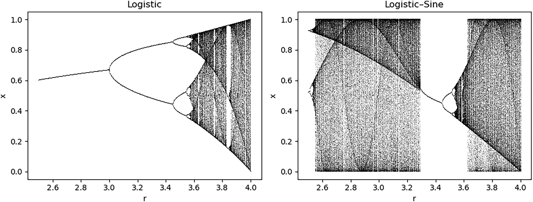
Figure 2: Comparison of bifurcation diagrams between the Logistic-Sine map and the Logistic map

The Logistic-Sine mapping generates chaotic sequences by the following formula [26]:

xit+1=sin⁡(π⋅(4⋅xit⋅(1−xit)))(30)

Here, xit is the value at the i-th position in the t-th iteration, and xit+1 is the updated value at the i-th position in the (t + 1)-th iteration after applying the Logistic-Sine mapping, 4 is the chaos control parameter. This formula generates a chaotic sequence, which is then mapped to the upper and lower limits of the search space to determine the initial population’s positions. The specific steps of optimizing the BP neural network using the LSGWO algorithm are as follows:

(1) Design an appropriate BP neural network structure based on the characteristics of the regression prediction problem, and initialize the network’s weights and biases.

(2) Use the weights and biases of the BP neural network as optimization variables, and optimize them with the LSGWO algorithm.

(3) Train and optimize the BP neural network using the optimized weights and biases, continuously adjusting the network parameters with the backpropagation algorithm to reduce prediction error.

(4) Use the trained LSGWO-BP neural network model to predict the test data and evaluate the accuracy and performance of the prediction results.

By combining the LSGWO algorithm with the BP neural network, the global search capability of the LSGWO algorithm and the nonlinear modeling ability of the BP neural network can be fully utilized to improve the accuracy and stability of regression predictions. Fig. 3 shows the process framework of the Logistic-Sine mapping improved grey wolf optimization BP neural network:

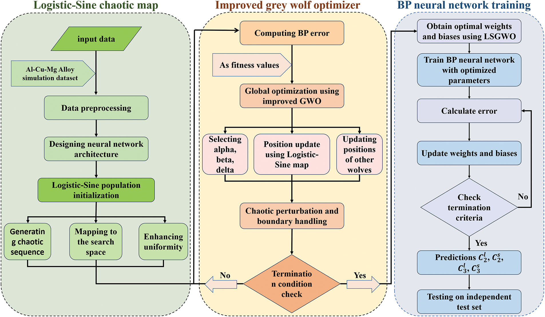
Figure 3: Framework diagram of Logistic-Sine mapping improved grey wolf optimized BP neural network

3  Experimental Results

3.1 Experimental Setup

Based on the Al-Cu-Mg ternary alloy, this work establishes a KKS phase field model and depicts the growth process in its equilibrium phase diagram via Fig. 4. In this process, the primary S phase nucleates within the liquid phase and gradually grows, undergoing an L→S phase transformation as the temperature decreases, as indicated by the red circle in Fig. 4a. Upon additional cooling, the crystal nuclei continuously enlarge (as shown in Fig. 4b), and several dendrites compete for growth, forming various shapes as a result of their interactions. Fig. 4c presents the numerical simulation results of simultaneous growth of multiple grains within the solute field distribution. The specific physical parameters required for the experimental process are provided in Table 1.

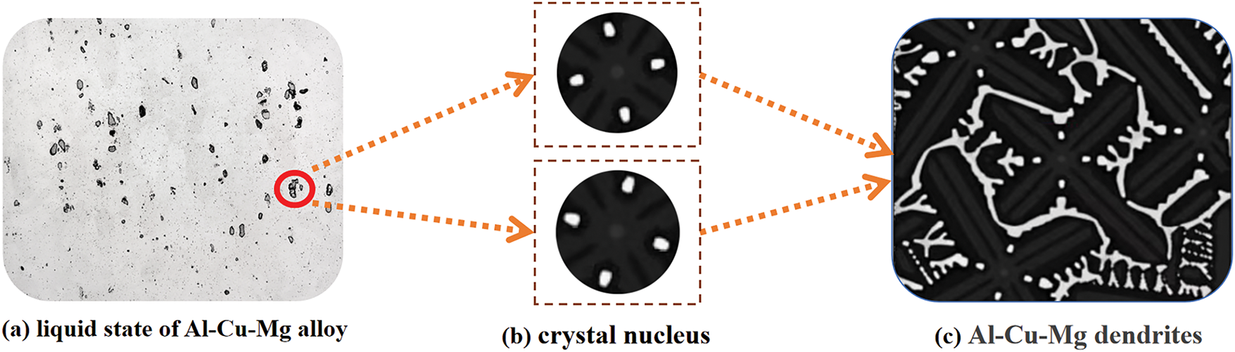
Figure 4: Schematic diagram of the growth process of the Al-Cu-Mg ternary alloy

The LSGWO-BP algorithm was constructed and compared with six other machine learning models, including the traditional backpropagation neural network (BP), Extremely Randomized Trees (ET), Random Forest (RF), AdaBoost, Linear Regression (LR), and Decision Tree (DT). ET is an ensemble learning method for classification and regression that generates decision trees by incorporating additional randomness into the splitting process, thereby enhancing the model’s predictive accuracy and generalization performance [27]. As a variant of decision tree ensembles, ET is similar to RF but introduces greater randomization during tree construction to reduce variance. RF is a widely adopted ensemble learning algorithm known for its robustness in classification and regression tasks. It constructs multiple decision trees and aggregates their outputs to make final predictions, thereby improving model stability and reducing overfitting [28]. AdaBoost is another ensemble technique designed to improve classification accuracy by sequentially training a series of weak classifiers, where each subsequent model focuses on correcting the errors of its predecessor [29]. The core principle of AdaBoost is to increase the weights of previously misclassified samples, allowing the model to focus more on difficult cases and incrementally enhance overall accuracy. LR is a statistical learning method used to model the linear relationship between independent variables (features) and a dependent variable (target). Despite its simplicity, LR remains a powerful and widely used regression technique for predicting continuous outcomes [30]. DT constructs a predictive model by recursively partitioning the dataset based on feature values, forming a tree structure in which internal nodes represent attribute tests and leaf nodes correspond to output values or categories. The recursive splitting continues until a predefined stopping criterion is met or the data in each subset becomes homogeneous [31].

This paper uses 490,000 data samples as the basis for the experiments. To ensure the fairness and comparability of the experiment, we used a common method of dividing the data set into training, testing, and validation sets in an 8:1:1 ratio. The training set is used for model training and parameter adjustment, the test set for evaluating the model’s generalization ability, and the validation set for monitoring model performance and adjusting hyperparameters during training. During the preparation of the training data, phase-field model parameters C2, C3, and φ were used as input independent variables, while the metallic species Cu and Mg under various states (indices C2l, C2s, C3l, and C3s) served as output dependent variables. This setup reflects the physical linkage between inputs and outputs grounded in the KKS phase-field model’s thermodynamic equilibrium and dynamics: input parameters govern solute partitioning between solid and liquid via the free-energy functional and concentration-weighted constraints, and the machine learning model learns this mapping in a data-driven manner.

Considering that the regression task in this study involves mapping 3 input dimensions to 4 output dimensions, characterized by a low-dimensional input space and sufficient sample size, to avoid empirical biases in network architecture design and improve model performance, this work introduces neural architecture search (NAS) to optimize the number of neurons in the hidden layer. As shown in Fig. 5, during the search process, the average mean squared error (MSE) on the validation set was used as the evaluation metric. Through comparative analysis of multiple structural configurations, it was determined that setting 9 neurons in the hidden layer yielded the optimal predictive performance. Therefore, a three-layer network structure of 3–9–4 was adopted as the fundamental framework for the regression model. To prevent overfitting during training, the MSE on the validation set was monitored in real time, and an early stopping mechanism was introduced: training was terminated immediately if the validation set MSE did not significantly decrease over several consecutive epochs. This strategy ensures adequate model training while effectively enhancing its generalization capability. The MSE calculation method is as follows: the squared errors for all validation samples across the 4 output dimensions are computed separately, then averaged overall to comprehensively assess the prediction accuracy across the entire output space.

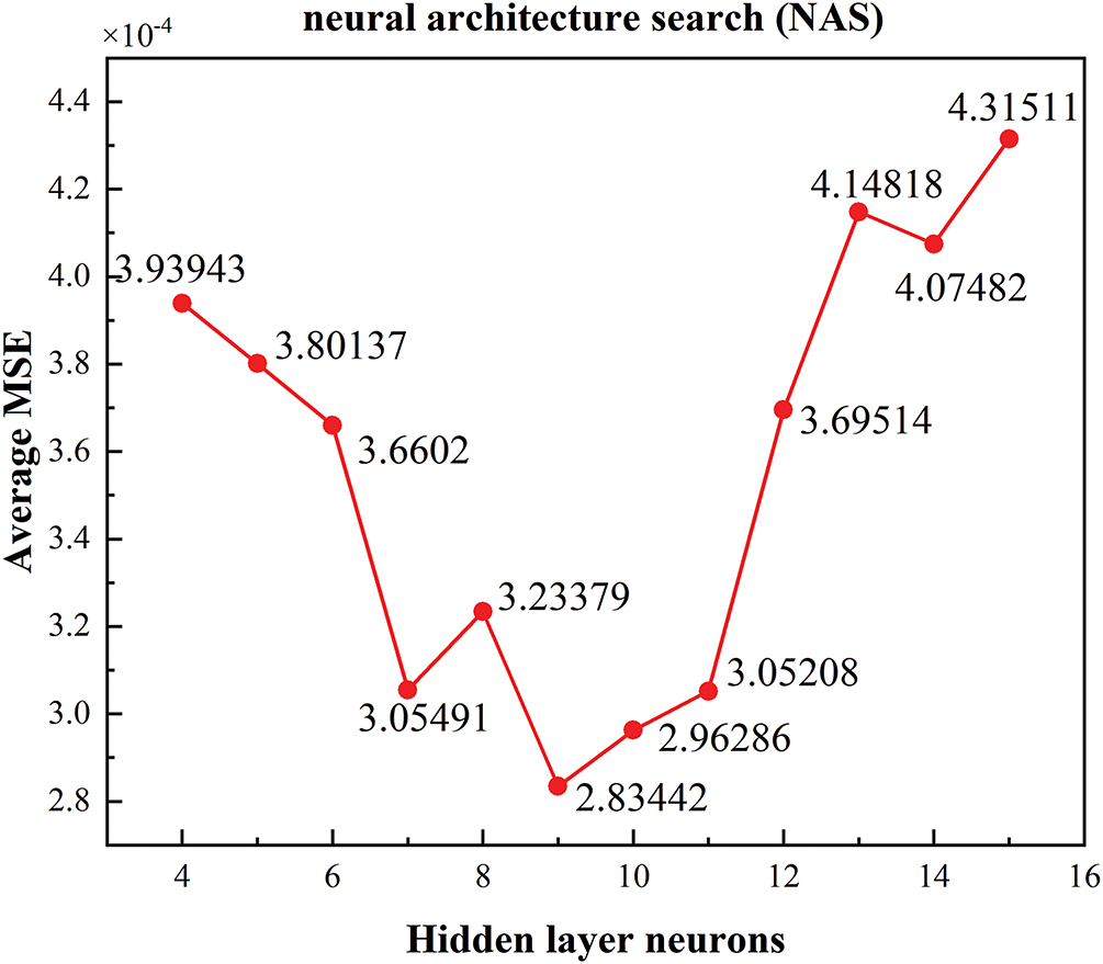
Figure 5: Comparison of average MSE under different numbers of hidden layer neurons

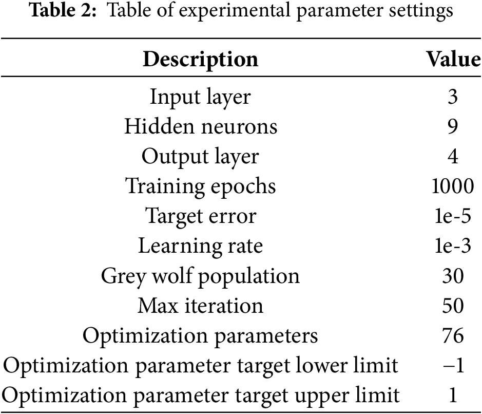
To ensure adequate training, the number of training epochs was ultimately set to 1000, with a learning rate of 1e-3 and a target error of 1e-5. When using the LSGWO algorithm to optimize the neural network weights and biases, we set the grey wolf population size to 30 and the maximum number of iterations to 50. According to the network structure, the total number of optimized parameters is 76, including 27 weights from the input layer to the hidden layer, 36 weights from the hidden layer to the output layer, 9 biases for the hidden layer, and 4 biases for the output layer, with parameter values ranging within [−1, 1]. Specifically, all parameter lower limits were set to −1 and upper limits to 1 to ensure parameter variation within a reasonable range, preventing overly large or small parameter values from impacting model stability and performance. The hidden layer of the feedforward neural network uses the hyperbolic tangent function tansig as the activation function, and the output layer uses the activation function purelin. Table 2 presents the specific experimental parameter settings.

In this study, the LSGWO-BP model required approximately 4–6 min per training session on a computing platform equipped with an Intel Core i7-12700H CPU, with peak memory usage around 2 GB and no need for a dedicated GPU. In contrast, traditional phase-field quasi-equilibrium numerical simulations (with an 800 × 800 grid) required several hours for a single solution under the same hardware environment, with memory usage often exceeding 10 GB. Furthermore, after training, the LSGWO-BP model achieved a single prediction time of approximately 0.2 ms, representing a significant speed improvement. Efficiency comparisons clearly demonstrate that the introduction of the LSGWO-BP method not only significantly accelerates subsequent large-scale high-throughput simulation processes but also completes model optimization and validation within an acceptable computational resource budget. To systematically present the overall framework and logical structure of this study, a mind map was constructed, as shown in Fig. 6.

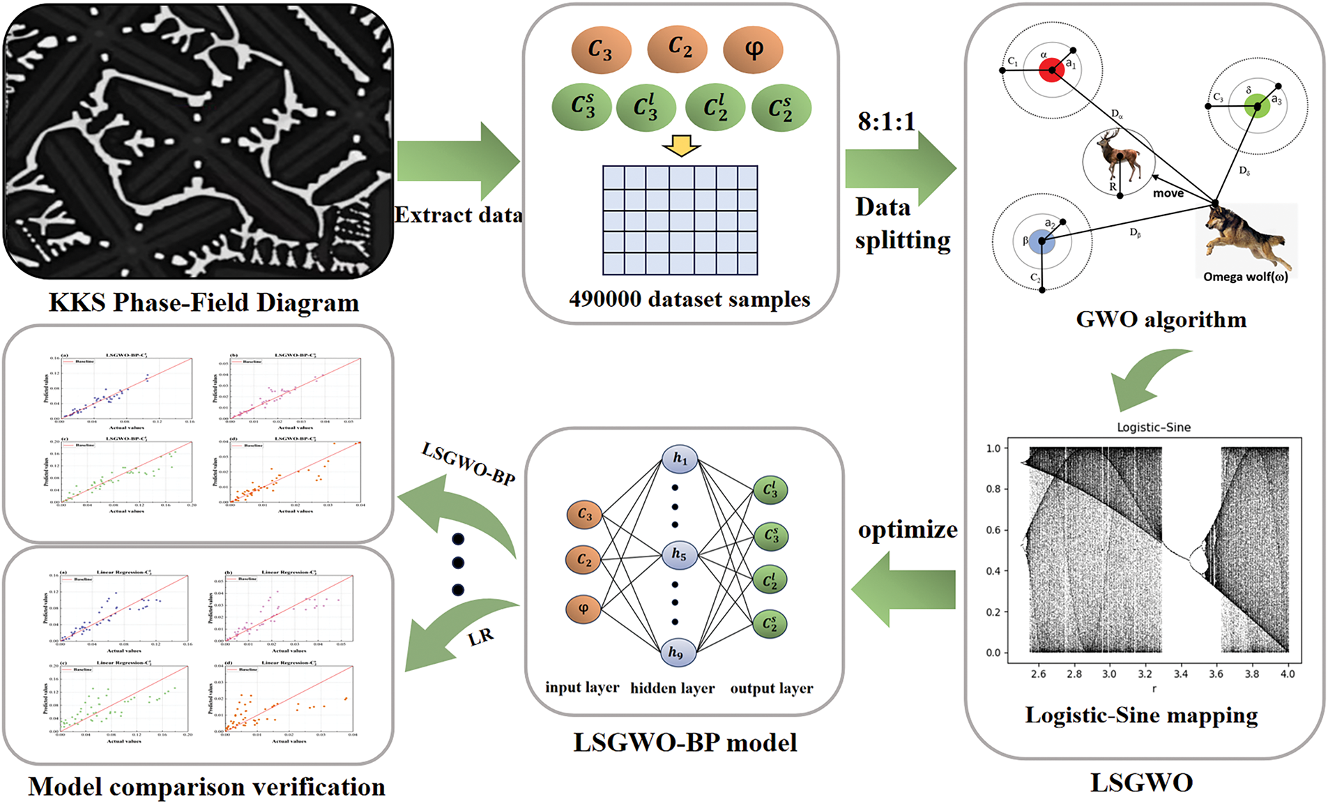
Figure 6: Technical roadmap for quasi-phase equilibrium prediction in the KKS phase-field model based on the LSGWO-BP method

3.2 Testing of the LSGWO Algorithm

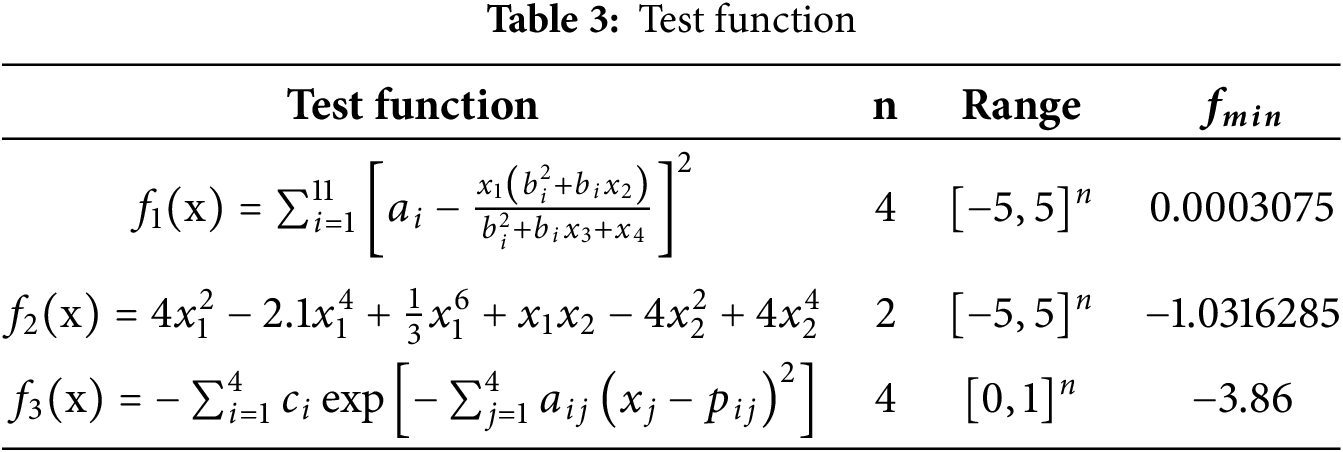
The model developed in this study adopts a multi-input multi-output structure, where the output variables correspond to different physical quantities of the liquid and solid phases. However, due to the strong physical coupling among the output variables and their highly similar numerical ranges and trends, these outputs exhibit weak distinguishability during optimization. Based on these characteristics, the problem can be simplified to a multi-input single-output formulation to facilitate algorithm performance analysis and evaluation. Therefore, three representative types of standard benchmark functions were selected in this study, as shown in Table 3. These functions are widely used in evaluating optimization algorithm performance, covering various dimensions, domains, and global optimum characteristics. These benchmarks facilitate a comprehensive assessment of the proposed algorithm from multiple perspectives, including search capability, convergence speed, and robustness.

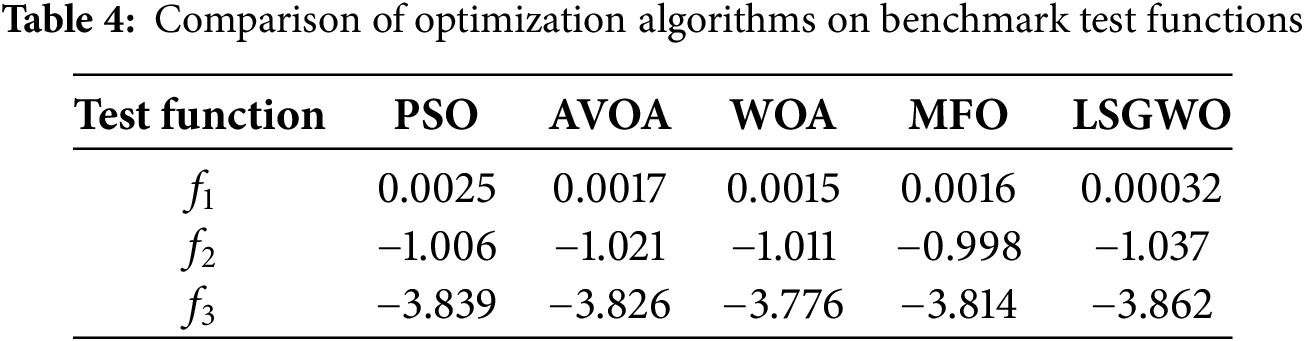
To further validate the adaptability and solving capability of the proposed optimization algorithm, four representative classical optimization algorithms were selected for comparison experiments: Particle Swarm Optimization (PSO) [32], African Vulture Optimization Algorithm (AVOA) [33], Whale Optimization Algorithm (WOA) [34], and Moth-Flame Optimization (MFO) [35]. Fig. 7 illustrates the 3D search spaces and fitness evolution curves of the selected test functions, while Table 4 presents the performance comparison of the algorithms across different test functions. As shown in Fig. 7 and Table 4, the proposed LSGWO optimization algorithm consistently outperforms the others across all three types of benchmark functions.

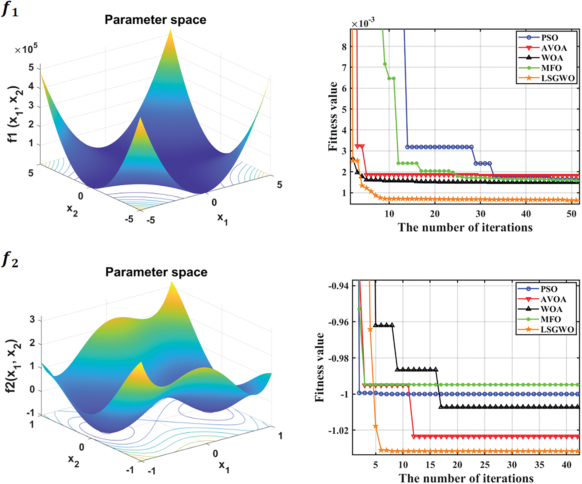
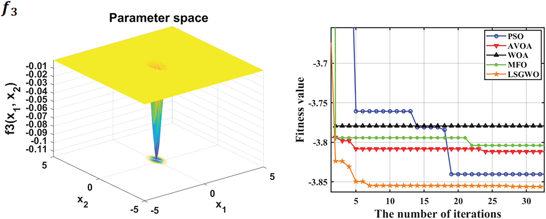
Figure 7: 3D plots and fitness convergence curves of benchmark test functions

3.3 Evaluation Metrics

This study establishes a quasi-equilibrium regression prediction for the phase-field model and evaluates the predictive performance of the training model using five metrics: Mean Absolute Error (MAE), Mean Squared Error (MSE), Root Mean Square Error (RMSE), Mean Absolute Percentage Error (MAPE), and the Coefficient of Determination (R2). The formulas for each evaluation metric are as follows:

MAE(y,y∧)=1n∑i=1n|(yi−yi∧)|(31)

MSE(y,y∧)=1n∑i=1n(yi−yi∧)2(32)

RMSE(y,y∧)=1n∑i=1n(yi−yi∧)2(33)

MAPE(y,y∧)=1n∑i=1n(|yi−yi∧|yi)(34)

R2(y,y∧)=1−∑i=1n(yi∧−yi)2∑i=1n(yi−−yi)2(35)

In model evaluation, yi represents the true values, yi∧ represents the predicted values obtained from the Logistic-Sine mapped Grey Wolf Optimized BP Neural Network model and six machine learning models, and yi− is the mean observed value of the samples. MSE is used to measure the mean squared difference between the predicted and actual values, while RMSE, as the square root of MSE, provides information on the standard deviation of prediction errors. MAE calculates the mean absolute difference between the predicted and actual values. R2 evaluates the model’s ability to explain the variance in the data; the closer its value is to 1, the better the model fits the data. MAPE provides the mean percentage error of the predicted values relative to the true values; the smaller the value, the higher the prediction accuracy. Collectively, these evaluation metrics offer a comprehensive basis for evaluating the predictive performance of the model.

3.4 Model Evaluation Result Analysis

Figs. 8–19 show the performance of the LSGWO-optimized BP neural network and six commonly used machine learning models across multiple training datasets. As shown in Table 5, the LSGWO-BP model demonstrates outstanding performance across all datasets based on comparisons of the MAE, MSE, RMSE, MAPE and R2 evaluation metrics.

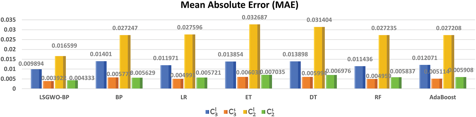
Figure 8: Comparison of MAE results

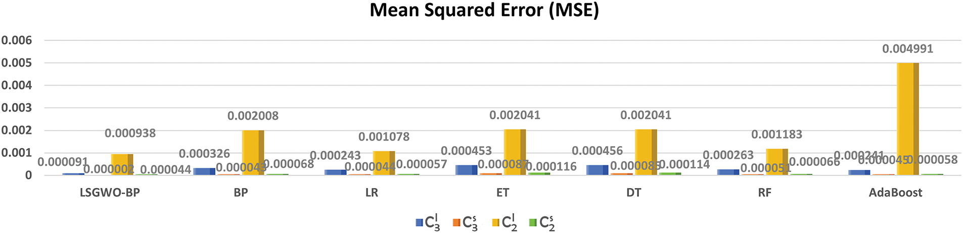
Figure 9: Comparison of MSE results

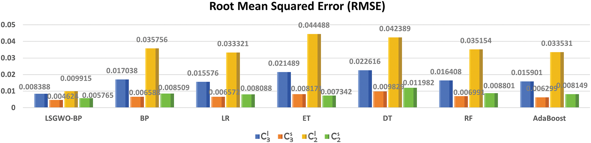
Figure 10: Comparison of RMSE results

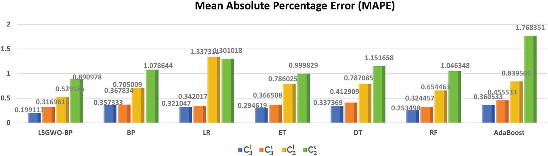
Figure 11: Comparison of MAPE results

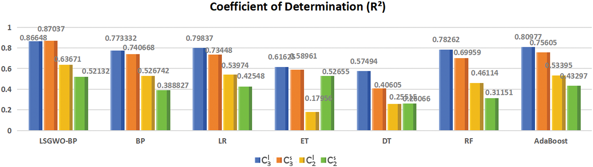
Figure 12: Comparison of R2 results

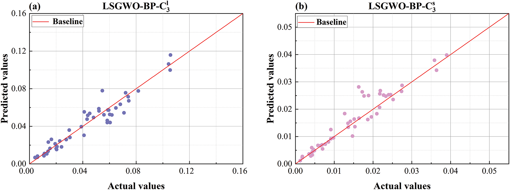
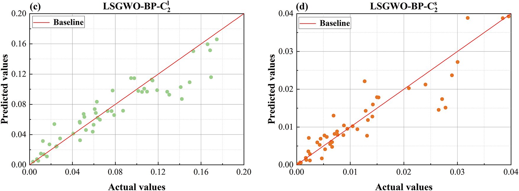
Figure 13: Comparison plot of LSGWO-BP predicted values and actual values (a) predicted vs. actual values comparison plot for C3l (b) predicted vs. actual values comparison plot for C3s (c) predicted vs. actual values comparison plot for C2l (d) predicted vs. actual values comparison plot for C2s

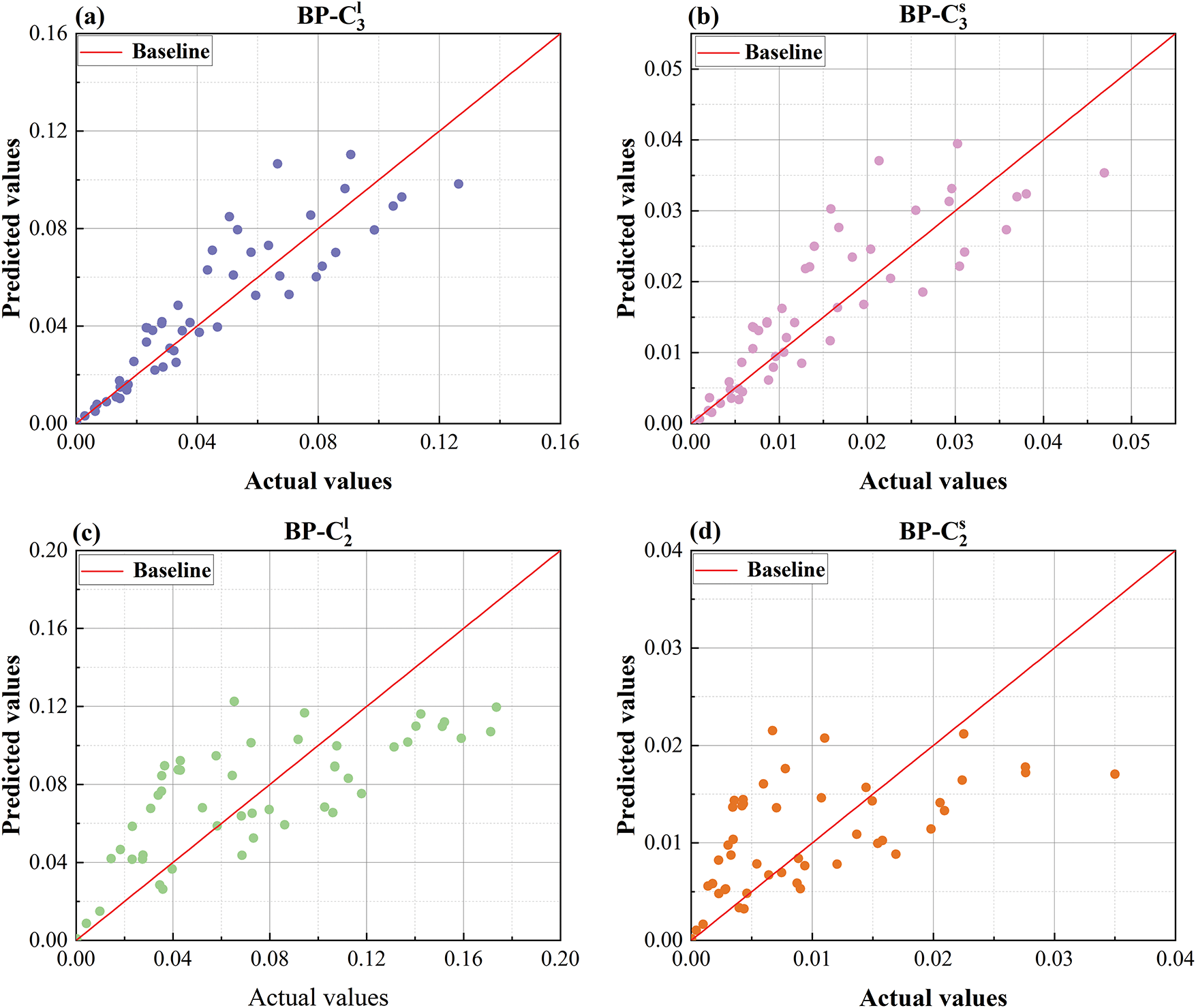
Figure 14: Comparison plot of BP predicted values and actual values (a) predicted vs. actual values comparison plot for C3l (b) predicted vs. actual values comparison plot for C3s (c) predicted vs. actual values comparison plot for C2l (d) predicted vs. actual values comparison plot for C2s

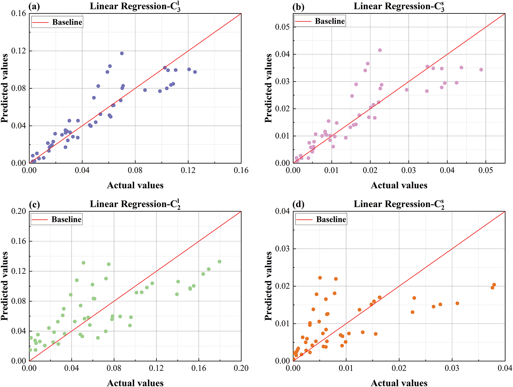
Figure 15: Comparison plot of LR predicted values and actual values (a) predicted vs. actual values comparison plot for C3l (b) predicted vs. actual values comparison plot for C3s (c) predicted vs. actual values comparison plot for C2l (d) predicted vs. actual values comparison plot for C2s

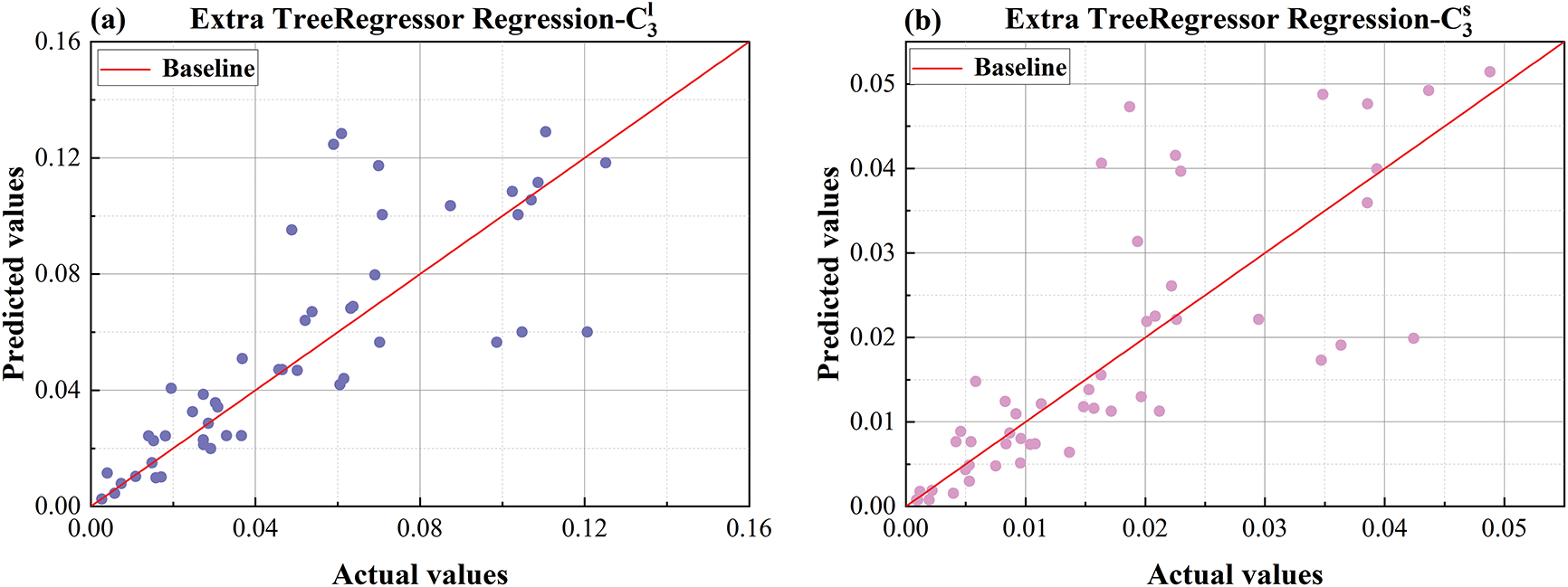
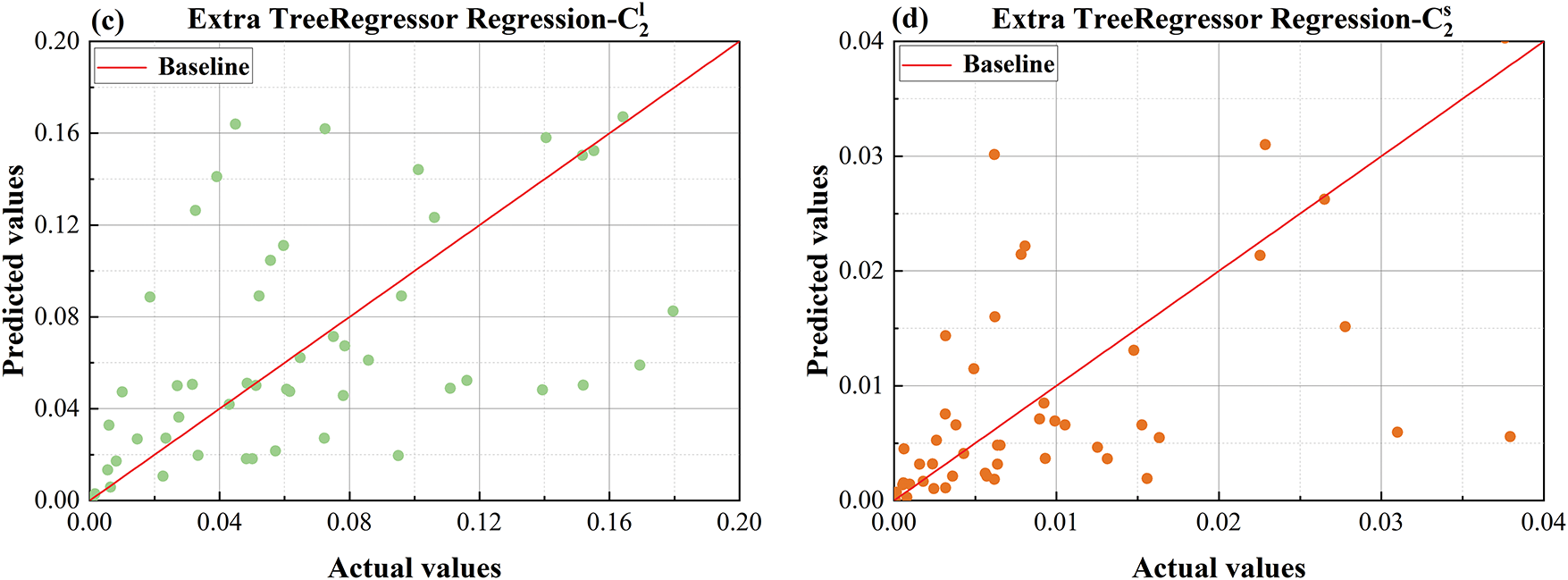
Figure 16: Comparison plot of ET predicted values and actual values (a) predicted vs. actual values comparison plot for C3l (b) predicted vs. actual values comparison plot for C3s (c) predicted vs. actual values comparison plot for C2l (d) predicted vs. actual values comparison plot for C2s

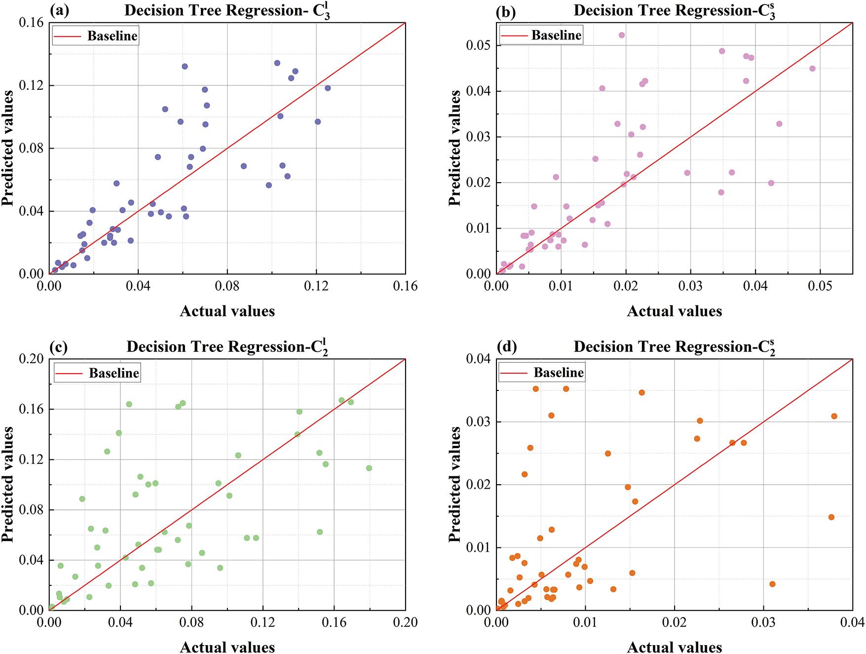
Figure 17: Comparison plot of DT predicted values and actual values (a) predicted vs. actual values comparison plot for C3l (b) predicted vs. actual values comparison plot for C3s (c) predicted vs. actual values comparison plot for C2l (d) predicted vs. actual values comparison plot for C2s

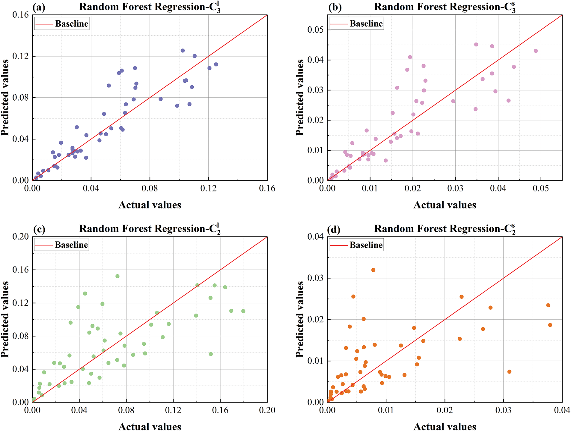
Figure 18: Comparison plot of RF predicted values and actual values (a) predicted vs. actual values comparison plot for C3l (b) predicted vs. actual values comparison plot for C3s (c) predicted vs. actual values comparison plot for C2l (d) predicted vs. actual values comparison plot for C2s

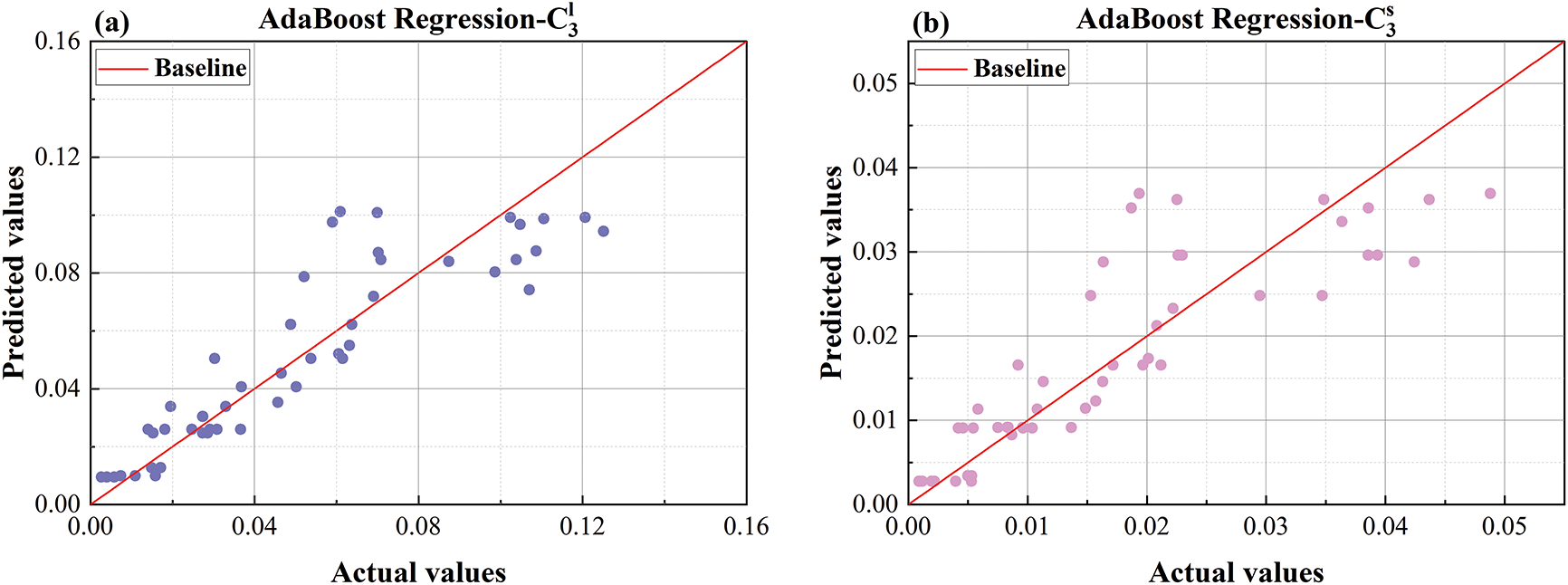
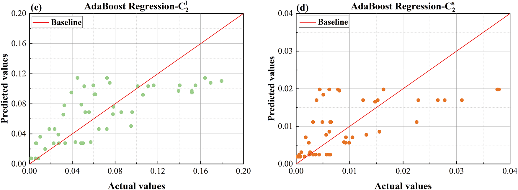
Figure 19: Comparison plot of AdaBoost predicted values and actual values (a) predicted vs. actual values comparison plot for C3l (b) predicted vs. actual values comparison plot for C3s (c) predicted vs. actual values comparison plot for C2l (d) predicted vs. actual values comparison plot for C2s

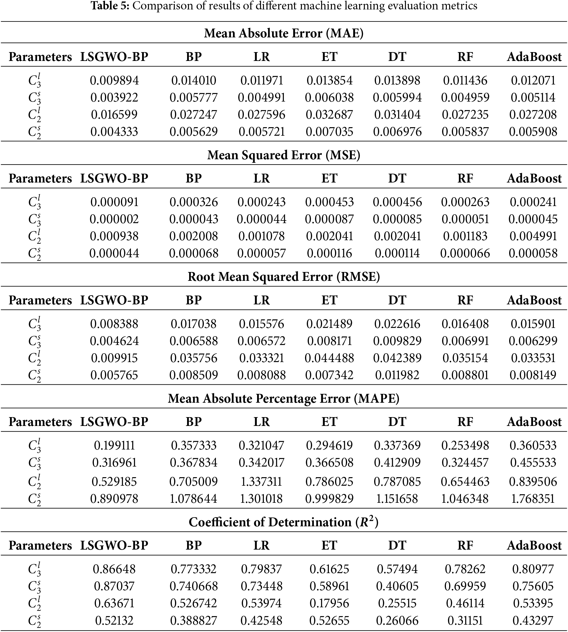
Fig. 8 presents a bar chart comparing the MAE results of different models. The LSGWO-BP model consistently achieves lower MAE values than the six baseline machine learning models across all four prediction outputs, indicating superior predictive accuracy. For C3l, the RF model yields the best performance among the six traditional models with an MAE of 0.011436, whereas the LSGWO-BP model achieves a lower MAE of 0.009894. For C3s, RF again performs best among the baseline models with an MAE of 0.004959, while LSGWO-BP further reduces the error to 0.003922. Regarding C2l, AdaBoost produces the best result among the six models, with an MAE of 0.027208, while LSGWO-BP achieves a lower value of 0.016599. For C2s, BP performs best among the baseline models with an MAE of 0.005629, compared to 0.004333 for LSGWO-BP.

Fig. 9 presents a bar chart comparing the MSE values for different models. For C3l, AdaBoost achieves the best performance among the six conventional machine learning models with an MSE of 0.000241, whereas the LSGWO-BP model yields a substantially lower MSE of 0.000091. For C3s, BP attains the best result among the baseline models with an MSE of 0.000043, while LSGWO-BP achieves an even lower error of 0.000002. For C2l, LR again provides the best performance among the six models with an MSE of 0.001078, while LSGWO-BP reduces the error to 0.000938. In the case of C2s, LR obtains the lowest MSE among the traditional models at 0.000057, but the LSGWO-BP model achieves a better result of 0.000044. Overall, Fig. 9 clearly demonstrates that the LSGWO-BP model consistently outperforms the traditional machine learning models in terms of predictive accuracy based on MSE.

Fig. 10 presents a bar chart comparing the RMSE results across different models. For C3l and C2l, the LR model achieves the best performance among the six baseline machine learning models, with RMSE values of 0.015576 and 0.033321, respectively. In comparison, the LSGWO-BP model attains lower RMSE values of 0.008388 for C3l and 0.009915 for C2l. For C3s and C2s, AdaBoost and ET provide the best results among the traditional models, with RMSE values of 0.006299 and 0.007342, respectively. The LSGWO-BP model, however, further reduces these errors to 0.004624 and 0.005765. Overall, Fig. 10 demonstrates that the LSGWO-BP model exhibits the lowest overall fluctuation in prediction error, indicating greater stability and consistency across different prediction tasks.

Fig. 11 shows the MAPE comparison histogram, where LSGWO-BP also performs exceptionally well in terms of MAPE. For C3l, C3s, and C2l, RF yielded the optimal results among six machine learning methods, with MAPE values of 0.253498, 0.324457, and 0.654463, respectively, while LSGWO-BP’s MAPE values were 0.199111, 0.316961, and 0.529185. For C2s, the best traditional machine learning model was ET, with a MAPE value of 0.999829, which is notably higher than that of LSGWO-BP, at 0.890978. It is evident that LSGWO-BP exhibits the smallest relative errors across the four prediction datasets, showcasing its superiority in error management.

Fig. 12 is a histogram comparing R2 results, where the minimum value of LSGWO-BP across the four datasets exceeds 0.52. For C3l and C3s, the optimal traditional machine learning model is AdaBoost, with R2 values of 0.80977 and 0.75605, respectively, while LSGWO-BP achieves R2 values of 0.86648 and 0.87037. For C2l and C2s, the best traditional machine learning models were LR and ET, with R2 values of only 0.53974 and 0.52655, whereas LSGWO-BP achieved R2 values of 0.63671 and 0.52132, respectively. Although LSGWO-BP does not exhibit a distinct advantage for C2s, its overall performance in R2 values across the four datasets is still superior.

To present a more intuitive comparison of model predictive performance, Figs. 13–19 show comparison plots of predicted and actual values for each dataset. Given the large volume of data, a random subset of 50 samples from each dataset was selected for visualization. As shown in Fig. 13, the LSGWO-BP model produces predicted values that align more closely with the actual values than those generated by the six baseline machine learning models, indicating superior fitting accuracy. In contrast, the traditional models exhibit larger prediction deviations, particularly in the C2l and C2s datasets, where their fitting curves appear less consistent with the true values. These results further highlight the strong predictive capability of the LSGWO-BP model in complex data scenarios–maintaining its advantage even under sample reduction conditions.

As shown in the regression scatter plots in Fig. 14, the traditional BP exhibits certain performance limitations in predicting multicomponent alloy KKS phase-field models. The main reason lies in the fact that BP neural networks rely on gradient descent for parameter updates, which makes them prone to local optima and sensitive to initial weights, thereby limiting their generalization capability. When dealing with highly nonlinear and complexly coupled microstructural evolution data in materials, traditional BP models struggle to comprehensively capture the global features in the parameter space. As a result, its prediction accuracy and stability are significantly inferior to those of the LSGWO-BP model.

As shown in Fig. 15, which compares the predicted and actual values using the LR model, LR exhibits relatively poor predictive accuracy for the C2l and C2s datasets. This limitation likely stems from the inherently linear nature of the LR model, which hampers its ability to capture complex nonlinear relationships and makes it sensitive to variations in feature diversity. As a result, LR struggles to represent intricate data patterns and interaction effects in highly nonlinear regions, leading to noticeable discrepancies between its predictions and the true values.

From Fig. 16, which shows the comparison plot of ET predicted vs. actual values, it can be seen that the prediction accuracy of ET is also not ideal. This may be because, although ET can handle some nonlinearity, its prediction results fluctuate greatly near extreme values, and its fit to actual values is not tight enough. Although ET can improve generalization ability, it may be less sensitive to subtle changes in data compared to the LSGWO-BP neural network.

As illustrated in Fig. 17, the predicted values generated by the DT model appear noticeably more scattered compared to the actual values. This dispersion may stem from inherent limitations in tree depth and branching structure, resulting in stepwise predictions that struggle to capture continuous variation patterns. Although pruning techniques are employed to mitigate overfitting, they can inadvertently eliminate informative branches, thereby reducing the model’s generalization capability. Moreover, the DT construction process relies on a greedy algorithm that selects the best split at each step, which may lead to suboptimal decisions and prevent attainment of a globally optimal structure.

Similarly, Fig. 18 presents the comparison between predicted and actual values for the RF model. RF also exhibits dispersed predictions in overall trend fitting, particularly in the C3s, C2l, and C2s datasets, where notable deviations are observed. This may be attributed to the fact that, although RF enhances performance by aggregating multiple decision trees and shows robustness in handling nonlinearities, it may still lack the flexibility required to capture highly intricate nonlinear interactions when compared to an optimized neural network model.

As shown in Fig. 19, which presents the comparison between predicted and actual values for the AdaBoost model, its performance is suboptimal in predicting the C2l and C2s datasets. This limitation may arise because, although AdaBoost improves predictive capability by aggregating multiple weak learners and typically requires minimal data preprocessing, it may still struggle to capture complex underlying patterns in high-dimensional feature spaces. As a result, the model is prone to either underfitting or overfitting, leading to noticeable discrepancies between its predictions and the true values.

To further facilitate an intuitive comparison of model performance, Fig. 20 presents a radar chart illustrating the evaluation metrics of each model across different training sets. The results demonstrate that the LSGWO-BP model not only achieves higher predictive accuracy but also exhibits superior stability.

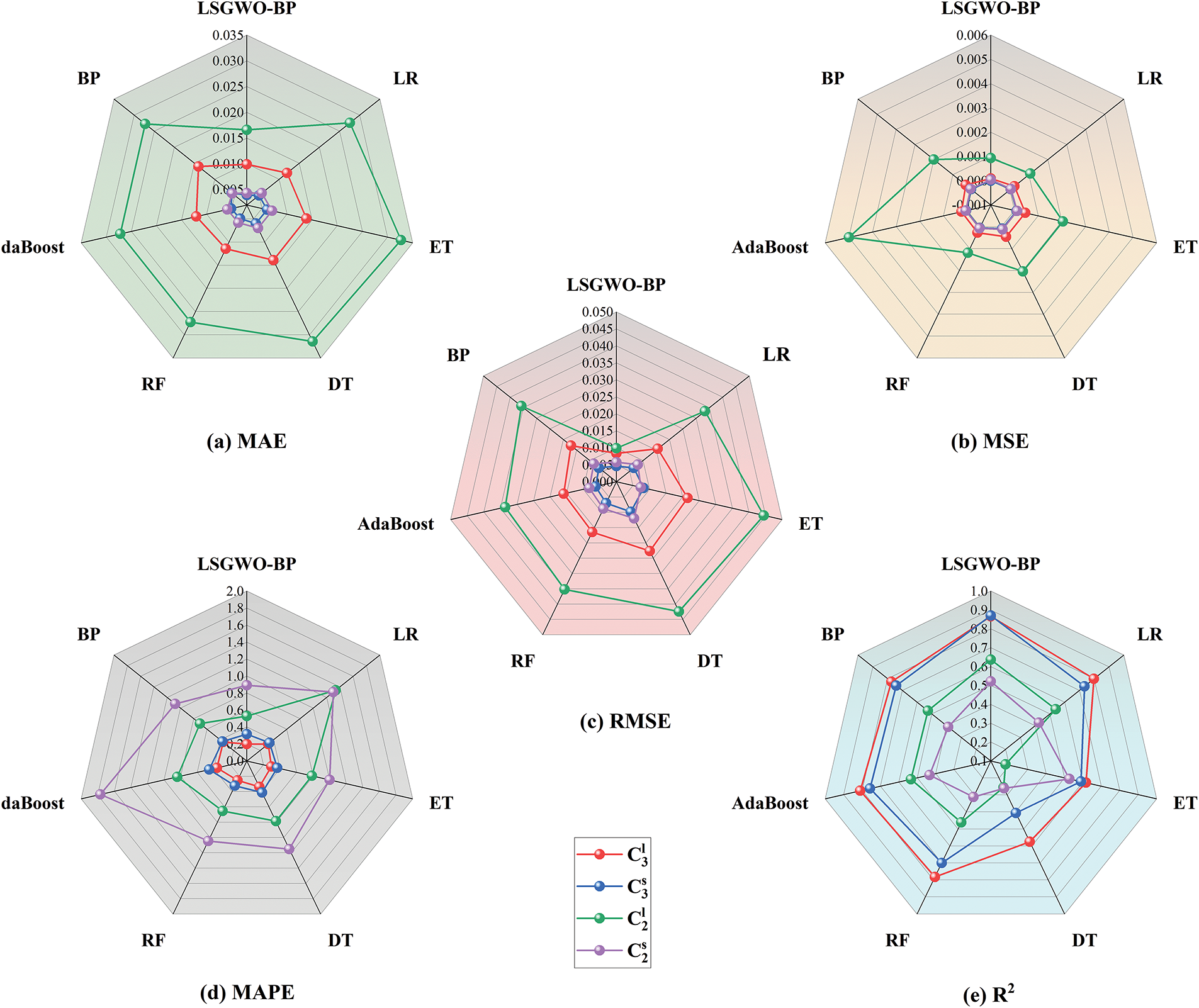
Figure 20: Radar chart of error metrics for each model

LSGWO-BP outperforms the other six traditional machine learning models in the results of five evaluation metrics and in the comparison plots between predicted and actual values. This advantage arises from the integration of the BP neural network and the improved GWO algorithm in LSGWO-BP, enabling the neural network to capture intricate data relationships. LSGWO optimizes the weights and biases of the BP neural network, enhancing its global search and local optimization capacities, which allows the model to adapt better to diverse dataset features, resulting in improved predictive accuracy and robustness. The multi-layer structure of the neural network autonomously learns complex feature representations from data, enabling LSGWO-BP to excel in processing high-dimensional and complex data. Additionally, regarding feature processing capability, the BP neural network autonomously learns and extracts nonlinear features through hidden layers without requiring manual handling, making it particularly advantageous for datasets with diverse and complex characteristics. In terms of parameter optimization, the LSGWO algorithm performs a global search by simulating the hunting behavior of grey wolves, effectively avoiding local optima and enabling the BP neural network parameters to achieve global optimality. LSGWO also dynamically adjusts neural network parameters, ensuring the model maintains robust predictive performance across various datasets. The LSGWO algorithm enhances the BP neural network model’s adaptability to different data characteristics, resulting in stronger generalization ability, greater stability, and more accurate predictions for LSGWO-BP across different datasets.

In summary, based on the above analysis, LSGWO-BP has significant advantages in terms of model structure, feature processing capability, parameter optimization, and adaptability to data characteristics. This results in a better fit between predicted and actual values compared to traditional machine learning models, demonstrating the excellent performance of LSGWO-BP in handling complex data.

4  Conclusion

This study introduces an optimized machine learning model–a BP neural network optimized by a GWO algorithm enhanced through Logistic-Sine chaotic mapping. The model is designed to predict the quasi-phase equilibrium of Al-Cu-Mg ternary alloys within the KKS phase-field model.

(1) The Logistic-Sine mapping mechanism improves the diversity of the initial population and enhances the global search capability of the GWO algorithm, thereby avoiding entrapment in local optima and increasing the algorithm’s adaptability and robustness when addressing large-scale, complex datasets.

(2) The LSGWO-BP model integrates the deep learning capacity of BP neural networks with the global optimization ability and convergence efficiency of the improved GWO algorithm, resulting in significantly enhanced predictive performance.

(3) A comprehensive performance evaluation of the LSGWO-BP model was conducted for the KKS phase-field modeling of multicomponent alloys, including simulations of metallic microstructure morphology under various conditions. Experimental validation confirms that the model maintains high predictive accuracy and stability even when accounting for compositional complexity and microstructural variation. Statistical analyses further demonstrate the model’s potential in multicomponent alloy phase-field simulations, highlighting its advantages as a highly efficient and reliable predictive tool.

Acknowledgement: The authors are deeply grateful to all team members involved in this research. Special thanks are extended to the anonymous reviewers and editors for their constructive feedback and meticulous review, which greatly improved the quality of this work.

Funding Statement: This work is supported by the National Natural Science Foundation of China (Grant Nos. 52161002, 51661020 and 11364024)

Author Contributions: Changsheng Zhu: Conceptualization, Methodology, Software, Supervision, Investigation. Jintao Miao: Data curation, Visualization, Writing—original draft, Formal analysis, Writing—review & editing, Software, Validation. Zihao Gao: Investigation, Supervision, Validation, Software. Shuo Liu: Software, Validation, Supervision. Jingjie Li: Software, Validation, Supervision. All authors reviewed the results and approved the final version of the manuscript.

Availability of Data and Materials: Data available on request from the authors.

Ethics Approval: Not applicable.

Conflicts of Interest: The authors declare no conflicts of interest to report regarding the present study.

References

1. Jiang X, Zhang R, Zhang C, Yin H, Qu X. Fast prediction of the quasi phase equilibrium in phase field model for multicomponent alloys based on machine learning method. Calphad. 2019;66:101644. doi:10.1016/j.calphad.2019.101644. [Google Scholar] [CrossRef]

2. Chen L-Q. Phase-field models for microstructure evolution. Annu Rev Mater Res. 2002;32(1):113–40. doi:10.1146/annurev.matsci.32.112001.132041. [Google Scholar] [CrossRef]

3. Steinbach I. Phase-field models in materials science. Model Simul Mater Sci Eng. 2009;17(7):073001. doi:10.1088/0965-0393/17/7/073001. [Google Scholar] [CrossRef]

4. Moelans N, Blanpain B, Wollants P. An introduction to phase-field modeling of microstructure evolution. Calphad. 2008;32(2):268–94. doi:10.1016/j.calphad.2007.11.003. [Google Scholar] [CrossRef]

5. Plapp M. Unified derivation of phase-field models for alloy solidification from a grand-potential functional. Phy Rev E. 2011;84(3):031601. doi:10.1103/PhysRevE.84.031601. [Google Scholar] [PubMed] [CrossRef]

6. Wang YU, Jin YM, Khachaturyan AG. Phase field microelasticity theory and modeling of elastically and structurally inhomogeneous solid. J Appl Phys. 2002;92(3):1351–60. doi:10.1063/1.1492859. [Google Scholar] [CrossRef]

7. Boettinger WJ, Warren JA, Beckermann C, Karma A. Phase-field simulation of solidification. Annu Rev Mater Res. 2002;32(1):163–94. doi:10.1146/annurev.matsci.32.101901.155803. [Google Scholar] [CrossRef]

8. Tourret D, Liu H, Llorca J. Phase-field modeling of microstructure evolution: recent applications, perspectives and challenges. Prog Mater Sci. 2022;123:100810. doi:10.1016/j.pmatsci.2021.100810. [Google Scholar] [CrossRef]

9. Zhang C, Yang Y. The CALPHAD approach for HEAs: challenges and opportunities. MRS Bull. 2022;47(2):158–67. doi:10.1557/s43577-022-00284-8. [Google Scholar] [CrossRef]

10. Masuda T, Sauvage X, Hirosawa S, Horita Z. Achieving highly strengthened Al–Cu–Mg alloy by grain refinement and grain boundary segregation. Mate Sci Eng A. 2020;793:139668. doi:10.1016/j.msea.2020.139668. [Google Scholar] [CrossRef]

11. Zeng H, Ai X, Chen M, Hu X. Application of phase field model coupled with convective effects in binary alloy directional solidification and roll casting processes. Front Mater. 2022;9:989040. doi:10.3389/fmats.2022.989040. [Google Scholar] [CrossRef]

12. Rakhmonov J, Liu K, Pan L, Breton F, Chen X. Enhanced mechanical properties of high-temperature-resistant Al-Cu cast alloy by microalloying with Mg. J Alloys Comp. 2020;827:154305. doi:10.1016/j.jallcom.2020.154305. [Google Scholar] [CrossRef]

13. He X, Lv S, Dou R, Zhang Y, Wang J, Liu X, et al. Microstructure and hot tearing sensitivity simulation and parameters optimization for the centrifugal casting of Al-Cu alloy. Comput Mater Contin. 2023;80(2):2873–95. doi:10.32604/cmc.2024.052571. [Google Scholar] [CrossRef]

14. Peivaste I, Siboni NH, Alahyarizadeh G, Ghaderi R, Svendsen B, Raabe D, et al. Machine-learning-based surrogate modeling of microstructure evolution using phase-field. Comput Mater Sci. 2022;214(1):111750. doi:10.1016/j.commatsci.2022.111750. [Google Scholar] [CrossRef]

15. Lookman T, Balachandran PV, Xue D, Yuan R. Active learning in materials science with emphasis on adaptive sampling using uncertainties for targeted design. npj Comp Mater. 2019;5(1):21. doi:10.1038/s41524-019-0153-8. [Google Scholar] [CrossRef]

16. Montes de Oca Zapiain D, Stewart JA, Dingreville R. Accelerating phase-field-based microstructure evolution predictions via surrogate models trained by machine learning methods. npj Comp Mater. 2021;7(1):3. doi:10.1038/s41524-020-00471-8. [Google Scholar] [CrossRef]

17. Yang J, Harish S, Li C, Zhao H, Antous B, Acar P. Deep reinforcement learning for multi-phase microstructure design. Comput Mater Contin. 2021;68(1):1285–302. doi:10.32604/cmc.2021.016829. [Google Scholar] [CrossRef]

18. Jaliliantabar F. Thermal conductivity prediction of nano enhanced phase change materials: a comparative machine learning approach. J Energy Storage. 2022;46(10):103633. doi:10.1016/j.est.2021.103633. [Google Scholar] [CrossRef]

19. Hu C, Martin S, Dingreville R. Accelerating phase-field predictions via recurrent neural networks learning the microstructure evolution in latent space. Comput Methods Appl Mech Eng. 2022;397(3):115128. doi:10.1016/j.cma.2022.115128. [Google Scholar] [CrossRef]

20. Fuhr AS, Sumpter BG. Deep generative models for materials discovery and machine learning-accelerated innovation. Front Mater. 2022;9:865270. doi:10.3389/fmats.2022.865270. [Google Scholar] [CrossRef]

21. Fan S, Hitt AL, Tang M, Sadigh B, Zhou F. Accelerate microstructure evolution simulation using graph neural networks with adaptive spatiotemporal resolution. Mach Learn: Sci Technol. 2024;5(2):025027. doi:10.1088/2632-2153/ad3e4b. [Google Scholar] [CrossRef]

22. Kim SG, Kim WT, Suzuki T. Phase-field model for binary alloys. Phys Rev E. 1999;60(6):7186. doi:10.1103/PhysRevE.60.7186. [Google Scholar] [PubMed] [CrossRef]

23. Buhler T, Fries SG, Spencer PJ, Lukas HL. A thermodynamic assessment of the Al–Cu–Mg ternary system. J Phase Equilibria. 1998;19(4):317–33. doi:10.1361/105497198770342058. [Google Scholar] [CrossRef]

24. Schmidhuber J. Deep learning in neural networks: an overview. Neural Netw. 2015;61(3):85–117. doi:10.1016/j.neunet.2014.09.003. [Google Scholar] [PubMed] [CrossRef]

25. Makhadmeh SN, Al-Betar MA, Doush IA, Awadallah MA, Kassaymeh S, Mirjalili S, et al. Recent advances in Grey Wolf Optimizer, its versions and applications: review. IEEE Access. 2024;12(3):22991–3028. doi:10.1109/ACCESS.2023.3304889. [Google Scholar] [CrossRef]

26. Demir FB, Tuncer T, Kocamaz AF. A chaotic optimization method based on logistic-sine map for numerical function optimization. Neural Comput Appl. 2020;32(17):14227–39. doi:10.1007/s00521-020-04815-9. [Google Scholar] [CrossRef]

27. Geurts P, Ernst D, Wehenkel L. Extremely randomized trees. Mach Learn. 2006;63(1):3–42. doi:10.1007/s10994-006-6226-1. [Google Scholar] [CrossRef]

28. Probst P, Wright MN, Boulesteix A‐L. Hyperparameters and tuning strategies for random forest. Wiley Interdiscip Rev: Data Min Know Disc. 2019;9(3):e1301. doi:10.1002/widm.1301. [Google Scholar] [CrossRef]

29. Collins M, Schapire RE, Singer Y. Logistic regression, AdaBoost and Bregman distances. Mach Learn. 2002;48(1/3):253–85. doi:10.1023/A:1013912006537. [Google Scholar] [CrossRef]

30. Karlsson A. Introduction to linear regression analysis. J Royal Statist Soc Ser A-Statist Soc. 2007;170(3):856–7. doi:10.1111/j.1467-985X.2007.00485_6.x. [Google Scholar] [CrossRef]

31. Xu M, Watanachaturaporn P, Varshney PK, Arora MK. Decision tree regression for soft classification of remote sensing data. Remote Sens Environ. 2005;97(3):322–36. doi:10.1016/j.rse.2005.05.008. [Google Scholar] [CrossRef]

32. Jain M, Saihjpal V, Singh N, Singh SB. An overview of variants and advancements of PSO algorithm. Appl Sci. 2022;12(17):8392. doi:10.3390/app12178392. [Google Scholar] [CrossRef]

33. Chen Y-J, Huang H, Chen Z-S. AVOA-optimized CNN-BILSTM-SENet framework for hydrodynamic performance prediction of bionic pectoral fins. Ocean Eng. 2025;327(11):121002. doi:10.1016/j.oceaneng.2025.121002. [Google Scholar] [CrossRef]

34. Chen X, Cheng L, Liu C, Liu Q, Liu J, Mao Y, et al. A WOA-based optimization approach for task scheduling in cloud computing systems. IEEE Syst J. 2020;14(3):3117–28. doi:10.1109/JSYST.2019.2960088. [Google Scholar] [CrossRef]

35. Zhou J, Huang S, Qiu Y. Optimization of random forest through the use of MVO, GWO and MFO in evaluating the stability of underground entry-type excavations. Tunnell Undergr Space Technol. 2022;124(12):104494. doi:10.1016/j.tust.2022.104494. [Google Scholar] [CrossRef]