Intelligent Estimation of ESR and C in AECs for Buck Converters Using Signal Processing and ML Regression

1  Introduction

Climate change is having an increasing impact on our lives, making it more crucial than ever to reduce greenhouse gas emissions. In this regard, generating clean energy from renewable sources, particularly electricity, is key.

According to Eurostat, electricity is the second-largest energy source after oil and petroleum products, accounting for 23% of final energy consumption in the European Union in 2022 [1]. This is supported by the International Energy Agency’s report, “Electricity 2024” [2], which states that the final consumption of electrical energy is projected to reach 20% in 2023, up from 18% in 2015. This highlights the growing trend toward electrification as a means to achieve global decarbonization goals.

The accelerated shift towards widespread electrification is reshaping all sectors of the economy. In the primary sector, the adoption of electric and hybrid vehicles [3], as well as drones and robots [4,5], is increasing efficiency and reducing environmental impact. Industrial electrification has become an irreversible trend [6,7], ensuring improved energy efficiency and reduced greenhouse gas emissions. On the other hand, sectors such as transport, retail, and healthcare are also undergoing rapid transformation, with the increasingly widespread use of electric vehicles (EVs) in public transport systems [8,9], as well as the increasingly widespread use of advanced, energy-efficient equipment in healthcare [10] and retail [11]. In this context, power converters (PCs) play a crucial role by facilitating the transfer of energy from the primary source to the load. Therefore, the increasing use of PCs in diverse and often critical applications underscores the growing importance of developing fault diagnosis techniques (FDT) to ensure the reliability and safety of their host systems.

PCs typically include switches, lossless energy storage components, and magnetic transformers. One of the lossless energy storage components in PCs is the capacitor, which, unfortunately, is also one of the most vulnerable elements of these systems [12]. This highlights the importance of fault diagnosis for capacitors in power converters, especially considering that these converters are integral to critical systems such as transportation vehicles [13], data centers [14], and medical equipment [15].

1.1 Aluminum Electrolytic Capacitors (AECs)

Among the capacitors used in power converters, aluminum electrolytic capacitors (AECs) are one of the most commonly used technologies, prized for their high volumetric efficiency and cost-effectiveness, as well as their availability in a range of capacities and sizes [12].

The basic structure of AECs includes a wound element (Fig. 1a) that is impregnated with an electrolyte. This core component is connected to external terminals and enclosed in a metal can (Fig. 1b). The element is formed by two aluminum foils serving as electrodes, the anode and the cathode, separated by paper separators soaked in electrolyte to avoid direct contact between the foils (Fig. 1a).

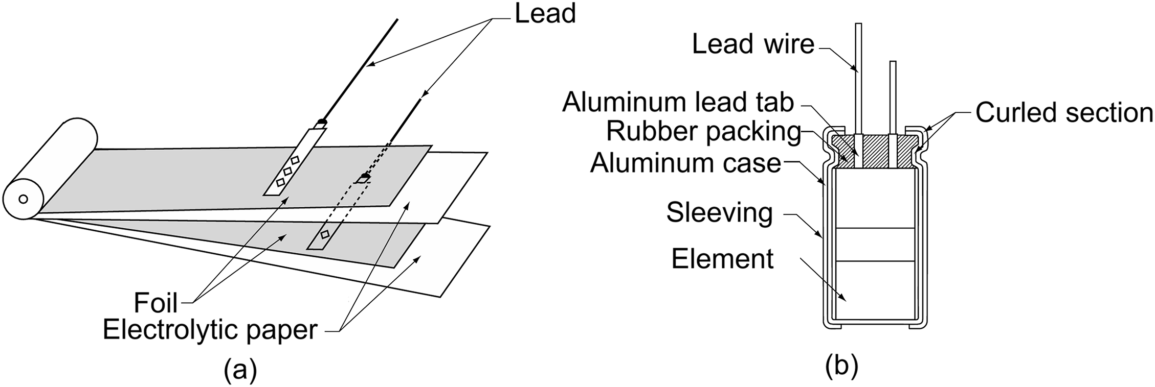
Figure 1: Basic structure of an AEC [16]: (a) the whole structure and (b) inside the can

Inside the AEC, there are two capacitors: the anode capacitor (an-C), made up of the anode foil, a dielectric layer designed to withstand the rated voltage, and the electrolyte; and the cathode capacitor (ca-C), which consists of the electrolyte acting as the positive plate, a very thin dielectric layer, and the cathode foil.

The electrolyte in an AEC serves multiple purposes: it promotes strong adhesion to the surfaces of both layers, maintains electrical continuity between an-C and ca-C, and helps repair defects in the anode’s dielectric layer. Strong adhesion is crucial to achieving high capacitance, while electrical continuity ensures effective conduction between the two internal capacitors. When defects form in the dielectric layer, leakage currents can trigger the electrolysis of water in the electrolyte, producing gases such as hydrogen and oxygen. Oxygen plays a key role in regenerating the dielectric in damaged areas. This process, referred to as self-healing, alters the electrical characteristics of the AEC. As the water content in the electrolyte decreases, the effective dielectric contact area decreases, resulting in a reduction of the capacitor’s capacitance (C). At the same time, the electrical conductivity between an-C and ca-C decreases, thus increasing the AEC’s equivalent series resistance (ESR).

Additional factors, such as high operating temperatures and high ripple currents, can accelerate the evaporation of the electrolyte, resulting in effects similar to those previously described.

The above failure mechanisms represent a parametric failure that can eventually lead to a catastrophic one [17,18], which can manifest itself as an open circuit. As a result, the operation of the converter is severely affected [12,18].

There is a limit beyond which increases in ESR or decreases in C should not be exceeded. Therefore, AEC manufacturers set limits that, if exceeded, significantly increase the risk of catastrophic failure. For ESR, the limit is twice the initial value of a healthy capacitor, while for C, it is 80% of the value of a sound capacitor [12,18].

1.2 Comprehensive Overview of Fault Diagnosis Techniques (FDTs) for AECs

The literature on this topic is extensive and dates back more than 20 years, with its relevance increasing in recent years due to the widespread adoption of these converters. Fault diagnosis techniques (FDT) can be classified based on the operational or conceptual perspective [19].

From an operational perspective, three main types of fault diagnosis techniques (FDT) are recognized [12,19]: offline techniques (OFF-FDT), quasi-online techniques (QON-FDT), and online techniques (ON-FDT). The OFF-FDTs require the removal of the capacitor from the original circuit (power converter) and its placement in a test circuit. Test circuits produce the necessary currents and voltages to characterize the equivalent circuit of the device being tested. This straightforward method reduces errors and enables precise measurement of capacitor ESR and capacitance values under particular operating conditions. Nevertheless, removing the capacitor from the converter proves impractical in most cases. In QON-FDT, the capacitor remains in the converter during testing, but its condition is evaluated during a routine pause in the application [20]. During this period, an unconventional operation is introduced, which could be imposed by injecting an external signal, applying a special operational configuration, or both [12,20]. The ON-FDT design becomes crucial for applications that require uninterrupted operation, particularly in critical systems. Here, the AEC status evaluation occurs in real time without disrupting converter functionality. This method enables more effective planning of maintenance schedules based on predictive analysis, thereby reducing the risk of unexpected system failures [12,19].

This paper focuses on ON-FDT and provides an overview of key solutions for fault diagnosis in AECs. As mentioned earlier, ON-FDT can be classified from a conceptual perspective into three categories: signal-based (SB-ON-FDT), model-based (MB-ON-FDT), and data-based (DB-ON-FDT) Fault Diagnosis Techniques [19]. SB-ON-FDT rely on measured signals, from which key features are extracted using signal processing techniques (SPT) [21–23]. The features extracted from the raw signals show distinct patterns that depend on the severity of the failure. By examining these patterns, it is possible to identify relationships between various signal characteristics, which helps determine the level of failure severity. Features can be extracted from signals using time-domain methods, frequency-domain methods, or combined approaches that use elements from both techniques [12,21–23]. The SB-ON-FDT implementation does not require knowledge of the converter parameters, doesn’t need large datasets for model training, and provides a quick response [12,23]. However, it usually requires integrating additional sensors into the system [19]. The MB-ON-FDTs depend on the mathematical model (MM) representing the system, and a discrepancy between the MM’s output and the actual physical system data may indicate a failure. This method requires a thorough understanding of the system MM, unlike the SB and DB approaches [21,23,24]. Through raw data analysis, DB-ON-FDT can assess the health status of the AECs. To achieve this, it is necessary to create a training dataset from which ML models can learn fault detection patterns [19].

In [25], the authors proposed an SB-ON-FDT for a flyback DC-DC converter. To implement their approach, they assume the capacitor current waveform is approximately square and neglect the capacitor’s inductive effect. Based on these assumptions, they derived two analytical expressions to estimate the ESR value, using some signals features such as the mean value of the output voltage ripple during conduction stage, the mean value of capacitor current during conduction stage, the output voltage ripple halfway the conduction stage, the mean value of output current, the duty cycle and the switching period. Subsequently, in [26], a new SB-ON-FDT is introduced that employs a new analytical relationship between the output voltage ripple and the input current for boost and buck-boost converters. Its primary advantage is that it is non-invasive. In [27], the authors present an invasive method to estimate the ESR value by deriving an analytical relationship between the average power dissipated by the capacitor and the root-mean-square (RMS) value of its current. The approaches outlined above extract signal features that enable ESR estimation using time-domain approaches.

In [28], the authors introduce an electronic module designed to indicate when the capacitor in the output filter of a PC needs replacement. The ESR value prediction is achieved through a simple relationship between the fundamental components of the capacitor’s voltage and current. If the estimated value is twice that of a reference system representing a sound capacitor, replacement is recommended. Later [29], the authors utilize analytical relationships between the characteristics of the current and voltage signals in the capacitor to estimate the ESR and C values of AEC simultaneously. Signal features are extracted using the Goertzel algorithm. In [22], the authors introduce a new method for analyzing capacitor current and voltage signals by combining the discrete wavelet transform (DWT) with a sliding window to compute the RMS value. Using this characteristic, the ESR and C values are then determined through straightforward analytical formulas. Lastly, the capacitor’s condition is assessed by comparing the ratio of the current ESR and C values to those of a sound capacitor, with a Kalman filter applied to minimize noise effects. Later, in [30], the authors propose a solution that combines a 5th-order Butterworth filter with an RMS filter for ESR estimation. Instead of positioning the current sensor in the capacitor branch, as is typically done, they place it in the inductor branch and compute the capacitor current analytically using the output current, PWM signal, and inductor current. The methods described above extract signal features that enable the estimation of ESR and C using frequency-domain techniques, such as filters, the Goertzel algorithm, the Fast Fourier Transform (FFT), and the discrete wavelet transform (DWT).

The FDTs discussed in this paragraph fall under the MB-ON-FDT classification. The authors of [31] propose a solution based on the circuit model to estimate the ESR and C values of the AEC present in the PC’s output filter. PCs are hybrid dynamic systems, so it is possible to combine the state-space model with the Least Mean Squares (LMS) algorithm to extract the model coefficients, specifically the parameters inherent to the capacitors. Later, in [32], the authors combine the digital twin concept with an optimization algorithm to evaluate the health status of the capacitors in the output filter of a buck converter. They use the Particle Swarm Optimization (PSO) algorithm to estimate the circuit parameters, aiming to minimize the difference between the behavior of the digital twin and the physical system. Some of the estimated parameters naturally include the C and ESR values of the AEC.

The subsequently discussed FDTs fall under the DB-ON-FDT classification. Artificial neural network (ANN)-based schemes have been proposed for estimating capacitor parameters in adjustable-speed drives (ASD) [33–35]. Implementing deep learning models requires assembling a large training dataset that covers a broad range of operating conditions. Some solutions are framed as a regression problem aimed at estimating the value of C, with different features extracted from the sampled signals used as input to the ANN. In [33], the inputs to the ANN consist of the RMS values of the input and output currents and voltages, along with the DC link voltage. In [34], the number of ANN inputs is reduced to two: the RMS value of a single-phase output current and dc-link voltage ripple. Conversely, in [35], the authors utilize the DC link voltage harmonics in conjunction with the RMS value of a single-phase output current. In [36], the authors introduce a deep neural network (DNN)-based approach for estimating both ESR and C values of the input capacitor in a single-phase DC/AC power converter. Initially, feature extraction is performed on the capacitor voltage and current signals to isolate relevant spectral information. The extracted features comprise frequency components that are twice the fundamental frequency and twice the converter switching frequency, obtained through the Fast Fourier Transform (FFT). Since the authors formulate the problem as a regression task, the outputs of the DNN correspond to the estimated values of ESR and C. In [37], the authors view the problem as a multi-class classification task with three possible outcomes: normal operation, failure in the first capacitor, or failure in the second capacitor. They use an adaptive neuro-fuzzy inference system (ANFIS) to evaluate the health of two capacitors in a wind power system supplying a single-phase grid. The first capacitor is located at the output of the three-phase rectifier. At the same time, the second capacitor is positioned between the boost converter output and the input of a single-phase inverter. The ANFIS model takes only the converter input voltage and the DC filter output voltages as inputs. In [19], the authors use an autoencoder (AE) trained solely with data from a healthy 3ϕIBC, enabling the AE to reconstruct input signals accurately. Naturally, in healthy conditions, the reconstruction error remains low, but it increases significantly when the 3ϕIBC output filter contains aged capacitors. The AE inputs include the output voltage amplitude, load resistance, and average output voltage. The first attribute was obtained using the Short-Time Least Squares Prony (STLSP) algorithm. As the AE output, the authors use the reconstructed amplitude of the output voltage. To evaluate the capacitor’s condition, deviations in the reconstruction error are analyzed. Although previous solutions employed deep learning algorithms, they required pre-processing of the input data rather than working directly with raw signals. As a result, relevant features had to be extracted beforehand.

Recently, in [38], the authors introduced a novel DB-ON-FDT which utilizes raw data as input to a hybrid convolutional neural network-attention model (HCNN-AM). This deep learning model takes as input just the DC-link voltage of a three-phase PWM inverter with a front-end diode rectifier used for AC machine drives. Its primary goal is to assess the condition of the DC-link capacitor by treating the problem as a regression task, estimating both ESR and C values. The CNN component handles the feature selection task, while the attention mechanism estimates both ESR and C values based on those features.

In [39], the authors employed traditional machine learning algorithms, such as K-Nearest Neighbors (KNN), Support Vector Machine (SVM), and Naive Bayes (NB), to monitor the condition of the DC-link capacitor in a Back-to-Back (BTB) converter. The authors approach this problem as a multiclass classification with five categories: healthy, aged, critical, very critical, and high alarm. Features are derived from raw data using a combination of statistical measures and DWT. The raw data represents the voltage ripple across the DC link capacitor. In [40], the authors propose a method that leverages time-frequency analysis of conducted electromagnetic interference (EMI) to classify the health status of the DC-link capacitor in a three-phase inverter. The EMI signals are analyzed during switching events using the Continuous Wavelet Transform (CWT), which generates distinctive switching patterns. These patterns serve as input features for training an SVM model, enabling it to classify the capacitor’s condition into five severity levels. Later, in [41], the authors propose an FDT by treating it as a binary classification problem. To do this, they use a Logistic Regression (LR) model to determine whether the AEC in the output filter of a 3ϕIBC is healthy or faulty. The method does not rely on additional sensors, as the capacitor current is reconstructed from signals already available in the converter control system. First, the extraction of features from the reconstructed current and the capacitor voltage signals is obtained in the signal processing module. Finally, the LR model uses the features to classify the capacitor as either a sound AEC or an aged AEC after the training stage.

Finally, a brief comparison of the three conceptual FDT solutions is provided. Most SB-ON-FDTs rely on a current sensor in the capacitor branch, which can be impractical in many applications. Additionally, other SB-ON-FDTs require extra hardware circuitry. MB-ON-FDT techniques require high sampling frequencies, involve models with complex calculations, and depend on the topology of the converter being analyzed. It is also important to note that MB-ON-FDTs need the measurement of the converter’s internal state variables, making them inherently invasive. Lastly, DB-ON-FDTs, especially those using DL, deliver excellent performance but require extensive training datasets and significant computational resources for model training. The challenge of creating large datasets can be reduced if the approach proposed in this paper is adopted by simply adapting the pipeline to a DL model.

This paper proposes a novel solution to overcome the limitations mentioned above by combining signal processing techniques (SPT) with traditional machine learning models (TML) to assess the health status of capacitors used in the DC-link of PCs. Although TML models necessitate data preprocessing, unlike DL models, they provide substantial benefits, including significantly reduced training data requirements and considerably lower computational costs. Furthermore, this approach enables the implementation of non-invasive and efficient FDTs, as it utilizes features extracted from the converter’s input and output signals. In contrast, the SB-ON-FDT and MB-ON-FDT methods require the introduction of sensors within the converter.

Specifically, a linear regression model is employed to estimate both the ESR and C of AEC used in the buck converter output filter. The method relies solely on the input and output current and the output voltage of the converter, making it a non-invasive approach. The computational cost of the proposed solution is minimal, and this issue arises only during the training stage, as linear regression produces a mathematical equation that represents the relationship between the model’s output and inputs. To enhance model performance, feature engineering was applied to generate new features from the original ones.

The proposed approach aims to deliver a solution that is computationally lightweight, non-invasive, and scalable, making it suitable for practical deployment in real-world applications.

2  Raw Data Generation and Preprocessing Pipeline

This section outlines the complete process of raw data generation and subsequent processing used to construct the original dataset.

Initially, the buck converter was simulated under various operating conditions using the method proposed in [42]. This method enables the simulation of a buck converter in Python and has been validated against LTspice simulation software, a powerful tool often used in academia and industry for its accuracy in simulating electrical circuits [42]. This method was selected due to its ability to efficiently and automatically run multiple sequential simulations across a wide range of operational scenarios. Besides simplifying the simulation process, it is highly scalable, making it ideal for creating datasets tailored for machine learning (ML) algorithms. A thorough description of this simulation approach is included in the reference [42].

To ensure that the simulated behavior closely mirrors that of a commercial buck converter, a set of 625 different operating condition ranges was randomly defined. Specifically, the duty cycle (D) and load resistance (R) values were generated to approximate a normal distribution. For the load resistance, a mean of 1 Ω with a standard deviation of 0.3 was used, constrained between 0.4 and 1.6 Ω (Fig. 2). For the duty cycle, a mean of 0.5 and a standard deviation of 0.15 were applied, with values limited between 0.1 and 0.9 (Fig. 2). The following figure presents histograms of both distributions, which demonstrate a close resemblance to the normal distribution.

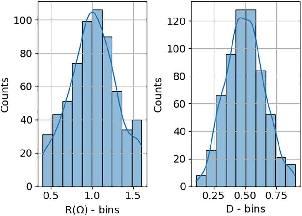
Figure 2: Range of randomly defined operating conditions, where R denotes the load resistance and D the duty cycle

After establishing the operational conditions, the method for extracting features from the raw data was defined, utilizing the solution proposed in [30], which enabled the calculation of the RMS value of a signal after filtering and applying a sliding window. The signal processing framework that enables the extraction of pertinent features from the input signals is fully described in reference [30].

Fig. 3 summarizes the key steps of the signal processing algorithm used to generate the features that serve as inputs to the ML model.

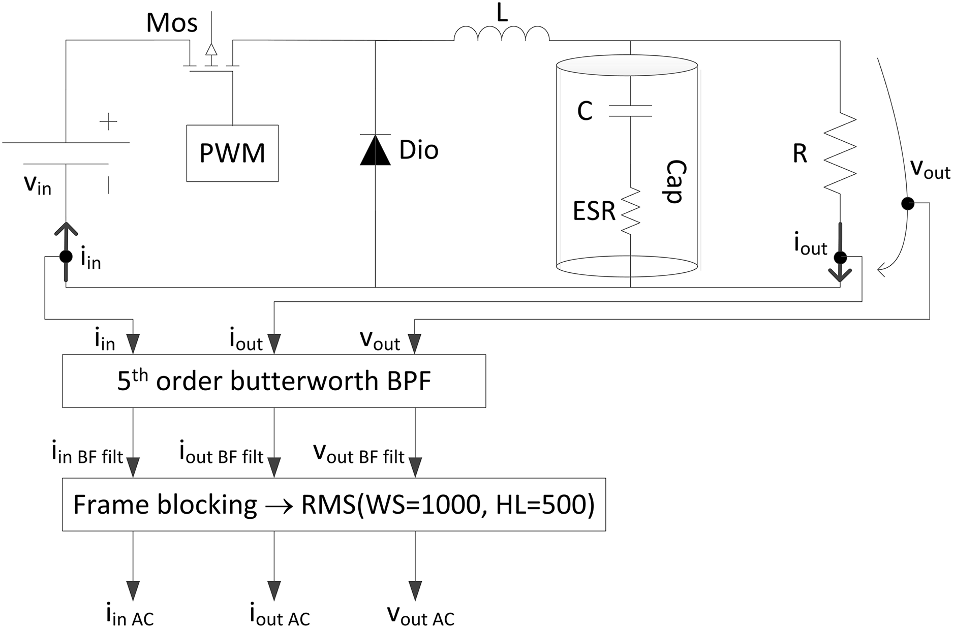
Figure 3: Buck converter schematics and key steps of the signal processing (SP) algorithm used to extract features from raw data

Fig. 3 illustrates the schematic of a buck converter, which comprises two semiconductor devices: a diode (Dio) and an MOS transistor (Mos), as well as two reactive components: an inductor (L) and a capacitor (Cap). The converter works on the principle that when the transistor conducts, the diode does not, allowing current to flow through the inductor and the capacitor, both of which store energy. When the transistor stops conducting, the stored energy in the inductor and capacitor is transferred to the load (R).

Fig. 3 demonstrates that the proposed solution is non-invasive, as it does not require inserting sensors directly into the circuit to measure the signals of interest: input current (iin), output current (iout), and output voltage (vout). Once these signals are acquired, they undergo a processing pipeline to extract features for input into the ML algorithm. Initially, the signals are passed through a band-pass filter that isolates the spectral components corresponding to the converter’s switching frequency (fsw). The band-pass filter comprises a low-pass filter with a 25 kHz cutoff frequency and a high-pass filter with a 15 kHz cutoff frequency. Next, the root mean square (RMS) value of the filtered signals is computed using a sliding window approach with a window size of 1000 samples and a hop size of 500 samples. The converter operates at a switching frequency of 20 kHz, while the sampling frequency is set to 20 MHz.

To illustrate the simulation process and the complete signal processing pipeline, the scenario outlined in Table 1 was considered, which details the electrical parameters of the buck converter used in this simulation.

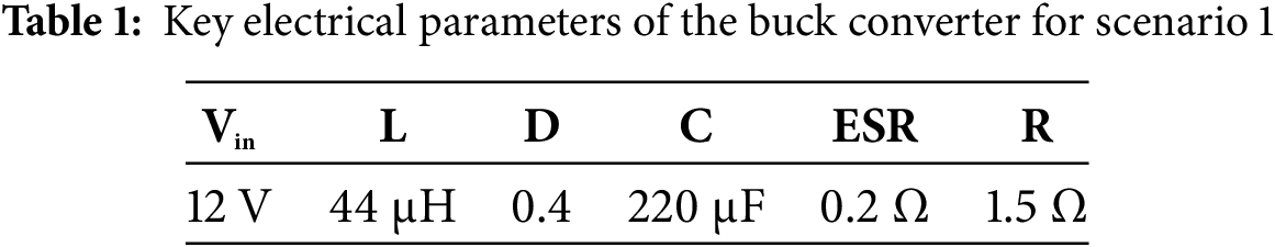
Fig. 4 presents the waveforms of the raw signals alongside their processed counterparts for scenario 1. The raw signals are labeled as input current (iin), output current (iout), and output voltage (vout), while the signal features, representing the root mean square (RMS) values of the filtered signals, are denoted as iinAC, ioutAC, and voutAC.

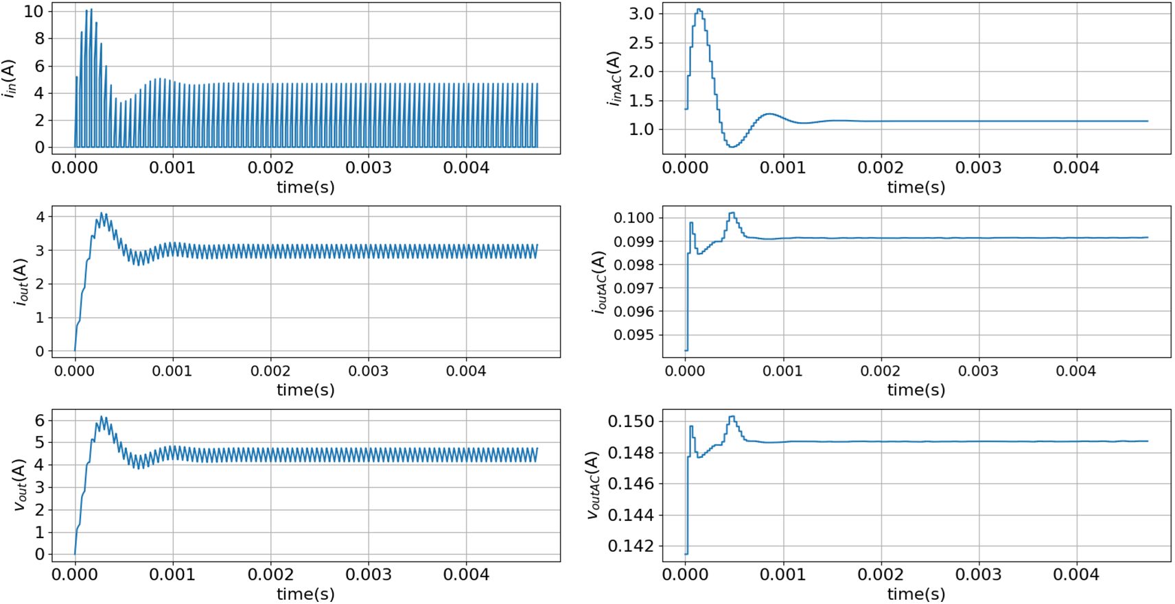
Figure 4: Input current, output current, and output voltage waveforms for scenario 1 (Table 1): raw data (iin, iout, and vout) and AC signals features or RMS value of the filtered signals (iinAC, ioutAC, and voutAC)

The previously mentioned features capture high-frequency signal characteristics, hence, the use of the ‘AC’ prefix. To extract information related to lower frequencies, closer to the DC component, additional features were derived from the same signals. This was achieved by applying a moving average filter to the signals, using sliding windows of 1000 samples with a hop size of 500 samples (Fig. 5).

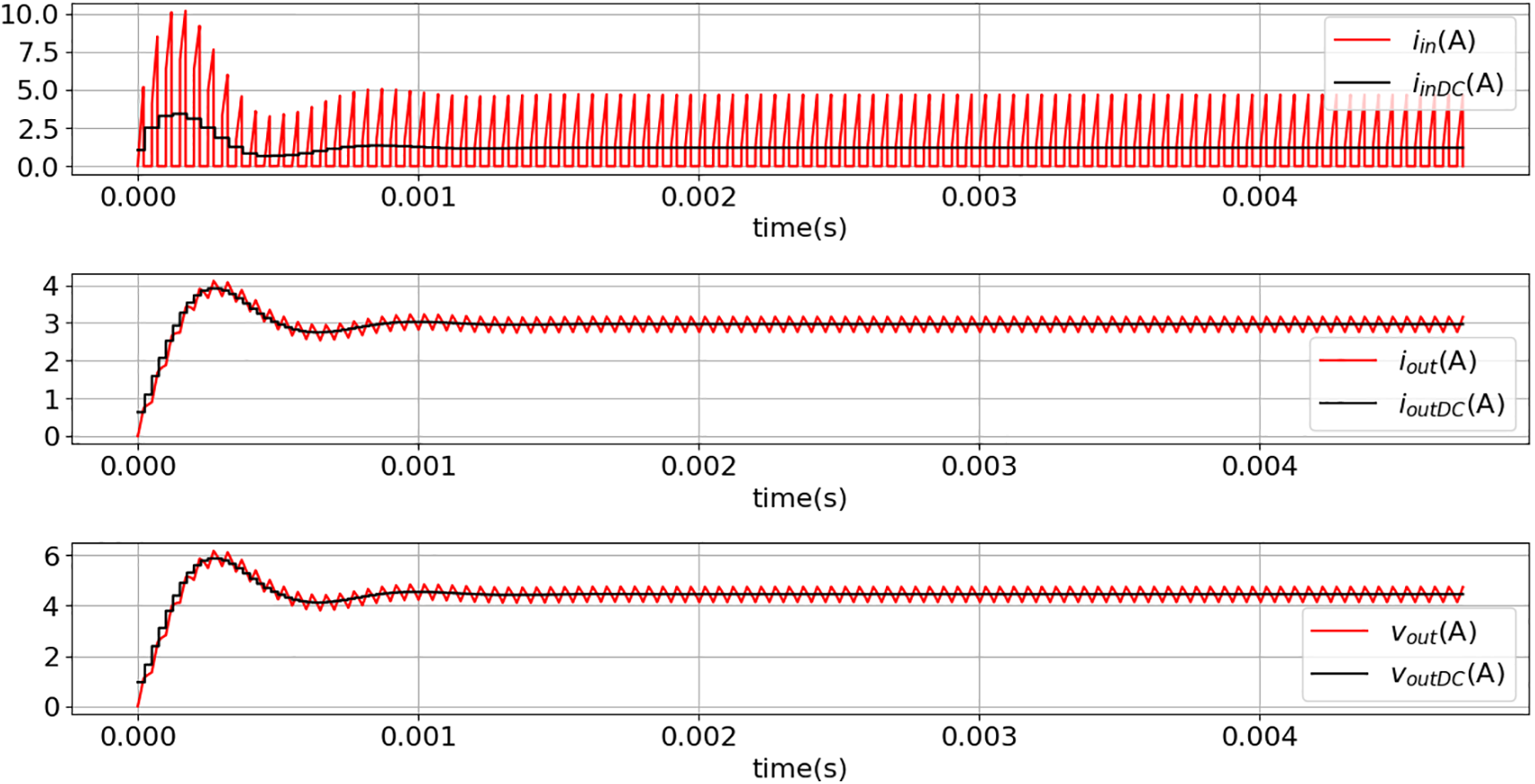
Figure 5: Input current, output current, and output voltage waveforms for scenario 1 (Table 1): raw data (iin, iout, and vout) and DC signals features or average value of the raw signals (iinDC, ioutDC, and voutDC)

As shown in Fig. 5, the low-frequency features were labeled with the ‘DC’ prefix.

For the model to accurately estimate the ESR and C of the AEC, the dataset should encompass data across multiple failure severity levels. For this purpose, five different severity levels (S0, S1, S2, S3, and S4) were considered (Fig. 6).

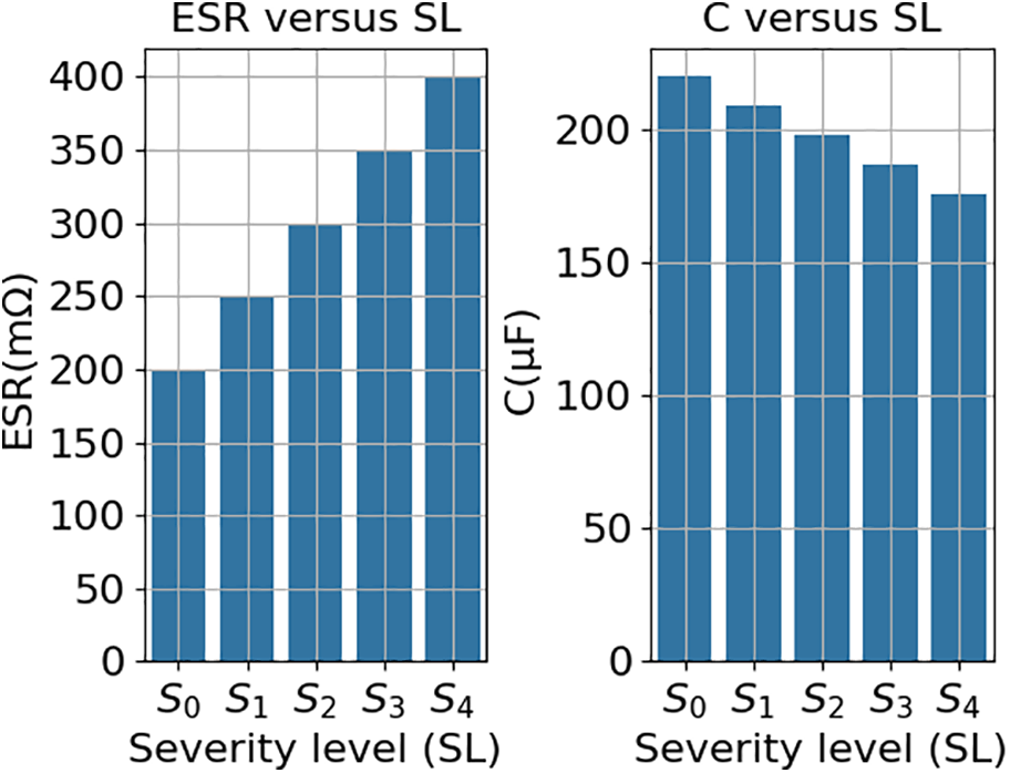
Figure 6: Severity levels vs. ESR and C values

Severity levels are defined based on the failure mechanisms outlined in Section 1.1. A higher ESR results in a decrease in C. AEC fails when ESR reaches twice the ESR of a sound AEC, which matches a 20% capacitance loss of a sound AEC.

Finally, after defining all the necessary requirements for the simulations, a total of 625 × 5 (3125) simulations were performed. For each simulation, a representative sample was extracted that contained the relevant signal features to feed the ML model. The values of the extracted features correspond to the median of the parameter set composed of iinAC, iinDC, ioutAC, ioutDC, voutDC, and voutAC. The parameters D, R, ESR, and C are unique values in each individual simulation.

The resulting dataset is illustrated in Fig. 7.

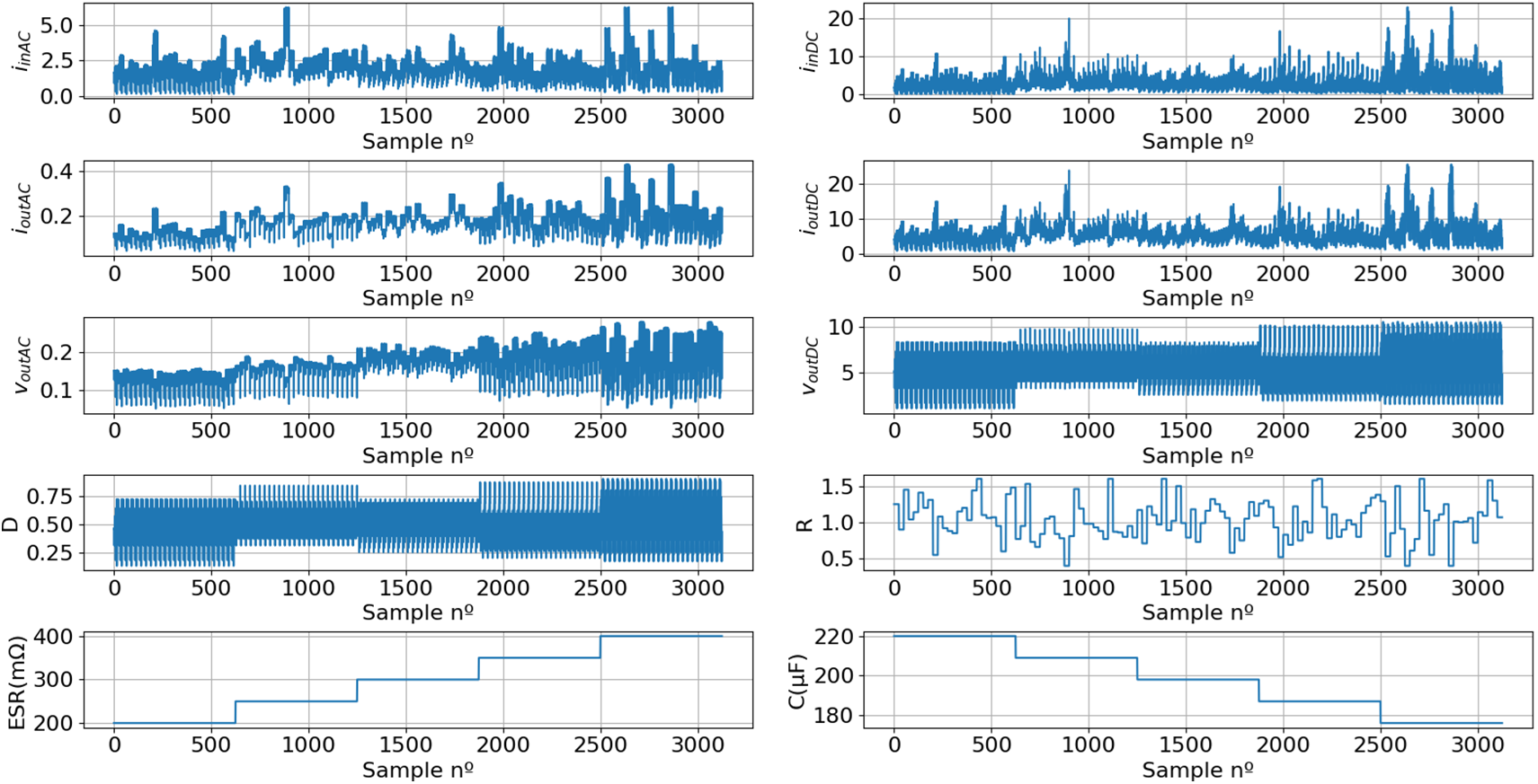
Figure 7: The original dataset, derived from 3125 simulations, contains all the features and target variables required for training the machine learning model

Fig. 7 introduces two new features: the duty cycle (D) and the load resistance (R). The value of D is provided directly by the PWM, eliminating the need for additional sensors. At the same time, R is calculated as the ratio of voutDC to ioutDC, also avoiding the need for extra sensing hardware.

3  Exploratory Data Analysis (EDA)

As previously stated, this paper aims to develop a fault diagnosis technique (FDT) that combines signal processing (SP) methods with machine learning (ML) algorithms for assessing the AEC condition. In essence, the proposed solution can be considered an ML-driven fault diagnosis project within the domain of electronics systems.

A typical ML project follows a series of clearly defined steps. The first two steps, which have already been discussed earlier, are problem definition and data collection. These are followed by exploratory data analysis (EDA), model training, validation, and finally, model deployment. This section focuses on the exploratory data analysis (EDA).

The EDA process begins with a clear understanding of the dataset, including the identification of its features and target variables. The original dataset contains eight numerical features: iinAC, iinDC, ioutAC, ioutDC, voutAC, voutDC, D, and R, as well as two numerical targets: ESR and C.

After identifying the variables, it is essential to review all dataset records to determine if further processing is needed, especially checking for duplicate or missing values. The original dataset has no missing or duplicate values; however, Fig. 7 indicates the presence of outliers in some features. Therefore, individual boxplots (Fig. 8) were created for each feature to visualize their distributions better.

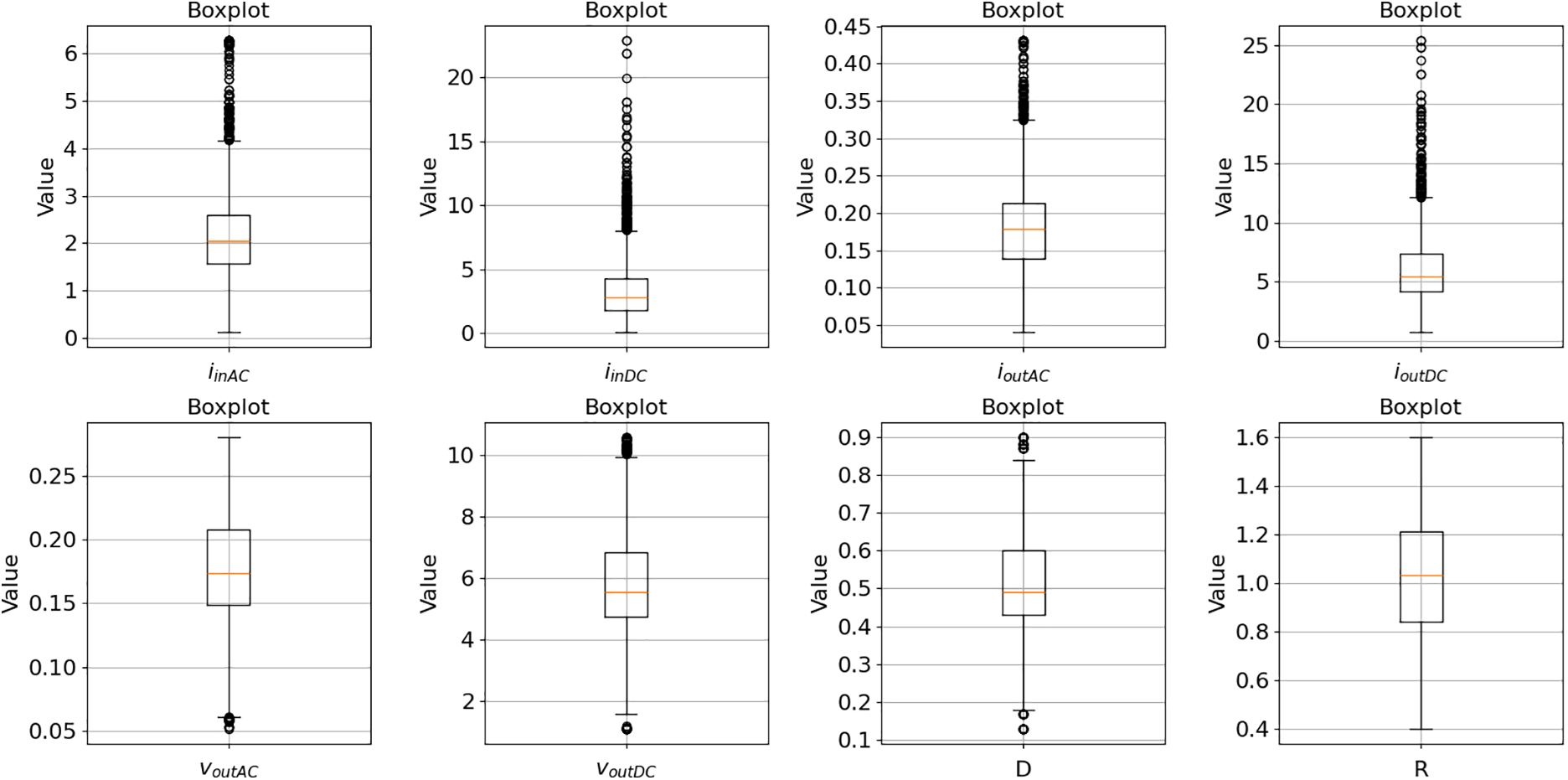
Figure 8: Individual boxplots regarding the features: iinAC, iinDC, ioutAC, ioutDC, voutAC, voutDC, D, and R

Fig. 8 reveals the presence of outliers, specifically in the currents, which will be retained in the dataset, as they may represent extreme operating conditions where the model is expected to identify the state of the AECs accurately.

The performance of an ML model is heavily influenced by the attributes used for prediction. Therefore, selecting the most relevant features is crucial for optimizing performance. Irrelevant attributes can increase model complexity and computation time, introduce noise, and potentially lead to overfitting. Therefore, Pearson’s correlation was applied to assess the relationships among the features and between each feature and the target variable, to identify and eliminate irrelevant features.

The Pearson correlation (r) between two variables X and Y can be computed using (1):

r=n×∑(X×Y)−∑X×∑Y(n×∑X2−(∑X)2)×(n×∑Y2−(∑Y)2)(1)

where n represents the number of samples.

Fig. 9 illustrates the correlations among the various features, as well as between the features and the target variables.

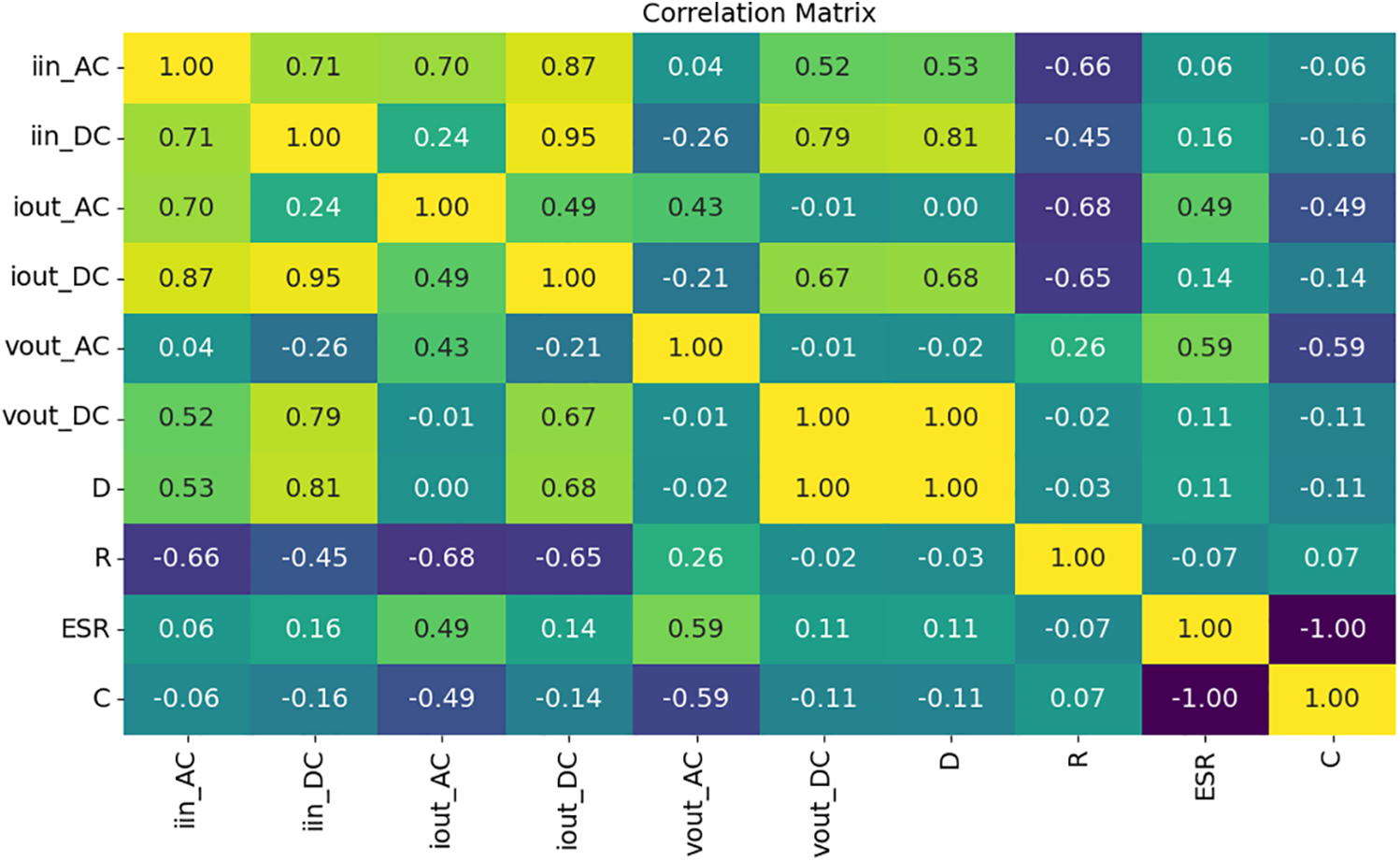
Figure 9: Correlation among variables

The correlation analysis presented in Fig. 9 reveals that the most significant independent variables relative to the targets are iout_AC and vout_AC, while the remaining features exhibit low correlations. Hence, to eliminate irrelevant variables, a correlation threshold of 0.9 was established. Whenever two features exceed this threshold, one of these variables should be removed. Naturally, priority was given to the feature with the strongest correlation with the target variables.

The features listed below exhibit strong correlations with other features:

•   iinDC is strongly correlated with ioutDC;

•   ioutDC is strongly correlated with iinDC;

•   voutDC is strongly correlated with D;

•   D is strongly correlated with voutDC.

Based on the previously defined requirements, it was decided to retain the following features: iinAC, iinDC, ioutAC, voutAC, voutDC, and R.

Figs. 7 and 8 reveal that the features operate on different scales. To ensure that all variables contribute equally to the model, normalization is essential. For this purpose, the min-Max scaling transformation (2) was applied.

Xnormalized=X−XminXmax−Xmin(2)

where X represents the actual feature value, Xmin the minimum value of X in the dataset, and Xmax the maximum value of X in the dataset.

Fig. 10 displays the descriptive statistics of the updated dataset after applying the min-max scaling transformation. As shown, all six features have been successfully scaled to the [0, 1] range. Moreover, except for the iinDC feature, the mean and median values of the remaining features are approximately equal, indicating a roughly symmetrical distribution of the data. Fig. 10 also shows that all features have a standard deviation greater than 0.1 or a variance exceeding 0.01, which is commonly used as the minimum threshold for excluding features.

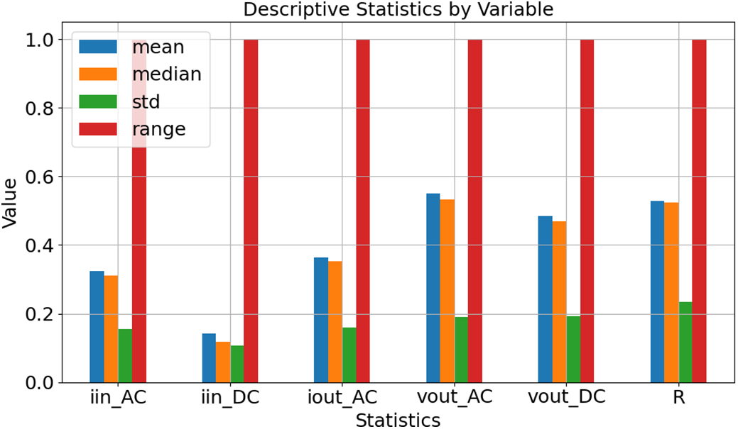
Figure 10: Descriptive statistics of the features after min-Max scaling transformation

Fig. 11 presents a histogram of all features, revealing that, except for iinDC, the other features exhibit an approximately normal distribution. For iinDC, the rightward skew of the histogram can be explained by the mean value being greater than the median.

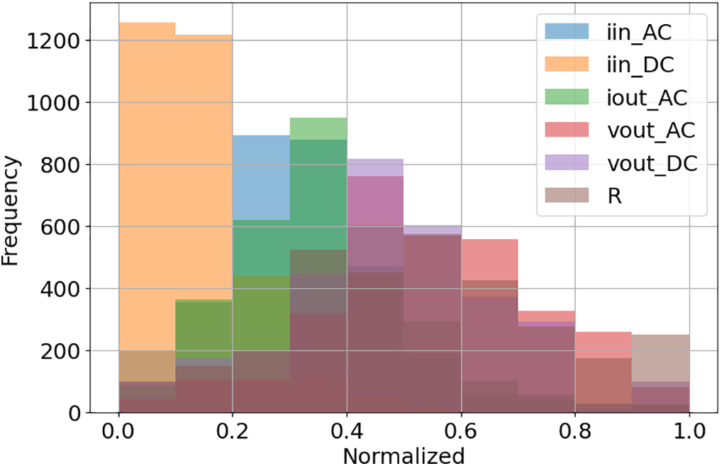
Figure 11: Histogram of all features after min-Max scaling transformation

4  Model Training and Evaluation—Linear Regression

This section introduces the first proposed solution, an ML algorithm known as linear regression. Before delving into the details, it is essential to provide some context on ML, which is generally categorized into three main types: supervised learning (SML), unsupervised learning (UML), and reinforcement learning (RML).

In SML, the model learns from labeled data; therefore, the training dataset includes both independent and dependent variables. In contrast, UML models learn solely from independent variables; the training data does not contain dependent variables or target values. RML algorithms learn by interacting with an environment, receiving rewards or penalties based on their actions to optimize future behavior.

Considering that the current study addresses a regression problem, specifically, developing a model to estimate the ESR and C values of AECs based on a set of independent variables, the proposed solution falls under the SML category.

SML algorithms learn to identify relationships between input features and target variables, enabling prediction on new, previously unseen data. The general form of an SML model can be expressed by (3):

ymodel=f(Xi,Kj)+E(3)

where:

∎   ymodel represents the dependent variable, target, or output. In the problem under analysis, ESR and C represent the dependent variables;

∎   Xi represents the i independent variable, feature, or input. In the problem under analysis, the features are: iinAC, iinDC, ioutAC, voutAC, voutDC and R;

∎   Kj represents the model’s parameters, which are estimated during the training stage;

∎   j denotes the number of parameters and represents one of the model’s hyperparameters, which can be configured to enhance the model’s performance. As will be shown in Section 5, increasing j from 6 to 27 enhances the model’s performance. Hyperparameters are typically adjusted through a process known as ML model tuning;

∎   E symbolizes the error between the model predictions and the actual response.

4.1 Six-Feature Linear Regression Model

The proposed models use the linear regression algorithm and can be expressed by the following equations:

{E⁢S⁢R⁡(F1,F2,F3,F4,F5,F6)=k0′+k1′×F1+k2′×F2+k3′×F3+k4′×F4+k5′×F5′+k6′×F6C⁡(F1,F2,F3,F4,F5,F6)=k0′′+k1′′×F1+k2′′×F2+k3′′×F3+k4′′×F4+k5′′×F5′′+k6′′×F6(4)

where:

∎   k′0, k′1, k′2, k′3, k′4, k′5 and k′6 represent the ESR model’s parameters;

∎   k″0, k″1, k″2, k″3, k″4, k″5 and k″6 represent the C model’s parameters;

∎   F1, F2, F3, F4, F5, F6 represent the independent variables, that is: iinAC, iinDC, ioutAC, voutAC, voutDC and R, respectively.

Therefore, to obtain the models that most accurately predict the dependent variables, it is essential to minimize the sum of squared residuals (Sr):

Sr=∑i=1nei2={SrESR=∑i=1n(yi−ESRi(F1,F2,F3,F4,F5,F6))2SrC=∑i=1n(yi−Ci(F1,F2,F3,F4,F5,F6))2(5)

where ei represents the residual of sampling i, yi represents the true value of sample i, ESRi represents the ESR model prediction sample i, Ci represents the C model prediction sample i, and n represents the number of samplings.

To identify the optimal parameters that enable the models to predict the target variable with maximum accuracy, Eq. (5) must be differentiated with respect to each coefficient (parameter). This operation yields Eq. (6), which are then used to compute the parameter values for the model.

A=⌊∑i=1nF1∑i=1nF2∑i=1nF3∑i=1nF4∑i=1nF5∑i=1nF6n∑i=1nF12∑i=1nF2×F1∑i=1nF3×F1∑i=1nF4×F1∑i=1nF5×F1∑i=1nF6×F1∑i=1nF1∑i=1nF1×F2∑i=1nF22∑i=1nF3×F2∑i=1nF4×F2∑i=1nF5×F2∑i=1nF6×F2∑i=1nF2∑i=1nF1×F3∑i=1nF2×F3∑i=1nF32∑i=1nF4×F3∑i=1nF5×F3∑i=1nF6×F3∑i=1nF3∑i=1nF1×F4∑i=1nF2×F4∑i=1nF3×F4∑i=1nF42∑i=1nF5×F4∑i=1nF6×F4∑i=1nF4∑i=1nF1×F5∑i=1nF2×F5∑i=1nF3×F5∑i=1nF4×F5∑i=1nF52∑i=1nF6×F5∑i=1nF5∑i=1nF1×F6∑i=1nF2×F6∑i=1nF3×F6∑i=1nF4×F6∑i=1nF5×F6∑i=1nF62∑i=1nF6⌋

kESR=[k1′k2′k3′k4′k5′k6′k0′]

kC=[k1′′k2′′k3′′k4′′k5′′k6′′k0′′]

b=[∑i=1ny∑i=1ny×F1∑i=1ny×F2∑i=1ny×F3∑i=1ny×F4∑i=1ny×F5∑i=1ny×F6]

{A×kESRT=bT,yrepresentsthedependentvariableESRA×kCT=bT,yrepresentsthedependentvariableC(6)

Eq. (6) can be used to estimate the parameters for both models, with the only difference being the vector yi, which represents the true values of the parameters.

In the next step, the original dataset was split into a training set and a testing set. The samples for both sets were selected randomly, with 10% allocated for training and 90% for testing.

Thus, by applying Eq. (6), along with the values of the independent and dependent variables from the training dataset, the parameters of the models represented by Eq. (4) were obtained.

Hence, regarding the ESR model:

ESR=0.0873−0.719×F1+0.857×F2+0.618×F3+0.0905×F4−0.0154×F5+0.1109×F6(7)

Regarding the C model:

C=2.45×10−4+1.58×10−4×F1−1.89×10−4×F2−1.36×10−4×F3−1.99×10−5×F4+3.38×10−6× F5−2.44×10−5×F6(8)

Figs. 12 and 13 present a comparison between the model’s predictions and the actual values for both the training and test datasets. It’s important to highlight that the test dataset has never been seen by the models before.

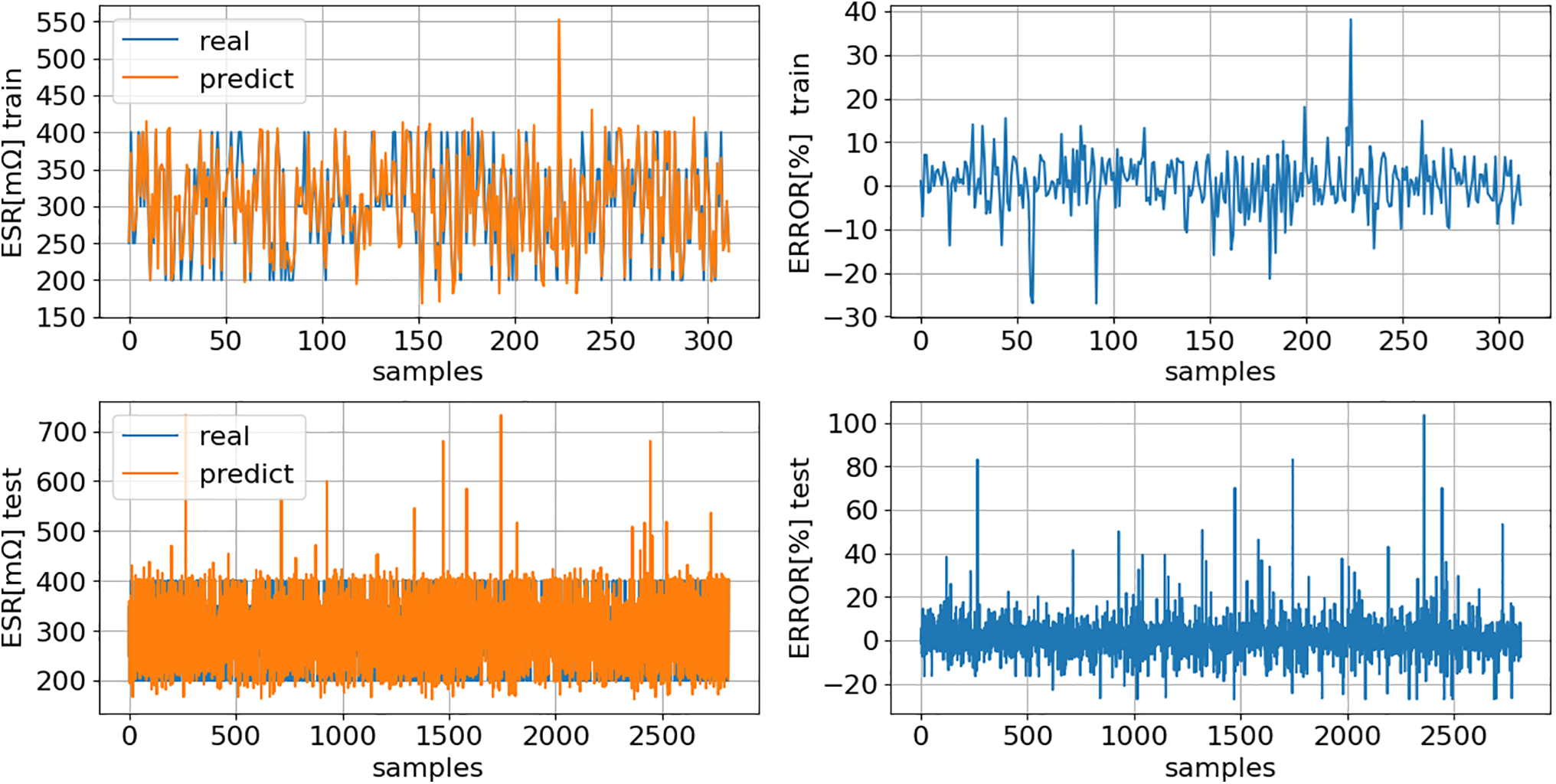
Figure 12: ESR (7): comparison of model predictions (predict) with actual values (real) for both training and testing datasets

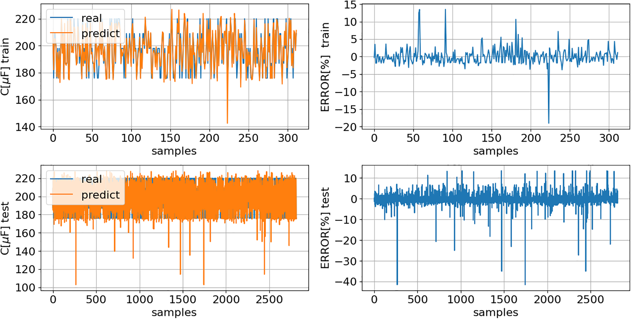
Figure 13: C (8): comparison of model predictions (predict) with actual values (real) for both training and testing datasets

4.2 Comprehensive Model Evaluation and Performance Metrics across All Scenarios

As shown in the procedure presented in the previous section, the cost function used corresponds to the sum of squared errors (SSE) between the model predictions and the actual values, with the objective being to minimize this function to obtain the optimal parameters.

Therefore, the mean squared error (MSE) of the residuals (9) can be used as a metric to evaluate the model’s performance.

{MSEESR=1n×∑i=1n((yi−ESRi(F1,F2,F3,F4,F5,F6))2)MSEC=1n×∑i=1n((yi−Ci(F1,F2,F3,F4,F5,F6))2)(9)

Thus, the MSE value regarding the training dataset (TrDS) was:

∎   MSEESR⌊TrDS≅0.000454

∎   MSEC⌊TrDS≅2.19×10−11

The MSE value regarding the test dataset (TeDS) was:

∎   MSEESR⌊TeDS≅0.000665

∎   MSEC⌊TeDS≅3.22×10−11

As expected, the MSE increased from the TrDS to the TeDS. However, since the increase was small, this suggests that the model generalizes well, especially considering that the TrDS, with samples selected randomly, comprised only 10% of the total samples.

The SSE reflects the variation between the real data and the model predictions, representing the portion of the data that the model fails to explain. In contrast, the total sum of squares (TSS) captures the total variation in the data. To compute TSS, it is assumed that the model is a horizontal line at the mean (y¯) of the real data values. Using SSE and TSS, it is possible to compute another metric, the coefficient of determination, R2, that expresses how much of the total variation is explained by the new model, and can be calculated through (10):

R2=1−SSETSS={RESR2=1−∑i=1n((yi−ESRi(F1,F2,F3,F4,F5,F6))2)∑i=1n((y¯−yi)2)RC2=1−∑i=1n((yi−Ci(F1,F2,F3,F4,F5,F6))2)∑i=1n((y¯−yi)2)(10)

Thus, the R2 value regarding the TrDS was:

∎   R2ESR⌊TrDS≅0.9014

∎   R2C⌊TrDS≅0.9014

The R2 value regarding the TeDS was:

∎   R2ESR⌊TeDS≅0.8680

∎   R2C⌊TeDS≅0.8680

The results above indicate that both models explain 90.14% of the variability in the training data and 86.80% of the variability in the test data. The relatively small performance drop of just 3.70% between the two datasets demonstrates strong generalization and suggests that the model does not exhibit signs of overfitting. Following the model’s performance will be analyzed by severity level.

4.3 Performance Analysis by Severity Level

In order to assess model performance across each severity level, the MSE was first computed for the entire dataset (MSE[AllDS]), followed by separate calculations for each severity level (MSEESR[Si]). Afterwards, the comparison metrics MSE[Diff], that represents the percentage difference between the MSE at a specific severity level (Si) and the entire dataset, was defined as:

MSEESR[Diff]=MSEESR[Si]−MSEESR[AllDS]MSEESR[AllDS]×100%(11)

MSEC[Diff]=MSEC[Si]−MSEC[AllDS]MSEC[AllDS]×100%(12)

Analysis of Figs. 12 and 13 reveals that models (7) and (8) show MSEESR[Diff] and MSEC[Diff] approaching 200% for severity level S4, whereas the other severity levels display negative MSE[Diff] values. This suggests that both models present greater difficulty in estimating the ESR and C values for severity level S4. To confirm the previous results, 200 linear models were trained using Eq. (4), each based on a different TrDS consisting of 10% randomly selected samples from the original dataset (Fig. 7). The models were then evaluated for each of the different severity levels.

Fig. 14 presents the MSEESR[Diff] for the first hundred models (ESR estimation).

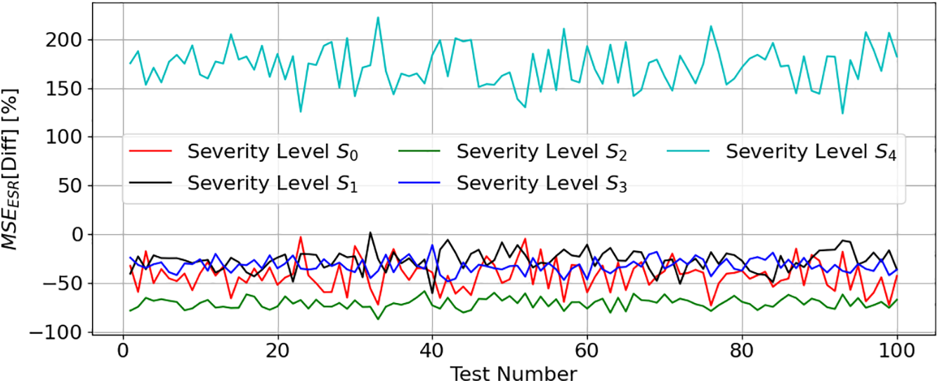
Figure 14: MSEESR[Diff] values by severity level for 100 independently trained models using 10% of samples randomly selected from the original dataset (ESR estimation)

Fig. 15 presents the MSEC[Diff] for the second hundred models (C estimation).

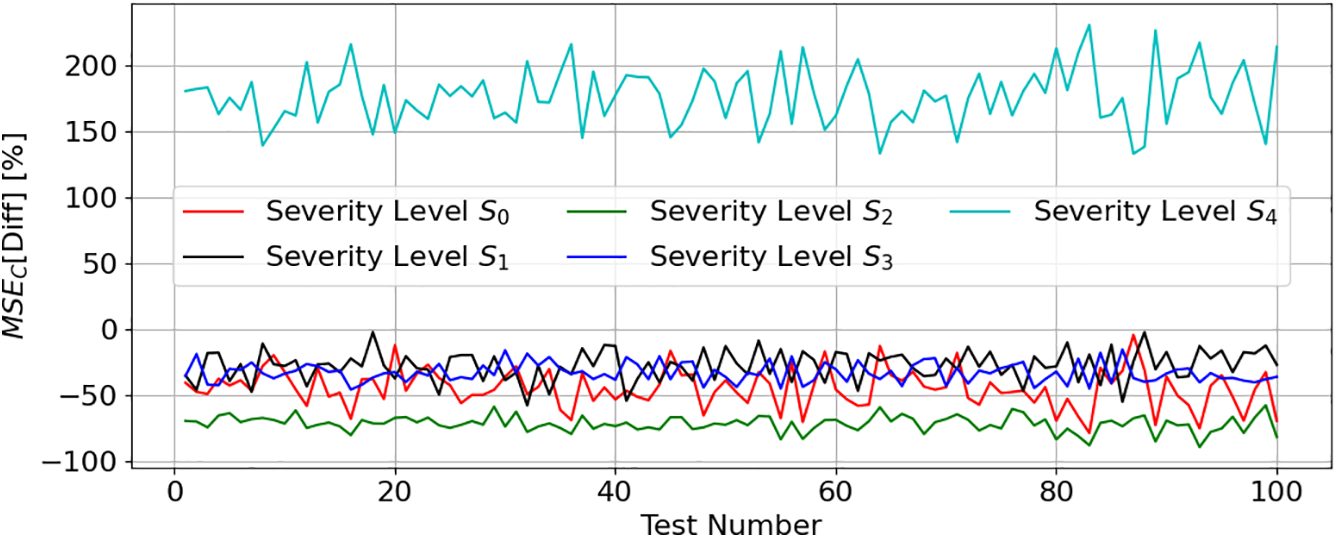
Figure 15: MSEC[Diff] values by severity level for 100 independently trained models using 10% of samples randomly selected from the original dataset (C estimation)

Figs. 14 and 15 confirm the earlier analysis: models represented in (4) demonstrate greater difficulty estimating ESR and C values at severity level S4. This difficulty stems from the nonlinear capacitor impedance (ZC) behavior, which directly affects voutAC feature value.

ZC=ESR2+(12×π×f×C)2(13)

where f represents the frequency.

The nonlinear influence of ZC on the voutAC feature represents a challenge for the linear models (4), resulting in worse performance for severity level S4.

4.4 Performance Evaluation Against Alternative Signal Processing Techniques (SPT)

To evaluate the performance of the proposed technique in comparison with other signal processing techniques (SPT), the approach described in [43] was selected. This new SPT combines a bandpass filter with the Hilbert transform, which is why it will be denominated as the Hilbert approach. Initially, the band-pass filter isolates the spectral component of the signal associated with the frequency of interest, the converter’s switching frequency. Subsequently, the Hilbert transform is applied to extract the envelope of the filtered signal. This process involves two steps: extraction of the signal envelope through the Hilbert transform and filtering of the average amplitudes using a sliding window with a WS of 1000 samples and a HS of 500 samples. These processing steps produce the AC component of the signal, which represents the AC features used as input to the ML algorithm. Further details regarding the implementation of this SPT can be found in [43].

The comparative analysis will contrast the Hilbert approach with the method from Section 2, which combines a bandpass filter with an RMS filter, the latter being denoted as the RMS approach. To perform this comparative analysis, 100 linear regression models were trained for each approach, with 10% of the data allocated to the TrDS and 90% to the TeDS. Samples were randomly selected from the original dataset (ODS). The RMS approach used the ODS presented in Fig. 7, whereas the Hilbert transform approach required generating a new ODS under identical operating conditions (Fig. 2) and severity levels (Fig. 6) as those in Fig. 7. Both methods were evaluated using the R2 score metric, with results displayed in Fig. 16.

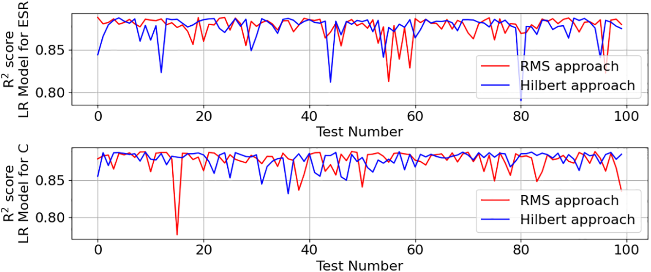
Figure 16: Comparative performance analysis of the proposed solution against SPT: RMS approach vs. Hilbert approach

Both methods demonstrated comparable performance, with average R2 scores of approximately 0.87 for both ESR and C estimations. Consequently, the RMS-based approach was selected for further use.

4.5 Performance Evaluation against Alternative Machine Learning Algorithms

In this section, a comparison will be made between the ML model used, the linear regression (LR), and another ML algorithm, namely the K-Nearest Neighbors (KNN) algorithm.

The KNN algorithm is a nonparametric ML algorithm that stores all observations from the TrDS and uses them to make predictions based on similarity or distance functions, such as Euclidean distance, Manhattan distance, and others [44].

During the inference stage, the K-nearest neighbors of the test data sample for which the prediction is being made are identified, using the stored TrDS. In this step, the distance between the test point (TeDS sample) and each point in the TrDS is calculated, commonly using the Euclidean distance [45], and the K-nearest neighbors are identified. The Euclidean distance between two data points can be computed as follows [46]:

d(X,X′)=(xF1−xF1′)2+…+(xF6−xF6′)2(14)

where X represents a point in TrDS, X′ is the TeDS sample, xFi is the value of the i-th feature of X and xFi′ is the value of the i-th feature of X′.

Once the K-nearest neighbors are identified, and if the weight parameter is set to ‘uniform’, the prediction p of sample xj, p(xj), from TeDS is computed by averaging the target values (y) of the K-nearest points from the TrDS. Therefore, p(xj) can be computed as follows:

p(xj)=1k×∑i=1kyi(15)

Parameter optimization presents a primary challenge in KNN application, specifically determining the optimal number of neighbors (K), selecting the appropriate distance metric, and defining the weighting scheme for nearest neighbors. Thus, these three parameters were tuned based on the values presented in Table 2. The evaluation metric used during the tuning stage was the R2 score.

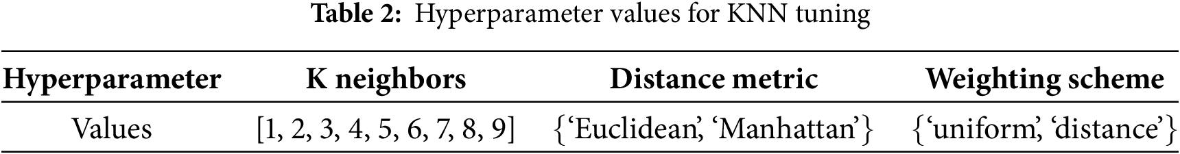
Hence, grid search with cross-validation was applied to a randomly selected 10% subset of the ODS to identify the hyperparameters that optimized model performance: k = 2, distance = ‘Euclidean’, and weighting = ‘distance’. The parameter weights = ‘distance’ indicates that closer neighbors have a greater influence on the prediction than more distant ones.

The KNN algorithm was subsequently applied to the ODS (Fig. 7), using a 10% subset for training with randomly selected samples. The estimation errors for ESR and C parameters are presented in Fig. 17.

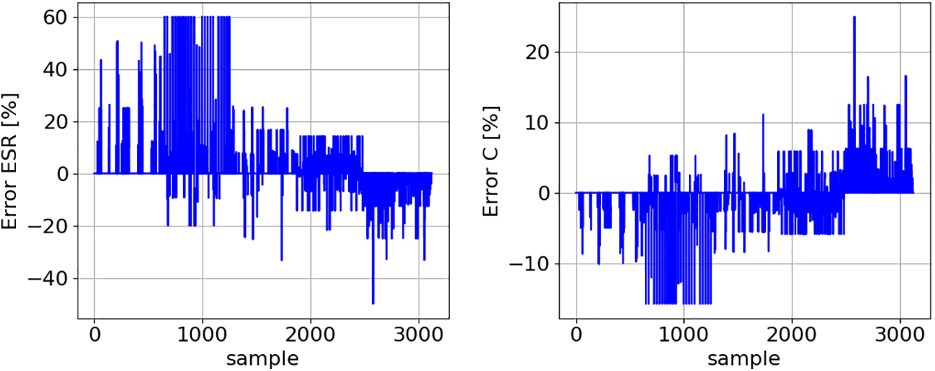
Figure 17: Prediction errors obtained when applying the KNN algorithm to the ODS (Fig. 7)

Fig. 17 demonstrates that KNN has greater difficulty in predicting the ESR and C values for the second severity level (S1). The R2 score is around 0.89, which allows us to conclude that the KNN algorithm slightly outperforms the LR algorithm. However, this approach has significant practical limitations due to its dependence on the TrDS. Thus, substantial memory resources may be required to store the TrDS, which depends not only on the number of samples but also on the number of features. This memory requirement poses considerable challenges for implementing this solution on microcontrollers.

5  Model Training and Evaluation—Feature Engineering

Although the linear regression model presented in the previous section performed well, this section explores the creation of new features to further improve the model’s performance. These new features will be derived from existing ones through transformations, as part of the feature engineering process.

The new features are generated through polynomial transformations of the existing features. For example, given two features, x1 and x2, the transformation produces additional features such as x12, x22 and (x1 × x2). This approach could account for the nonlinear relationships outlined in Section 4.3.

Accordingly, the new features were created taking into account the original features. Therefore, regarding the original ones, there are six:

∎   iinAC, iinDC, ioutAC, voutAC, voutDC and R;

Regarding the new features, there are twenty-one:

∎   The new features are: iinAC2, iin_AC × iinDC, iinAC × ioutAC, iinAC × voutAC, iinAC × voutDC, iinAC × R, iinDC2, iinDC × ioutAC, iinDC × voutAC, iinDC × voutDC, iinDC × R, ioutAC2, ioutAC × voutAC, ioutAC × voutDC, ioutAC × R, voutAC2, voutAC × voutDC, voutAC × R, vout_DC2, voutDC × R and R2.

As the number of features increased from 6 to 27, cross-validation was used to evaluate the model’s ability to generalize to unseen data.

Initially, the dataset, containing 27 features, was divided into a training set (TrDS) comprising 25% of the total randomly selected samples and a test set (TeDS) comprising the remaining 75% of the samples. However, to better evaluate the performance of the linear models used to estimate both ESR and C, cross-validation was employed to assess their ability to generalize. Hence, the TrDS was then split into 10 equal-sized folders. The models were trained and evaluated 10 times, with a different folder being used for testing and the remaining nine for training in each iteration. This ensures that each data sample is used once for testing and nine times for training. Table 3 presents the R2 scores obtained across the 10 cross-validation iterations for both models: ESR(F1,…,F27) and C(F1,…,F27).

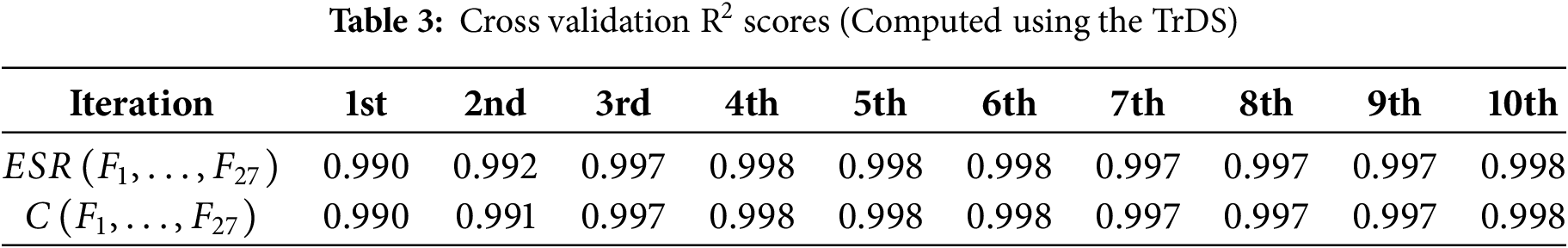
Since the R2 values are consistent across the 10 iterations, this suggests that the models generalize well and are unlikely to overfit in the TrDS.

Once the models’ generalization capabilities were confirmed, both were trained on the TrDS, resulting in the following mathematical models for ESR(F1,…,F27) and C(F1,…,F27):

ESR(F1,…,F27)=8.76×iinAC−26.93×iinDC−1.60×ioutAC+3.28×voutAC−3.21×voutDC−0.46×R−0.53×iinAC2+1.11×iinAC×iinDC−0.15×iinAC×ioutAC−0.24×iinAC×voutAC−1.20×iinAC×voutDC−0.58×iinAC×R+1.74×iinDC2+0.17×iinDC×ioutAC+7.77×iinDC×voutAC+33.81×iinDC×voutDC+31.20×iinDC×R+0.38×ioutAC2+0.26×ioutAC×voutAC−4.81×ioutAC×voutDC−5.15×ioutAC×R−0.10×voutAC2−0.22×voutAC×voutDC−0.12×voutAC×R−7.49×voutDC2−0.06×voutDC×R+0.03×R2+0.475(16)

C(F1,…,F27)=−1.93×10−3×iinAC+5.93×10−3×iinDC+3.52×10−4×ioutAC−7.22×10−4×voutAC+7.06×10−4×voutDC+1.00×10−4×R+1.16×10−4×iinAC2−2.44×10−4×iinAC×iinDC+3.31×10−5×iinAC×ioutAC+5.21×10−5×iinAC×voutAC+2.64×10−4×iinAC×voutDC+1.28×10−4×iinAC×R−3.83×10−4×iinDC2−3.71×10−5×iinDC×ioutAC−1.71×10−3×iinDC×voutAC−7.44×10−3×iinDC×voutDC−6.87×10−3×iinDC×R−8.30×10−5×ioutAC2−5.73×10−5×ioutAC×voutAC+1.06×10−3×ioutAC×voutDC+1.13×10−3×ioutAC×R+2.27×10−5×voutAC2+4.94×10−5×voutAC×voutDC+2.57×10−5×voutAC×R+1.65×10−3×voutDC2+1.40×10−5×voutDC×R−5.77×10−6×R2+0.000159(17)

Figs. 18 and 19 provide a comparison between the ESR(F1,…,F27) and C(F1,…,F27) models predictions and the actual values, both for the TrDS and the TeDS. It’s important to highlight that the TeDS data has never been seen by the models before.

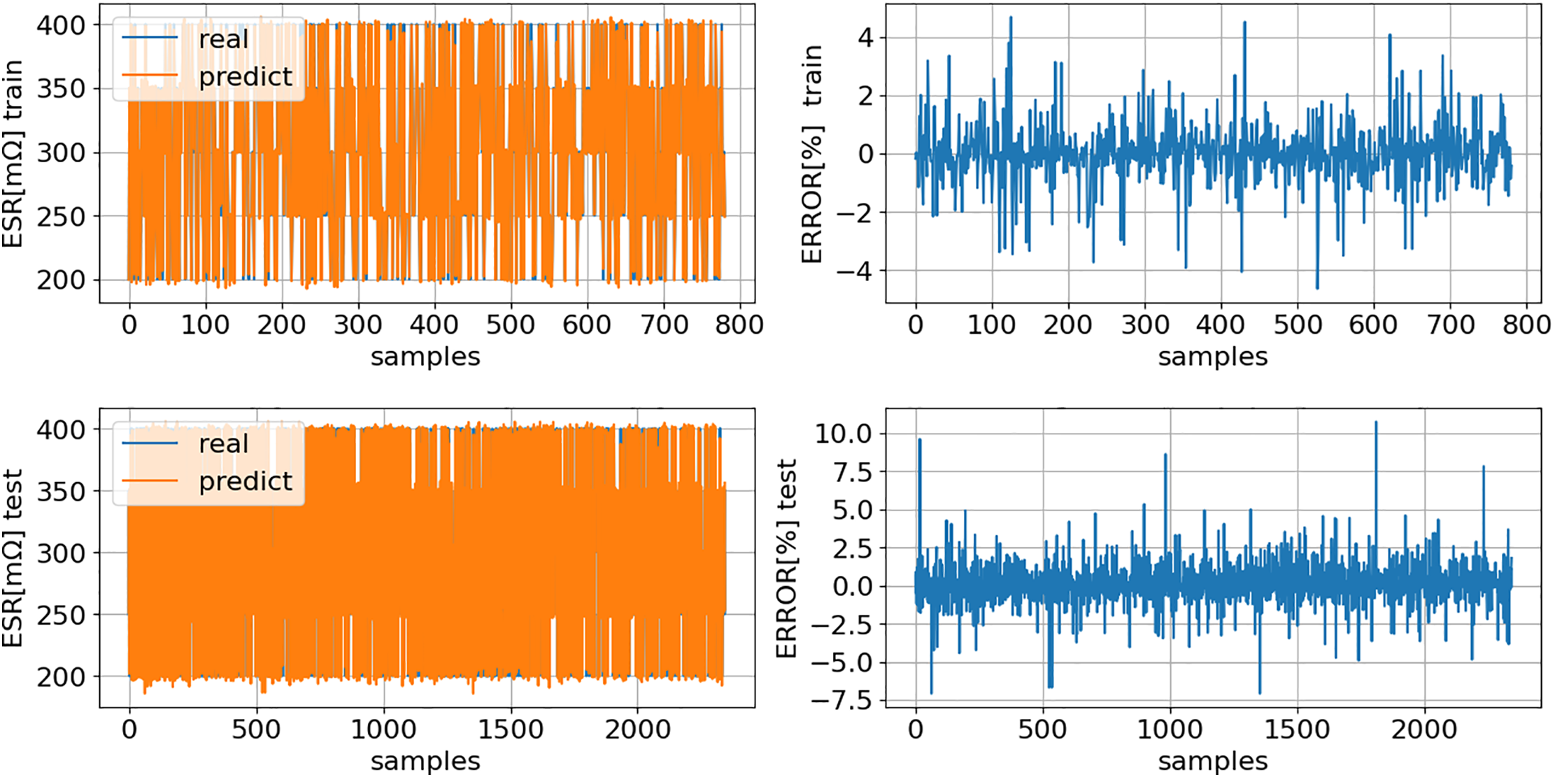
Figure 18: ESR (16): comparison of model predictions (predict) with actual values (real) for both training (TrDS) and testing (TeDS) datasets

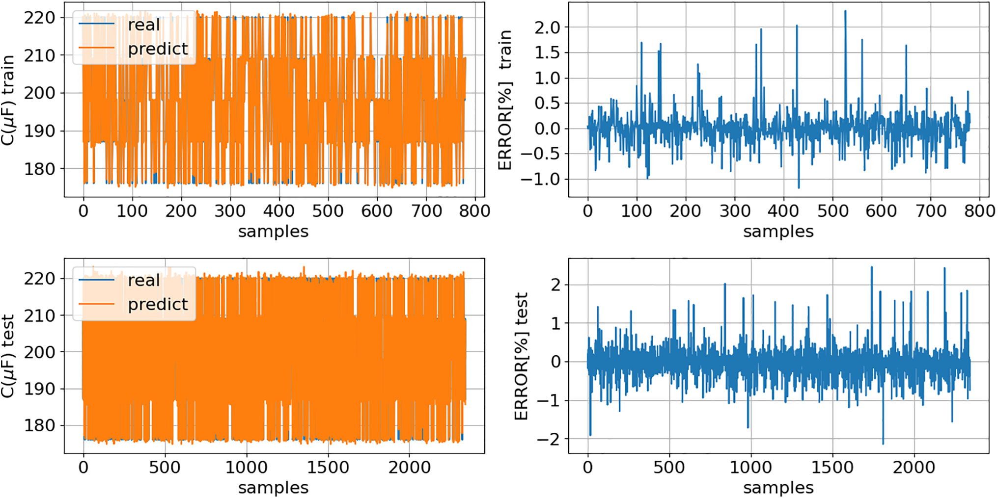
Figure 19: C (17): comparison of model predictions (predict) with actual values (real) for both training (TrDS) and testing (TeDS) datasets

Figs. 18 and 19 demonstrate that the models (16) and (17) outperform the models (7) and (8), with the R2 score improving in the test dataset from 0.87 to 0.99. Figs. 20 and 21 show the prediction of models (16) and (17), respectively, for the entire dataset (Fig. 7). It is important to note that 75% of the data presented in the following two figures represents previously unseen data.

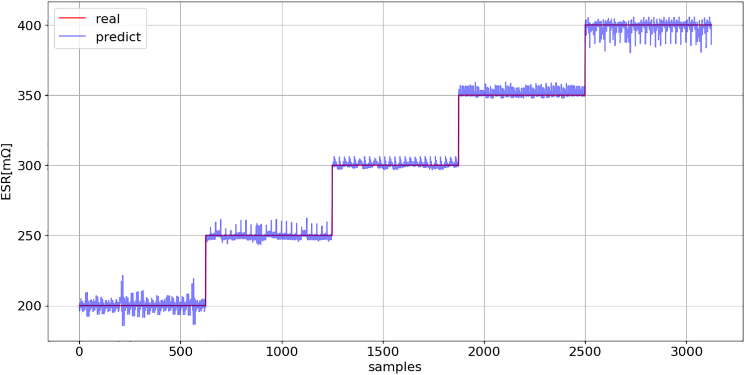
Figure 20: ESR prediction (16): comparison between model predictions and actual values across the entire dataset

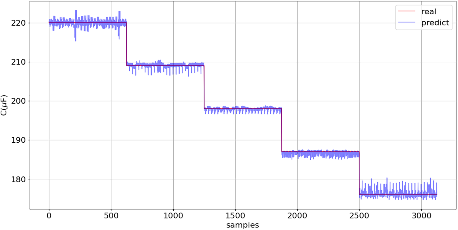
Figure 21: C prediction (17): comparison between model predictions and actual values across the entire dataset

Figs. 20 and 21 corroborate the previous conclusion, clearly demonstrating that models (16) and (17) enable accurate estimation of ESR and C values, respectively.

The models were then evaluated by severity level, showing a slight decline in accuracy when estimating ESR and C values at the highest severity level (S4). However, with MSE[Diff] values remaining below 63%. This suggests that, despite the reduced performance at S4, models (16) and (17) still outperform models (7) and (8) in estimating ESR and C at this severity level relative to the other severity levels. These findings suggest that models (16) and (17) provide improved representations of nonlinear behavior, enabling them to better address the effect described in Section 4.3. Although enhanced performance could be achieved through increased model complexity, the current 27-features configuration represents a trade-off between accuracy and computational efficiency for microcontroller implementation.

The KNN algorithm was also implemented using all 27 features. Following hyperparameter optimization, the configuration yielding the better KNN performance consisted of k = 3, distance = ‘Manhattan’ and weighting = ‘distance’.

Fig. 22 displays the prediction results of the KNN models for both ESR and C.

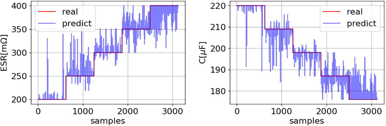
Figure 22: ESR and C prediction using the KNN model: comparison between model predictions and actual values across the entire dataset

Fig. 22 demonstrates that the KNN models perform worse than the models (16) and (17), as confirmed by their R2 score of 0.97.

The following section will discuss the implementation or deployment phase of the model.

6  Deployment Phase

The model’s implementation or deployment phase involves applying it to an entirely new, unseen dataset. Accordingly, a new dataset was created comprising 225 distinct operating conditions (Fig. 23) and six new severity levels (Fig. 24), resulting in a total of 225 × 6 = 1350 samples (Fig. 25).

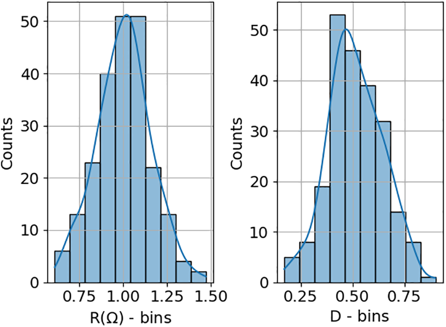
Figure 23: Range of randomly defined operating conditions, regarding a new dataset consisting of 225 distinct operating conditions, where R denotes the load resistance and D the duty cycle

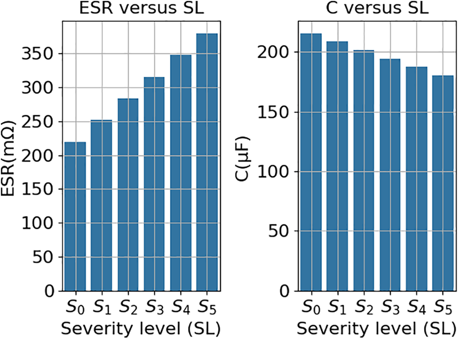
Figure 24: Severity levels included in the new dataset

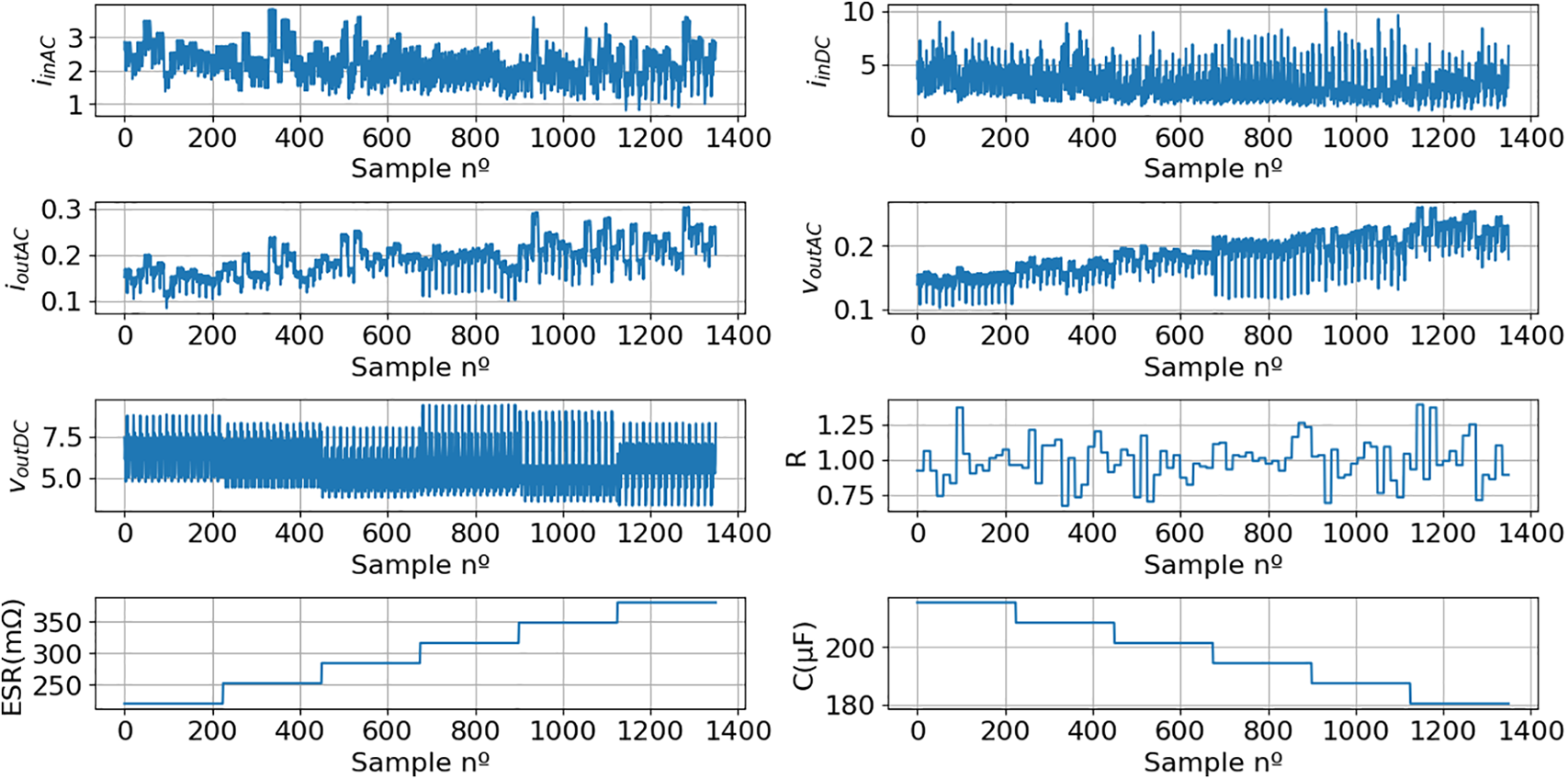
Figure 25: The new dataset, derived from 1350 simulations, containing the primary features (iinAC, iinDC, ioutAC, voutAC, voutDC and R) and target variables (ESR and C)

To assess the model’s generalization capability, significantly different severity levels beyond those used in the training and evaluation phases were selected for the deployment phase. The training and evaluation phases used just 5 severity levels (ESR = {200, 250, 300, 350, 400} mΩ and C = {220, 209, 198, 187, 176} μF), whereas the deployment phase incorporated 6 severity levels (ESR = {220, 252, 284, 316, 348, 380} mΩ and C = {215.6, 208.56, 201.52, 194.48, 187.44, 180.4} μF).

6.1 Performance Analysis on an Entirely New Data Set

Subsequently, models (16) and (17) were employed to estimate the ESR and C values on a completely new data set (Fig. 25). Figs. 26 and 27 present a comparison between the predicted and actual values.

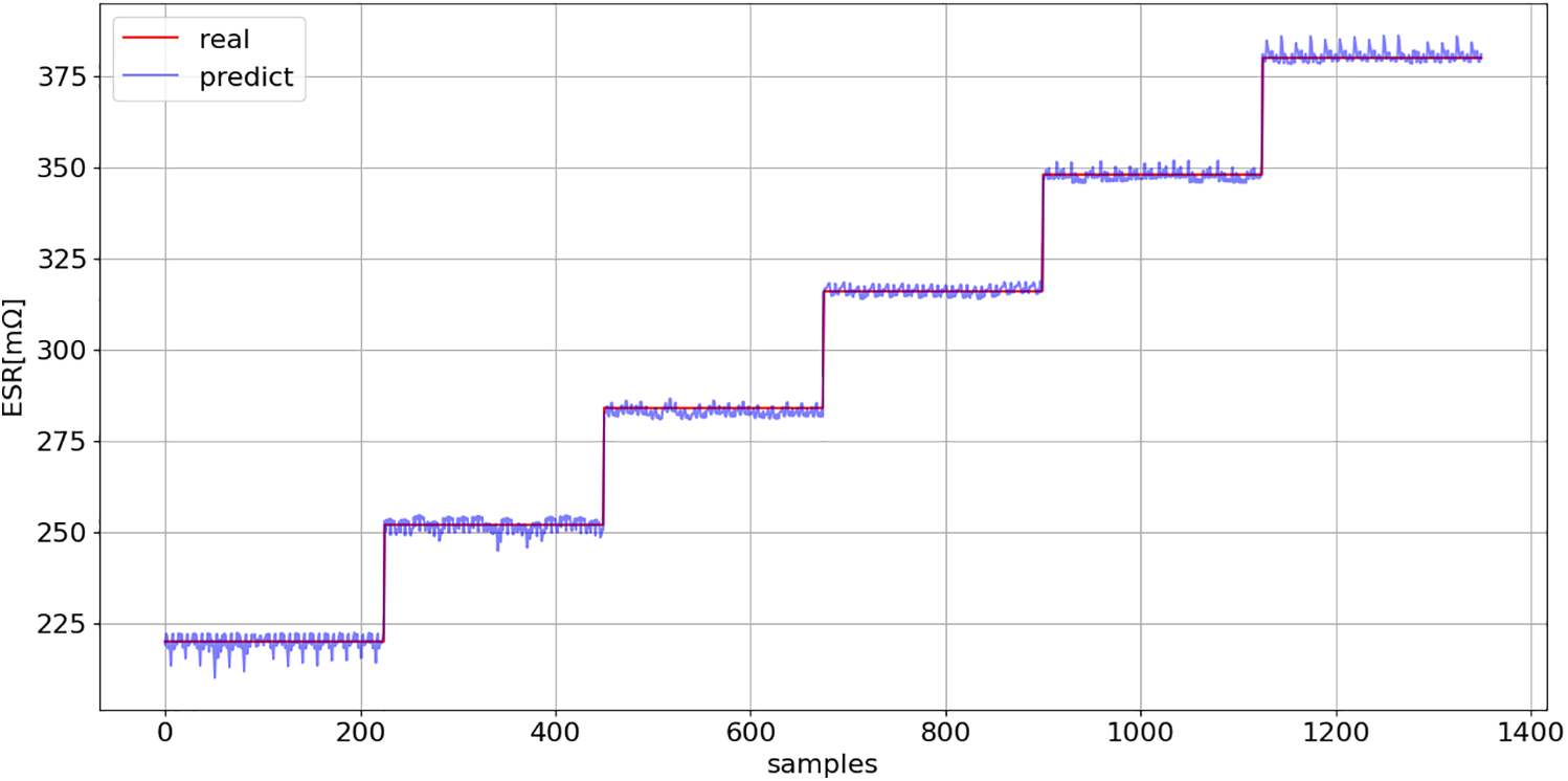
Figure 26: ESR prediction (16): comparison between model predictions and actual values across the entire new dataset (Fig. 25)

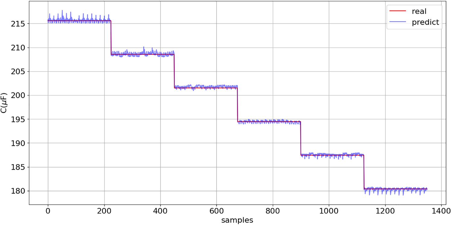
Figure 27: C prediction (17): comparison between model predictions and actual values across the entire new dataset (Fig. 25)

The coefficient of determination of models (16) and (17), on the new dataset (Fig. 25), exceeds 0.99, confirming the model’s excellent generalization capability.

6.2 Model Performance under Progressive Capacitor Aging

This section demonstrates the application of FDT during buck converter operation, with the main electrical specifications of the converter detailed in Table 4. During converter operation, the ESR and C values of the AEC were systematically varied from their nominal conditions (sound AEC) to the critical degradation level, which requires AEC replacement.

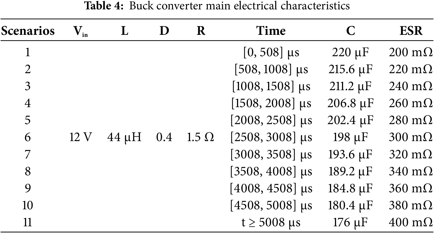
Fig. 28 presents a comparison between the ESR and C value predictions from models (16) and (17) and their corresponding actual measurements for the buck converter operating under the conditions specified in Table 4.

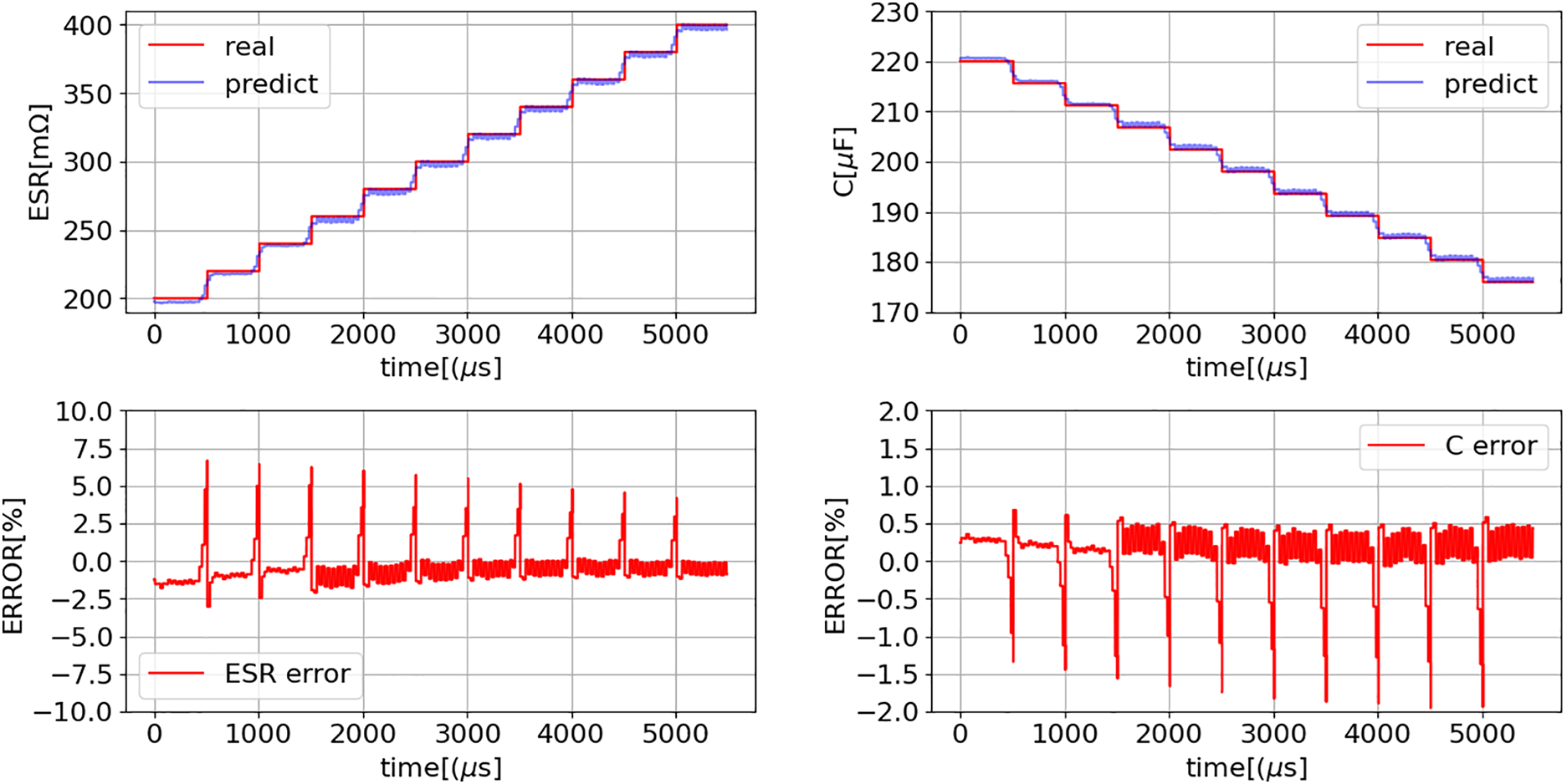
Figure 28: Comparison of estimated ESR and C from Eqs. (16) and (17) with the actual values for the buck converter operating under the conditions specified in Table 4

Fig. 28 illustrates the application of models (16) and (17) during buck converter operation under the conditions specified in Table 4. In all eleven cases, the estimation errors for ESR and C were below 10% and 2%, respectively, demonstrating that the models can effectively assess the condition of the AECs during converter operation without requiring additional sensors or complex computations.

6.3 Assessment of Model Robustness to Environmental Noise

To assess the impact of noise, a noise component was added to the input signals (iin, iout, and vout) for the 11 scenarios described in Table 4. The noise sensitivity evaluation employed input signals characterized by a signal-to-noise ratio (SNR) of less than 30 dB, as shown in Fig. 29.

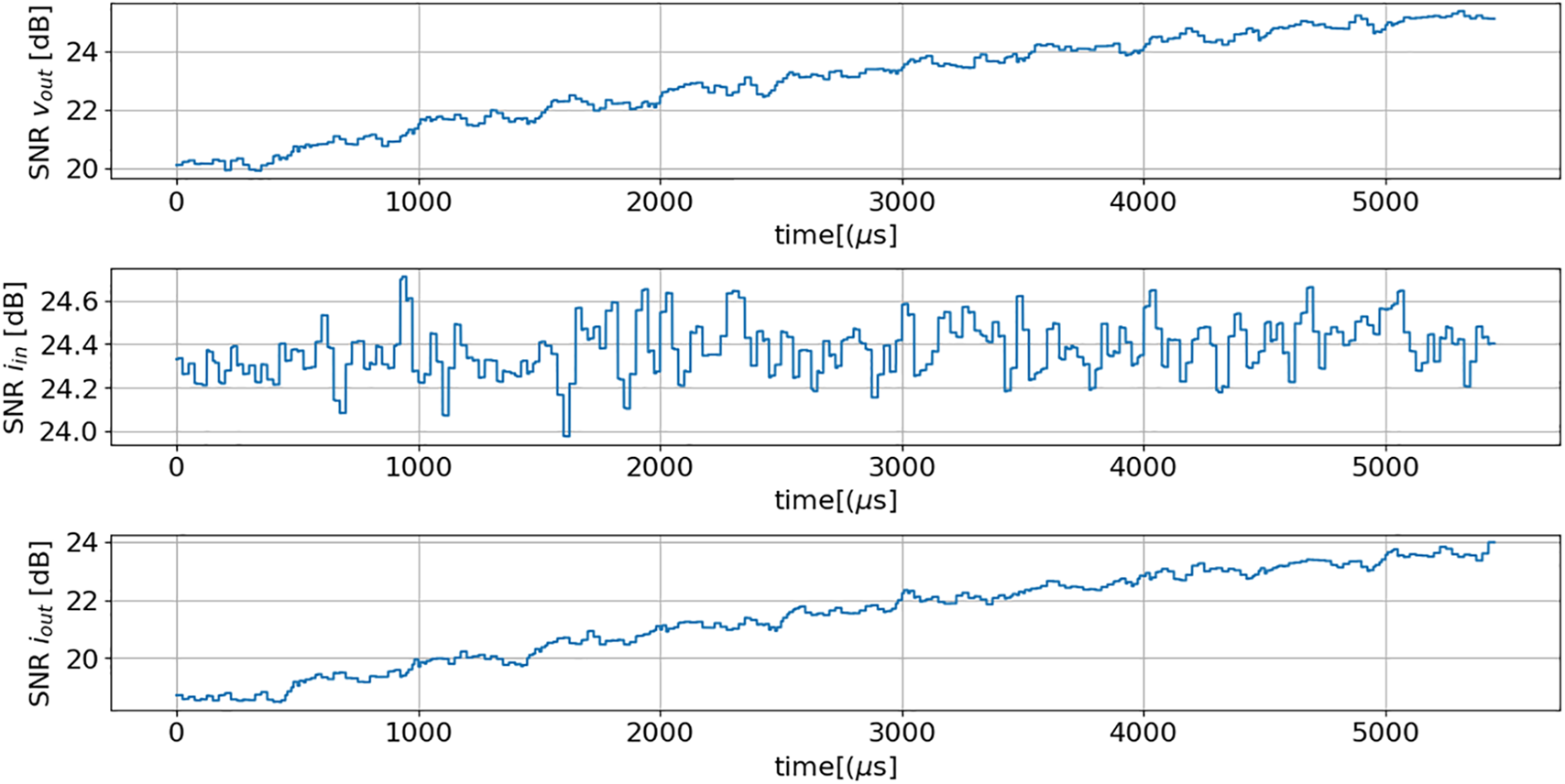
Figure 29: Signal-to-noise ratios (SNR) of input signals, regarding the scenarios described in Table 4, for testing the noise robustness of models (16) and (17)

The responses of models (16) and (17), accounting for the effect of noise, are presented below (Fig. 30).

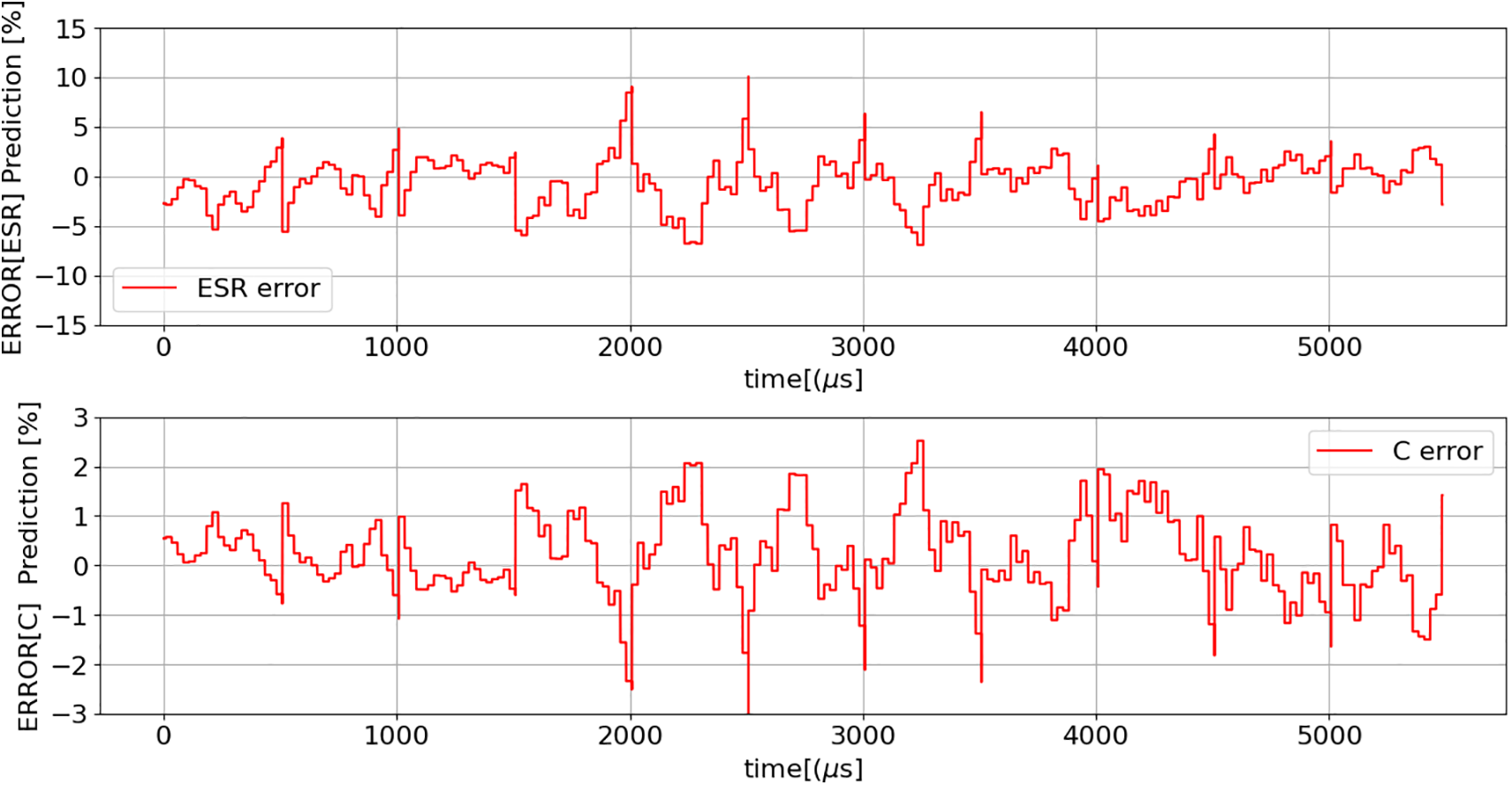
Figure 30: Estimation errors of ESR and C values using models (16) and (17), for the scenarios described in Table 4, considering the presence of noise (as shown in Fig. 29)

The previous figure clearly demonstrates that noise has minimal impact on model performance. The ESR estimation error remains below 10%, while the maximum error in estimating C increases only slightly, from 2% to 3%.

7  Scalability of the Proposed Solution

To evaluate the scalability of the proposed solution, it was implemented in a different converter topology (boost converter). This required adapting the approach presented in [42] to enable simulation of the boost converter topology in Python, which was subsequently validated using LTspice. Following, the same procedure applied to the buck converter was then executed. Therefore, a new dataset was generated, comprising 400 distinct operating conditions (Fig. 31) and five additional severity levels (Fig. 6), resulting in a total of 400 × 5 = 2000 samples (Fig. 32).

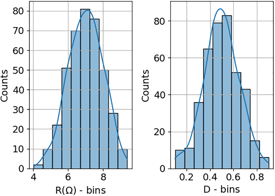
Figure 31: Range of randomly defined operating conditions, regarding the boost converter dataset consisting of 400 distinct operating conditions, where R denotes the load resistance and D the duty cycle. The values of vin (5 V) and L (44 μH) are kept constant throughout all simulations

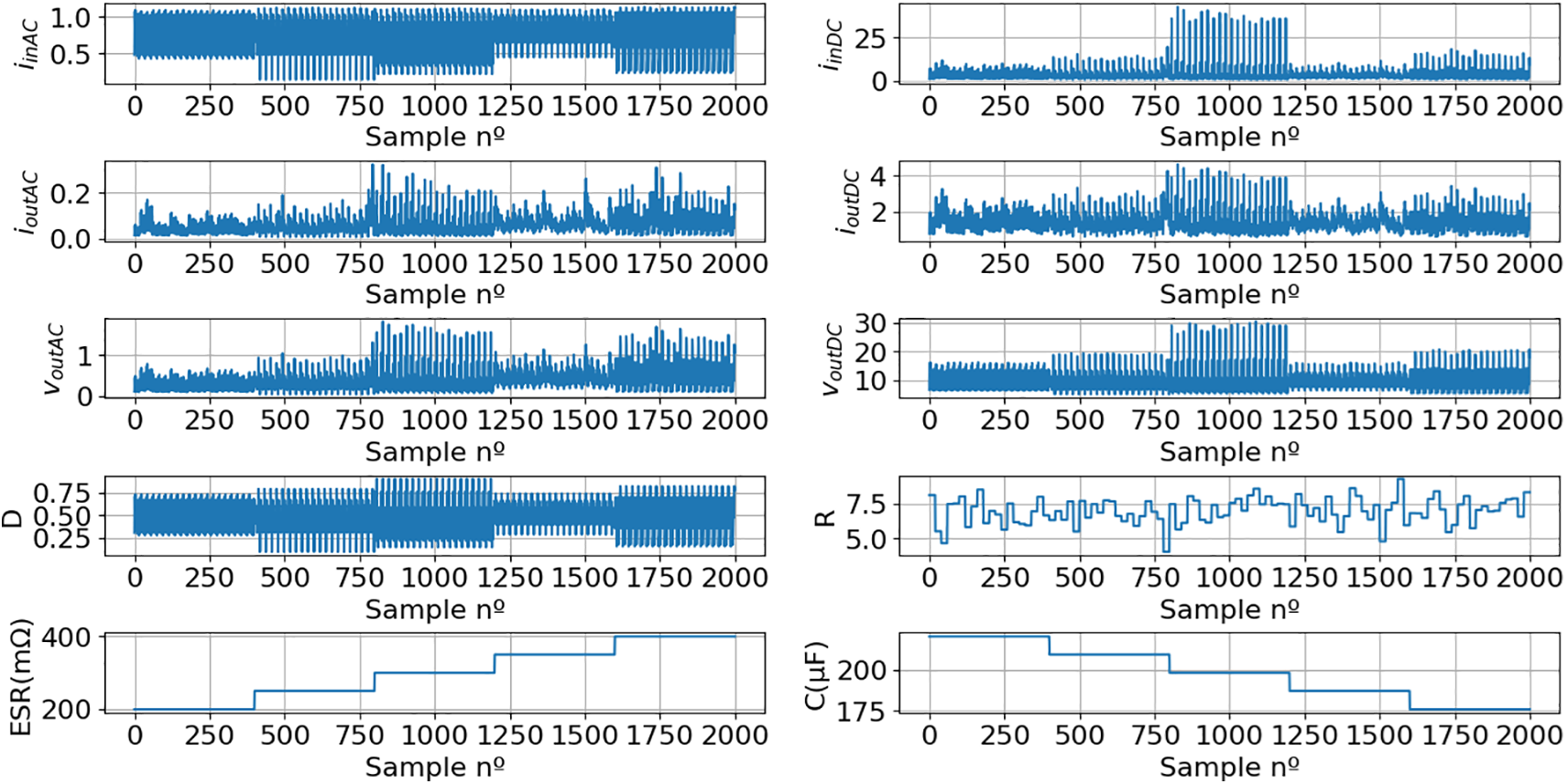
Figure 32: Boost converter dataset, derived from 2000 simulations, containing the primary features (iinAC, iinDC, ioutAC, voutAC, voutDC, and R) and target variables (ESR and C)

A training dataset (TrDS) was then created by randomly selecting 25% of the total samples from the original dataset (Fig. 32).

After completing the training phase, the resulting models for ESR (18) and C (19) were obtained. The parameters for these models are listed in Table 5.

Subsequently, models (18) and (19) were applied to the full original dataset (Fig. 32) to assess their performance and evaluate the potential profitability of using the proposed solution in a boost converter (Figs. 33 and 34).

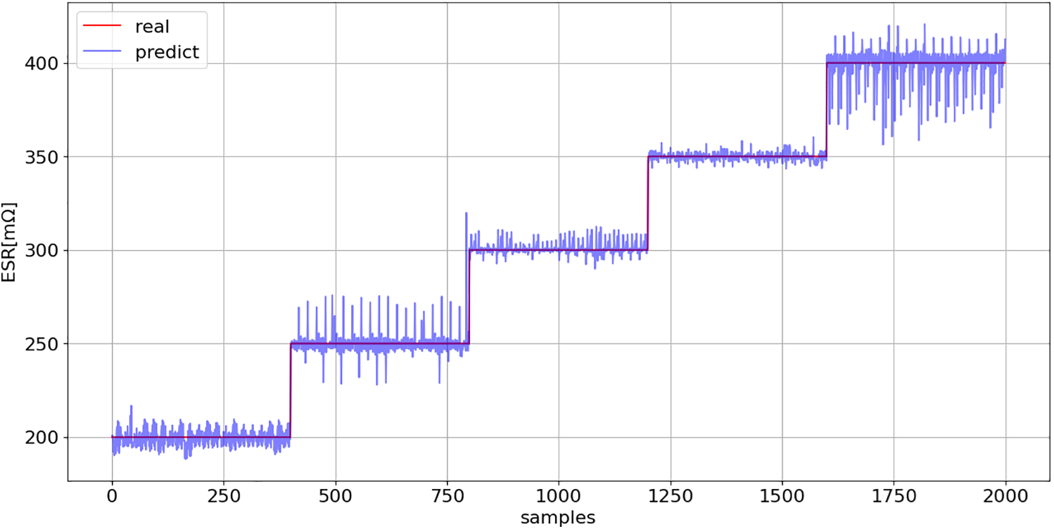
Figure 33: ESR prediction (18): comparison between model predictions and actual values across the entire boost converter dataset (Fig. 32)

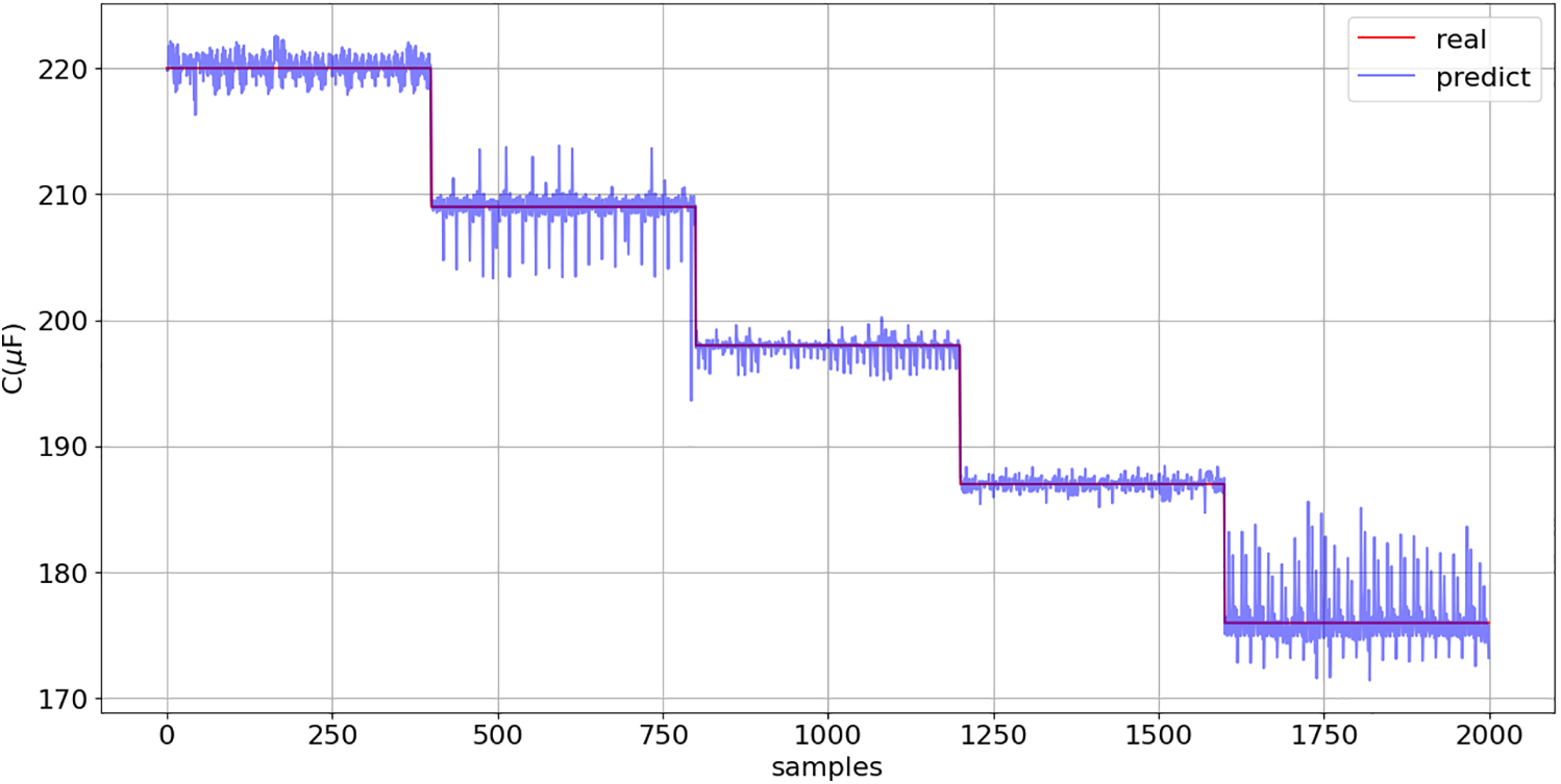
Figure 34: C prediction (19): comparison between model predictions and actual values across the entire boost converter dataset (Fig. 32)

ESR(F1,…,F27)=k0′×iinAC+k1′×iinDC+k2′×ioutAC+k3′×voutAC+k4′×voutDC+k5′×R+k6′×iinAC2+k7′×iinAC×iinDC+k8′×iinAC×ioutAC+k9′×iinAC×voutAC+k10′×iinAC×voutDC+k11′×iinAC×R+k12′×iinDC2+k13′×iinDC×ioutAC+k14′×iinDC×voutAC+k15′×iinDC×voutDC+k16′×iinDC×R+k17′×ioutAC2+k18′×ioutAC×voutAC+k19′×ioutAC×voutDC+k20′×ioutAC×R+k21′×voutAC2+k22′×voutAC×voutDC+k23′×voutAC×R+k24′×voutDC2+k25′×voutDC×R+k26′×R2+bias′(18)

C⁡(F1,…,F27)=k0′′×iinAC+k1′′×iinDC+k2′′×ioutAC+k3′′×VoutAC+k4′′×VoutDC+k5′′×R+k6′′×iinAC2+k7′′×iinAC×iinDC+k8′′×iinAC×ioutAC+k9′′×iinAC×VoutAC+k10′′×iinAC×VoutDC+k11′′×iinAC×R+k12′′×iinDC2+k13′′×iinDC×ioutAC+k14′′×iinDC×VoutAC+k15′′×iinDC×vo⁢u⁢t⁢D⁢C+k16′′×iinDC×R+k17′′×ioutAC2+k18′′×ioutAC×VoutAC+k19′′×ioutAC×VoutDC+k20′′×ioutAC×R+k21′′×VoutAC2+k22′′×VoutAC×VoutDC+k23′′×VoutAC×R+k24′′×VoutAC2+k25′′×VoutDC×R+k26′′×R2+bias′′(19)

The coefficient of determination of models (18) and (19) was greater than 0.994 on the TrDS, which comprised 25% of the original dataset (Fig. 32). The R2 value decreased slightly to 0.991 on the test dataset, which was composed of previously unseen data. These results indicate that the proposed solution possesses excellent generalization capability.

The buck converter generates a DC output voltage lower than the DC input voltage, producing high input current ripple. In contrast, the boost converter provides a DC output voltage higher than the DC input voltage, and the input current ripple is reduced. Despite these topological and operational differences, the proposed solution exhibits robust performance, achieving high coefficients of determination for both converters (greater than 0.99), even on data that has never been seen by the models before. This underscores the high scalability and generalization capability of the proposed solution. Besides, following the model training stage, the full implementation pipeline requires minimal computational resources and can be efficiently implemented on a microcontroller.

8  Conclusions

Power converters are fundamental elements of several critical systems; therefore, failures in these converters can lead to serious safety problems. On the other hand, operational interruptions in these converters can lead to significant financial losses.

One of the most critical elements of power converters are the capacitors used in the output filter, which are responsible for more than 25% of failures. The aging of these components is a gradual process, resulting in increased internal resistance (ESR) and a decrease in capacitance (C) over time. There is a limit to ESR and C beyond which the probability of this failure resulting in catastrophic failure increases significantly; therefore, it is essential to estimate both ESR and C values accurately.

One of the problems associated with estimating ESR and C is the need to introduce sensors inside the converter. The fault diagnosis technique (FDT) proposed in this paper overcomes this problem by using only the input and output waveforms of the converter. Using signal processing and linear regression algorithms, it was possible to produce two models capable of estimating the ESR and C value of capacitors. The FDT is therefore based on estimating the ESR and C values, and when these values exceed the thresholds, replacement of the capacitors must be considered.

The first proposed solution employs a linear regression model that utilizes 6 attributes directly derived from the input and output signals, yielding an R2 score of over 86%. In the second solution, 21 new features are created using feature engineering. This second solution outperforms the first, achieving an R2 score greater than 99%.

In order to validate not only the generalization capability but also the scalability of the proposed solution, it was applied to two distinct converter topologies: a buck converter and a boost converter. In both cases, the models achieved an R2 score greater than 99%, demonstrating an excellent performance. Furthermore, following the training phase, the solution can be efficiently deployed on a microcontroller, as the entire implementation pipeline requires minimal computational resources.

In summary, the proposed solution is well-suited for implementation on a microcontroller, as it requires minimal computational resources, avoids the need for internal sensors within the converter, and demonstrates strong generalization capability and scalability.

Acknowledgement: Not applicable.

Funding Statement: The author received no specific funding for this study.

Availability of Data and Materials: Not applicable.

Ethics Approval: Not applicable.

Conflicts of Interest: The author declares no conflicts of interest to report regarding the present study.

References

1. Energy statistics—an overview [Internet]. Luxembourg: Eurostat; [cited 2025 Aug 3]. Available from: https://ec.europa.eu/eurostat/statistics-explained/index.php?title=Energy_statistics_-_an_overview. [Google Scholar]

2. Electricity 2024—analysis and forecast to 2026 [Internet]. Paris, France: IEA Publications; [cited 2025 Aug 3]. Available from: https://www.iea.org/reports/electricity-2024. [Google Scholar]

3. Scolaro E, Beligoj M, Estevez MP, Alberti L, Renzi M, Mattetti M. Electrification of agricultural machinery: a review. IEEE Access. 2021;9:164520–41. doi:10.1109/access.2021.3135037. [Google Scholar] [CrossRef]

4. Ahmed B, Shabbir H, Naqvi SR, Peng L. Smart agriculture: current state, opportunities, and challenges. IEEE Access. 2024;12(1):144456–78. doi:10.1109/access.2024.3471647. [Google Scholar] [CrossRef]

5. Meng L, Hirayama T, Oyanagi S. Underwater-drone with panoramic camera for automatic fish recognition based on deep learning. IEEE Access. 2018;6:17880–6. doi:10.1109/access.2018.2820326. [Google Scholar] [CrossRef]

6. Pate K, El Breidi F, Salem T, Lumkes J. Industry perspectives on electrifying heavy equipment: trends, challenges, and opportunities. Energies. 2025;18(11):2806. doi:10.3390/en18112806. [Google Scholar] [CrossRef]

7. Torcato JC, Silva R, Eusébio M. Electrification of compressor in steam cracker plant: a path to reduced emissions and optimized energy integration. ChemEngineering. 2025;9(3):55. doi:10.3390/chemengineering9030055. [Google Scholar] [CrossRef]

8. Borgosano S, Martini D, Longo M, Foiadelli F. Electrifying urban transportation: a comparative study of battery swap stations and charging infrastructure for taxis in Chicago. IEEE Access. 2024;12(1):48017–26. doi:10.1109/access.2024.3379138. [Google Scholar] [CrossRef]

9. Silva CGDS, Peres LAP. Introducing electric bus fleets in Rio de Janeiro City methodology and analysis. IEEE Lat Am Trans. 2022;20(8):2087–95. doi:10.1109/tla.2022.9853229. [Google Scholar] [CrossRef]

10. Yang G, Ye Z, Wu H, Li C, Wang R, Kong D, et al. A digital twin-based large-area robot skin system for safer human-centered healthcare robots toward healthcare 4.0. IEEE Trans Med Robot Bionics. 2024;6(3):1104–15. doi:10.1109/TMRB.2024.3421635. [Google Scholar] [CrossRef]

11. Ma BJ, Kuo YH, Jiang Y, Huang GQ. RubikCell: toward robotic cellular warehousing systems for e-commerce logistics. IEEE Trans Eng Manag. 2023;71:9270–85. doi:10.1109/TEM.2023.3327069. [Google Scholar] [CrossRef]

12. Cardoso AJM. Diagnosis and fault tolerance of electrical machines, power electronics and drives. Stevenage, UK: The Institution of Engineering and Technology; 2018. [Google Scholar]

13. Park HM, Lee HW, Park CB, Lee JB, Kim JC, Lee J. Analysis and design of a 50-kW two stage converters for EV fast charger with high efficiency and wide output voltage of 150–1000 V. IEEE Access. 2025;13:37182–97. doi:10.1109/access.2025.3544277. [Google Scholar] [CrossRef]

14. Geng J, Mandrioli R, Jiang CQ, Ricco M. Vertically stacked dual-bus DC-DC converter for data center high-current power delivery. IEEE Trans Power Electron. 2025;40(5):7002–14. doi:10.1109/TPEL.2025.3532833. [Google Scholar] [CrossRef]

15. Seyezhai R, Maheswari E. Analysis and realization of a Manitoba converter for portable medical devices. In: Proceedings of the 2023 International Conference on Innovative Computing, Intelligent Communication and Smart Electrical Systems (ICSES); 2023 Dec 14–15; Chennai, India. p. 1–6. doi:10.1109/ICSES60034.2023.10465407. [Google Scholar] [CrossRef]

16. Corporation N. General descriptions of aluminum electrolytic capacitors—technical notes cat.8101e-1 [Internet]. [cited 2025 Aug 3]. Available from: https://www.nichicon.co.jp/english/products/pdf/aluminum-e.pdf. [Google Scholar]

17. Panasonic Industry. Technical guide: aluminum electrolytic capacitor, conductive polymer hybrid aluminum and electrolytic capacitor. Osaka, Japan: Panasonic Industry; 2024. [Google Scholar]

18. Dubilier C. Aluminum electrolytic capacitor application guide1 [Internet]. [cited 2025 Aug 3]. Available from: https://www.cde.com/resources/technical-papers/AEappGuide.pdf. [Google Scholar]

19. Amaral AMR, Laadjal K, Marques Cardoso AJ. Advancements in fault diagnosis techniques for aluminium capacitors using STLSP and autoencoder. In: Proceedings of the 2024 IEEE International Conference on Artificial Intelligence & Green Energy (ICAIGE); 2024 Oct 10–12; Yasmine Hammamet, Tunisia. p. 1–6. doi:10.1109/ICAIGE62696.2024.10776613. [Google Scholar] [CrossRef]

20. Agarwal N, Ahmad MW, Anand S. Quasi-online technique for health monitoring of capacitor in single-phase solar inverter. IEEE Trans Power Electron. 2018;33(6):5283–91. doi:10.1109/TPEL.2017.2736162. [Google Scholar] [CrossRef]

21. Gao Z, Cecati C, Ding SX. A survey of fault diagnosis and fault-tolerant techniques: part I: fault diagnosis with model-based and signal-based approaches. IEEE Trans Ind Electron. 2015;62(6):3757–67. doi:10.1109/TIE.2015.2417501. [Google Scholar] [CrossRef]

22. Amaral AMR, Laadjal K, Marques Cardoso AJ. Optimized preventive diagnostic algorithm for assessing aluminum electrolytic capacitor condition using discrete wavelet transform and Kalman filter. Electronics. 2024;13(16):3265. doi:10.3390/electronics13163265. [Google Scholar] [CrossRef]

23. Kumar GK, Elangovan D. Review on fault-diagnosis and fault-tolerance for DC-DC converters. IET Power Electron. 2020;13(1):1–13. doi:10.1049/iet-pel.2019.0672. [Google Scholar] [CrossRef]

24. Rahimpour S, Husev O, Vinnikov D, Kurdkandi NV, Tarzamni H. Fault management techniques to enhance the reliability of power electronic converters: an overview. IEEE Access. 2023;11:13432–46. doi:10.1109/access.2023.3242918. [Google Scholar] [CrossRef]

25. Harada K, Katsuki A. Deterioration diagnosis of electrolytic capacitor in a buck-boost converter. In: Proceedings of the PESC’88 Record, 19th Annual IEEE Power Electronics Specialists Conference; 1988 Apr 11–14; Kyoto, Japan. p. 1101–4. doi:10.1109/PESC.1988.18249. [Google Scholar] [CrossRef]

26. Amaral AMR, Cardoso AJM. Using input current and output voltage ripple to estimate the output filter condition of switch mode DC/DC converters. In: Proceedings of the 2009 IEEE International Symposium on Diagnostics for Electric Machines, Power Electronics and Drives; 2009 Aug 31–Sep 3; Cargese, France. p. 1–6. doi:10.1109/DEMPED.2009.5292791. [Google Scholar] [CrossRef]

27. Aeloiza E, Kim JH, Enjeti P, Ruminot P. A real time method to estimate electrolytic capacitor condition in PWM adjustable speed drives and uninterruptible power supplies. In: Proceedings of the 2005 IEEE 36th Power Electronics Specialists Conference; 2005 Jun 16; Dresden, Germany. p. 2867–72. doi:10.1109/PESC.2005.1582040. [Google Scholar] [CrossRef]

28. Venet P, Perisse F, El-Husseini MH, Rojat G. Realization of a smart electrolytic capacitor circuit. IEEE Ind Appl Mag. 2022;8(1):16–20. [Google Scholar]

29. Sundararajan P, Sathik MHM, Sasongko F, Tan CS, Pou J, Blaabjerg F, et al. Condition monitoring of DC-link capacitors using Goertzel algorithm for failure precursor parameter and temperature estimation. IEEE Trans Power Electron. 2020;35(6):6386–96. doi:10.1109/TPEL.2019.2951859. [Google Scholar] [CrossRef]

30. Amaral AMR, Laadjal K, Cardoso AJM. Assessment of aluminum electrolytic capacitors health status through signal-based techniques. In: Proceedings of the 2024 IEEE 21st International Power Electronics and Motion Control Conference (PEMC); 2024 Sep 30–Oct 3; Pilsen, Czech Republic. p. 1–6. doi:10.1109/PEMC61721.2024.10726325. [Google Scholar] [CrossRef]

31. Ma H, Mao X, Zhang N, Xu D. Parameter identification of power electronic circuits based on hybrid model. In: Proceedings of the 2005 IEEE 36th Power Electronics Specialists Conference; 2005 Jun 16; Recife, Brazil. p. 2855–60. doi:10.1109/PESC.2005.1582038. [Google Scholar] [CrossRef]

32. Peng Y, Wang H. Application of digital twin concept in condition monitoring for DC-DC converter. In: Proceedings of the 2019 IEEE Energy Conversion Congress and Exposition (ECCE); 2019 Sep 29–Oct 3; Baltimore, MD, USA. p. 2199–204. doi:10.1109/ecce.2019.8912199. [Google Scholar] [CrossRef]

33. Soliman H, Wang H, Gadalla B, Blaabjerg F. Condition monitoring for DC-link capacitors based on artificial neural network algorithm. In: Proceedings of the 2015 IEEE 5th International Conference on Power Engineering, Energy and Electrical Drives (POWERENG); 2015 May 11–13; Riga, Latvia. p. 587–91. doi:10.1109/PowerEng.2015.7266382. [Google Scholar] [CrossRef]

34. Soliman H, Abdelsalam I, Wang H, Blaabjerg F. Artificial neural network based DC-link capacitance estimation in a diode-bridge front-end inverter system. In: Proceedings of the 2017 IEEE 3rd International Future Energy Electronics Conference and ECCE Asia (IFEEC 2017—ECCE Asia); 2017 Jun 3–7; Kaohsiung, Taiwan. p. 196–201. doi:10.1109/IFEEC.2017.7992442. [Google Scholar] [CrossRef]

35. Soliman H, Davari P, Wang H, Blaabjerg F. Capacitance estimation algorithm based on DC-link voltage harmonics using artificial neural network in three-phase motor drive systems. In: Proceedings of the 2017 IEEE Energy Conversion Congress and Exposition (ECCE); 2017 Oct 1–5; Cincinnati, OH, USA. p. 5795–802. doi:10.1109/ECCE.2017.8096961. [Google Scholar] [CrossRef]

36. Park HJ, Kim JC, Kwak S. Deep learning-based estimation technique for capacitance and ESR of input capacitors in single-phase DC/AC converters. J Power Electron. 2022;22(3):513–21. doi:10.1007/s43236-021-00366-x. [Google Scholar] [CrossRef]

37. Kamel T, Biletskiy Y, Chang L. Capacitor aging detection for the DC filters in the power electronic converters using ANFIS algorithm. In: Proceedings of the 2015 IEEE 28th Canadian Conference on Electrical and Computer Engineering (CCECE); 2015 May 3–6; Halifax, NS, Canada. p. 663–8. doi:10.1109/CCECE.2015.7129353. [Google Scholar] [CrossRef]

38. Apsari DP, Lee DC. Capacitance and ESR estimation of DC-link capacitors in AC machine drives based on hybrid CNN-attention model. In: Proceedings of the 2024 IEEE 10th International Power Electronics and Motion Control Conference (IPEMC2024-ECCE Asia); 2024 May 17–20; Chengdu, China. p. 4070–5. doi:10.1109/IPEMC-ECCEAsia60879.2024.10567930. [Google Scholar] [CrossRef]

39. Rajendran S, Jena D, Diaz M, Kirthika Devi VS. Machine learning based condition monitoring of a DC-link capacitor in a Back-to-Back converter. In: Proceedings of the 2022 IEEE International Conference on Automation/XXV Congress of the Chilean Association of Automatic Control (ICA-ACCA); 2022 Oct 24–28; Curicó, Chile. p. 1–5. doi:10.1109/ICA-ACCA56767.2022.10006052. [Google Scholar] [CrossRef]

40. McGrew T, Sysoeva V, Cheng CH, Miller C, Scofield J, Scott MJ. Condition monitoring of DC-link capacitors using time-frequency analysis and machine learning classification of conducted EMI. IEEE Trans Power Electron. 2022;37(10):12606–18. doi:10.1109/TPEL.2021.3135873. [Google Scholar] [CrossRef]

41. Amaral AMR, Laadjal K, Marques Cardoso AJ. Assessment of the integrity of aluminum electrolytic capacitors using a logistic regression model. In: Proceedings of the 2024 IEEE International Conference on Artificial Intelligence & Green Energy (ICAIGE); 2024 Oct 10–12; Yasmine Hammamet, Tunisia. p. 1–6. doi:10.1109/ICAIGE62696.2024.10776711. [Google Scholar] [CrossRef]

42. Amaral AMR, Cardoso AJM. Using Python for the simulation of a closed-loop PI controller for a buck converter. Signals. 2022;3(2):313–25. doi:10.3390/signals3020020. [Google Scholar] [CrossRef]

43. Amaral AMR, Laadjal K, Marques Cardoso AJ. Enhanced DC-link capacitors failure diagnosis for a three-phase interleaved converter, using Hilbert transform. In: Proceedings of the 2024 IEEE 21st International Power Electronics and Motion Control Conference (PEMC); 2024 Sep 30–Oct 3; Pilsen, Czech Republic. p. 1–6. doi:10.1109/PEMC61721.2024.10726352. [Google Scholar] [CrossRef]

44. Ortiz-Bejar J, Graff M, Tellez ES, Ortiz-Bejar J, Jacobo JC. K-nearest neighbor regressors optimized by using random search. In: Proceedings of the 2018 IEEE International Autumn Meeting on Power, Electronics and Computing (ROPEC); 2018 Nov 14–16; Ixtapa, Mexico. p. 1–5. doi:10.1109/ROPEC.2018.8661399. [Google Scholar] [CrossRef]

45. Hassan TJ, Jangula J, Ramchandra AR, Sugunaraj N, Chandar BS, Rajagopalan P, et al. UAS-guided analysis of electric and magnetic field distribution in high-voltage transmission lines (Tx) and multi-stage hybrid machine learning models for battery drain estimation. IEEE Access. 2024;12(12):82289–317. doi:10.1109/access.2024.3394532. [Google Scholar] [CrossRef]

46. Sudheer A, Baranwal I, Gadhoke B. KNN-based hybrid models for geolocation based problems. In: Proceedings of the 2022 2nd International Conference on Intelligent Technologies (CONIT); 2022 Jun 24–26; Hubli, India. p. 1–6. doi:10.1109/CONIT55038.2022.9848200. [Google Scholar] [CrossRef]