AMSA: Adaptive Multi-Channel Image Sentiment Analysis Network with Focal Loss

1  Introduction

Affective computing [1] is an interdisciplinary field of study that focuses on developing and utilizing computer systems to understand, simulate, predict, and respond to human emotions. Sentiment analysis is a crucial aspect of affective computing, which deals with extracting and comprehending human emotional information from various multi-modal sources. Nowadays, the development of sentiment analysis has expanded from the initial text-based sentiment analysis [2] to multi-modal sentiment analysis including sound [3], video [4], facial expression [5], gesture estimation [6], and electroencephalography (EEG) [7]. Based on these, many studies have also explored bimodal [8] or multimodal [9] fusion approaches, including text-guided reconstruction modeling [10], modality uncertainty modeling [11], and semi-supervised modal contrastive learning [12].

One critical challenge in visual sentiment analysis is effectively modeling contextual information. While facial-body recognition achieves high accuracy in specific environment, psychological evidence shows scene context (environmental semantics, spatial attributes, concurrent activities) substantially contributes to emotion interpretation. As illustrated in Fig. 1, Fig. 1a focuses only on the bride’s facial and body cues, suggesting happiness and excitement. However, in Fig. 1b, a falling cake indicates surprise. This example highlights the necessity of incorporating background context into visual emotion analysis.

Figure 1: Example pictures of scenes with effective emotional information. (a) Facial expression; (b) Facial expressions and background

Several methods have attempted to address this. Kosti et al. [13] proposed a dual-branch CNN to extract body and scene features, but it did not differentiate the relative importance of different regions. Zhang et al. [14] integrated Region Proposal Networks (RPN) to capture contextual cues but largely ignored facial information. CAER-Net [15] fused facial and scene information but struggled with occluded or missing faces, which are common in unconstrained environments. Similarly, Mittal et al. [16] incorporated face, gait, and scene information. Wu et al. [17] identified the problem of class imbalance in the EMOTIC dataset and proposed a hierarchical contextual emotion recognition method based on scene graphs, but achieved limited improvement.

Another fundamental challenge is class imbalance, where real-world datasets often contain disproportionately more negative than positive samples, or unequal distribution across categories [18]. This imbalance can cause models to overfit the majority of categories classes while neglecting minority ones, resulting in high overall accuracy but poor performance on minority categories. To address this, researchers have proposed three main strategies: data-level methods that adjust sample distributions [19], algorithm-level methods that integrate imbalance handling into model design [20], and hybrid approaches that combine both [21].

To address the above limitations, this paper presents a contextual image sentiment analysis approach evaluated on the EMOTIC dataset [13]. An adaptive face detection branch is introduced, employing MTCNN [22] to detect faces within the body bounding box. In cases where multiple faces are identified, EfficientNet [23] is used to extract facial features. Features from the face, body, and contextual branches are subsequently fused for emotion recognition. To address class imbalance in the EMOTIC dataset, Focal Loss [24] is adopted as the classification loss function. Our experimental results demonstrate that using focal loss can significantly improve the classification accuracy of the model on the EMOTIC dataset.

2  Related Work

2.1 Attention Mechanism

Contextual sentiment analysis requires the combination of semantic information and visual features in images for emotion classification, such as analyzing the interaction between characters and the environment. Common approaches include deep learning-based methods [25], CNNs [26], and attention mechanisms [27].

The attention mechanism is a crucial component in image classification. Spatial attention (SA) and channel attention (CA) [28] are two widely used attention mechanisms in deep learning. Their basic structures are illustrated in Fig. 2. In the CA module, input features F represent feature maps generated by convolutional operations. After undergoing Global Maximum Pooling (GMP) and Global Average Pooling (GAP), the results are fed into two shared-parameter MLP. Then outputs are multiplied and summed and then activated using the Sigmoid function to produce the final CA feature map, Mc. The SA module takes F′ as input, applies GAP and GMP along the channel dimension, concatenates the resulting 2D maps, and uses a convolutional layer followed by Sigmoid activation to produce the SA feature map, Ms.

Figure 2: Schematic diagram of the channel attention module and spatial attention module

The CBAM [29] module enhances CNNs by sequentially applying CA and SA, enabling the network to focus on “what” and “where” in feature maps. As shown in Fig. 3, the CBAM first models each channel through the CA module, and then models the spatial dimension of the feature map through the SA module. Finally, they are multiplied to obtain a final attention map. It is used to weight the original features, allowing the network to focus on important channels and spatial locations and extract more discriminative features.

Figure 3: Schematic diagram of CBAM attention module

Given an intermediate feature map F′=RC×H×W as input, CBAM sequentially infers a 1D channel attention Mc=RC×1×1 and a 2D spatial attention Ms=R1×H×W, the whole attention process can be summarized as:

F′=Mc(F)⊗FF′′=Ms(F′)⊗F′(1)

where ⊗ denotes element-by-element multiplication. C represents channels, H and W respectively represent the height and width of the feature map. During the multiplication, the attention values are copied accordingly: the channel attention values are broadcast along the spatial dimension and vice versa. F″ is the final refined output.

2.2 Face Detection and Face Feature Extraction

Face detection is the method of identifying and locating faces. It aims to establish the position and bounding box of faces in an image. Traditional approaches include machine learning techniques such as AdaBoost [30] and SVM [31], which rely on handcrafted features like Haar [32] and HOG [33]. More recent methods are based on deep learning, including Faster R-CNN [34], MTCNN [22].

Face feature extraction involves creating a discriminative feature vector representation from a face image. Commonly used face feature extraction methods include Principal Component Analysis (PCA) [35], which reduces image dimensionality while preserving key variations for identity or emotion recognition. Local Binary Patterns (LBP) [36] capture local texture by comparing pixel neighborhoods, while more discriminative representations of face features can also be learned through the use of CNNs [37], such as VGGFace [38] and EfficientNet [23].

2.2.1 MTCNN

Multi-task Cascaded Convolutional Networks (MTCNN) is a deep learning algorithm designed to detect faces and keypoints. It employs an image pyramid at the inference stage, which presents various bounding boxes for facial detection. Intersection over Union (IoU) is used in MTCNN to calculate the degree of overlap between two images. Suppose N and M are two regions, their intersection is denoted as N∩M, their concatenation is denoted as N∪M, and its IoU is calculated as follows:

IoU=N∩MN∪M(2)

MTCNN employs non-maximum suppression (NMS) [39] to eliminate redundant bounding boxes by retaining only the most confident detections. In the formula si represents the score of each box. If a box bi has an IoU with the highest-scoring box M greater than the threshold Nt, its score is set to zero and it is discarded.

si={si,IOU(M,bi)<Nt0,IOU(M,bi)≥Nt(3)

MTCNN uses image coordinate back-calculation to figure out the position and size of the real frame based on the predicted values output by the network. The suggestion box is obtained as in Fig. 4a, which is the blue box in Fig. 4b, has the following coordinates:

x1′=w[index]×stridesscalex2′=w[index]×strides+w′scaley1′=h[index]×stridesscaley2′=h[index]×strides+h′scale(4)

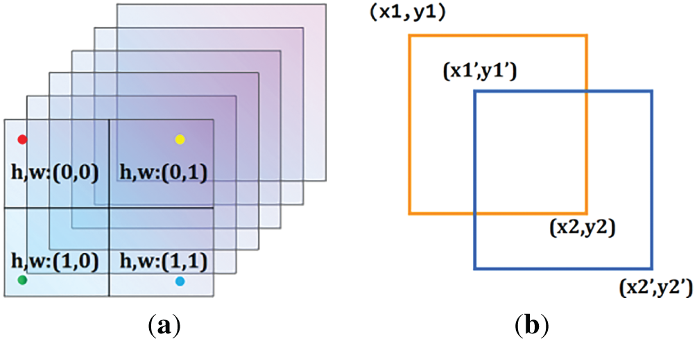
Figure 4: Graphical representation of image coordinate back-calculation

Based on the position of the proposed box and the offset value of the network output, the true value can be found, which is the yellow box in Fig. 4b, whose coordinates are calculated as follows:

x1=x1′+w′×offset_x1x2=x2′+w′×offset_x2y1=y1′+h′×offset_y1y2=y2′+h′×offset_y2(5)

In the formula above, index is the index value in the graph, strides is the step size of the slide and scale is the scaling ratio in the image pyramid, w, h are the width and height of the suggestion box and offset is the offset value predicted by the network.

MTCNN performs face detection and keypoint localization through an image pyramid and a cascade of three CNNs: P-Net, R-Net, and O-Net. P-Net performs feature extraction and classification through a sliding window to quickly identify face candidates and their locations. R-Net leverages deeper features to classify and regress the candidate regions, resulting in more accurate face bounding boxes. O-Net further refines the bounding boxes and precisely localizes facial keypoints. As shown in Fig. 5, the MTCNN effectively achieves the tasks of face detection and face keypoint localization using three cascaded networks that gradually screen and refine results.

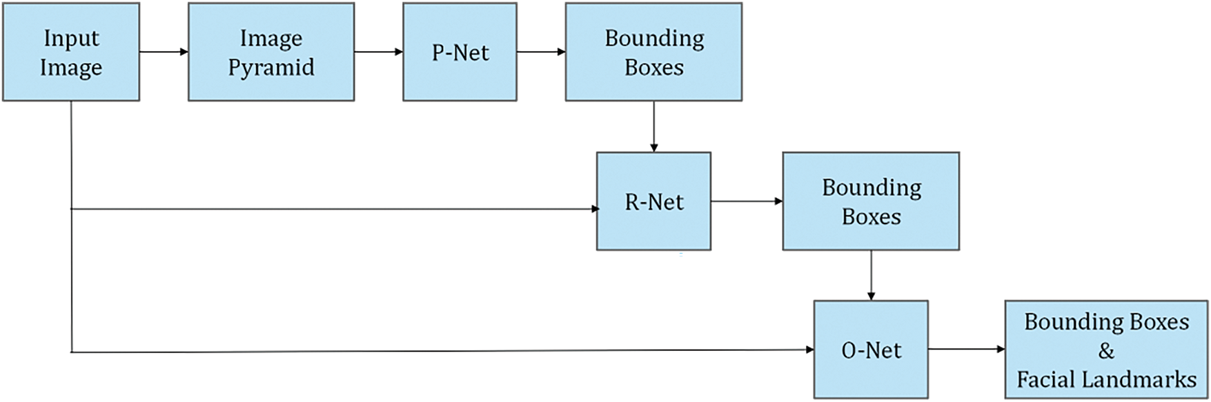
Figure 5: Complete flow of MTCNN

2.2.2 EfficientNet

EfficientNet achieves a balance of performance and efficiency through composite scaling that adjusts the width, depth, and resolution of the network. The model is pre-trained on large-scale image datasets to learn rich image features. These features can be applied to face feature extraction, accelerating model training and improving performance on face datasets. Fig. 6a shows the baseline EfficientNet structure, while Fig. 6b–d expand it in width, depth, and resolution. Fig. 6e illustrates the main idea: scaling all three dimensions together.

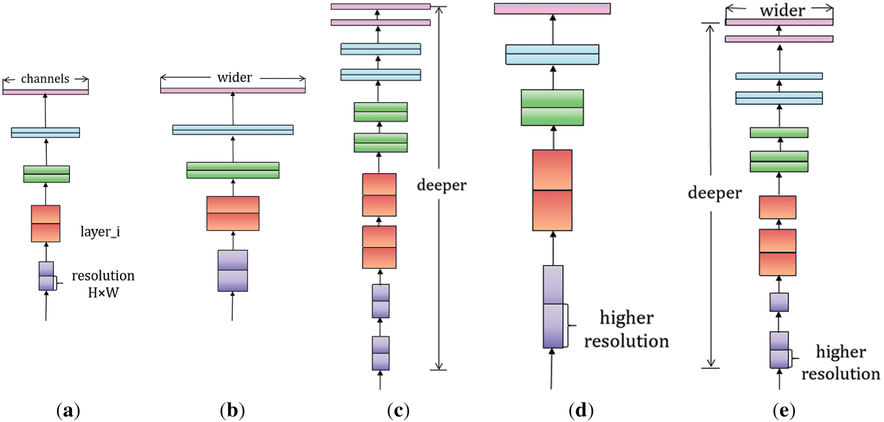
Figure 6: EfficientNet network structure. (a) baseline; (b) width scaling; (c) depth scaling; (d) resolution scaling; (e) compound scaling

Our target is to maximize the model accuracy for any given resource constraints, which can be formulated as an optimization problem:

maxd,w,rAccuracy(N(d,w,r))s.t.N(d,w,r)=⊙i=1⋯sF^id⋅L^i(X<r⋅Hi^,r⋅Wi^,w⋅C^i>X<r⋅H^i,r⋅W^i,w⋅C^i>)Memory(N)≤target_memoryFLOPs(N)≤target_flops(6)

Among these variables, d,w and r denote depth, width, and resolution multiplicity of the network. The subscripts 1…s indicate the serial number of the stage, and Fi denotes the convolution operation on the first layer of the convolution operation. Li means that Fi has Li convolutional layers with the same structure in the i-th stage. Memory represents the memory usage of the model. FLOPs are used as a constraint to balance model complexity and performance. By controlling the number of FLOPs, more efficient models can be designed with limited computational resources.

EfficientNet proposes a compound scaling method in which a mixing factor ϕ is used to unify the scaling depth, width and resolution parameter, which is calculated as follows:

Scale=ϕ×depthd×widthw×resolutionr(7)

2.3 Loss Function

2.3.1 Loss Function Used for Classification Task—Focal Loss

Focal Loss [24] is designed to address class imbalance, a common challenge in machine learning where some categories have significantly fewer samples. Unlike Cross-Entropy Loss [40], which treats all classes equally, Focal Loss reweights the loss to reduce the impact of well-classified or majority-class samples, thereby focusing more on difficult and minority-class examples.

The focal loss for binary classification is derived from the Cross-Entropy (CE) loss.

CE(p,y)={−log⁡(p)ify=1−log⁡(1−p)otherwise(8)

The y∈{±1} specifies the ground truth class, the p∈[0,1] is the estimated probability of the model for the class labeled y=1. Define pt:

pt={pify=11−potherwise(9)

Rewritten CE:

CE(p,y)=CE(pt)=−log⁡(pt)(10)

A remarkable property of this loss is that even easily categorized samples can produce losses of non-trivial magnitude. A common way to address class imbalances is to introduce a weighting factor α∈[0,1], the CE loss of the α equilibrium is written as:

CE(pt)=−αtlog⁡(pt)(11)

This loss is a extension of the CE, which we consider to be the experimental baseline for focal loss. Adding a modulation factor (1−pt)γ to the cross entropy loss with a tunable focusing paramete γ≥0, the α balanced focal loss is used. In summary, define the focal loss as:

FL(pt)=−αt(1−pt)γlog⁡(pt)(12)

The focal loss method operates by scaling the loss using an exponential function that incorporates the actual observed category probability to adjust the loss weight. For instances that are easily classified, the focus factor approaches 0, which in turn limits their impact on the overall loss. For samples that are difficult to categorize, they are given a larger focus factor, which increases their loss weight and influence in training. The introduction of a focus factor allows Focal Loss to effectively decrease the impact of the majority category and concentrate on the minority category, thereby enhancing the accuracy of predictions for the latter. In our implementation, we set the hyperparameters of Focal Loss to α = 0.5 and γ = 2, following standard practice in prior works, which offer a stable performance in our preliminary ablation experiments.

2.3.2 Loss Function Used for Regression Task—MSE

Mean Squared Error (MSE) Loss is commonly used in regression tasks [41] to measure the difference between predicted and true values. MSE is calculated by adding up the squares of the differences between them for each sample and dividing by the number of samples. The mathematical expression is given below:

MSE=1n∑i=1n(xi−yi)2(13)

MSE yields a non-negative output, and values closer to 0 reflect more accurate predictions made by the model. Since the square of the error is used in the MSE calculation, relatively large errors are magnified, making the model more sensitive to large errors. It is a continuously derivable loss function, which makes it possible to apply optimization algorithms such as gradient descent for parameter updating during the training process. Computation entails only the summation of squared differences and addition, resulting in low computational complexity.

3  Our Approach

3.1 Context Feature Extraction

When extracting emotional features from a scene, the entire image is fed into the channel. To capture crucial regions of the image, the CBAM attention mechanism is employed, which integrates channel and spatial attention mechanisms.

In this study, we choose ResNet18 [42] as the backbone network for both the body and context feature extraction channels. Compared with deeper models such as ResNet50 and ResNet101, ResNet18 achieves better performance while significantly reducing training time and computational resource usage. Its relatively simple architecture also makes it well-suited for integration with the CBAM attention mechanism.

Incorporating the CBAM attention mechanism on the network structure of ResNet18 can enhance the feature representation capability of the model. By adaptively learning the importance of channels and space, CBAM can provide a more accurate and robust feature representation, enabling the model to better capture the features that are most useful for the task. Fig. 7 shows the exact location of the CBAM module when it is integrated in a ResBlock. We apply CBAM to the convolutional output in each block.

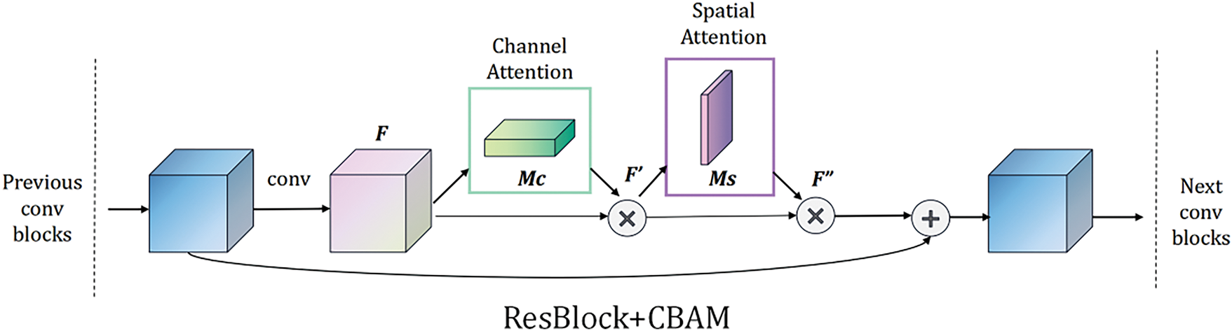
Figure 7: Exact location of ResBlock addition to the CBAM attention module

The complete network structure of context feature extraction channel after adding CBAM is shown in Fig. 8, the input of the channel is the original image that contains both characters and scenes. The CBAM attention module is added in all four stages of ResNet18, and finally the features of the scene channel are obtained through the average pooling layer and the fully connected layer.

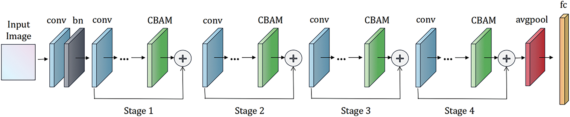
Figure 8: Schematic diagram of the ResNet18 network incorporating the CBAM attention module

3.2 Face Feature Extraction

Since more than 25% of the images in the EMOTIC dataset fail to detect clear faces, an adaptive face channel is introduced to perform face detection and feature extraction directly from body frames. As shown in Fig. 9, MTCNN is used to detect faces within the body bounding boxes. If one or more faces are detected, the extracted facial frames are input into EfficientNet for feature extraction. The features from the scene, body, and face channels are then fused for subsequent classification. If no face is detected, the face channel is deactivated (weight set to 0), and classification proceeds using only the body and context features.

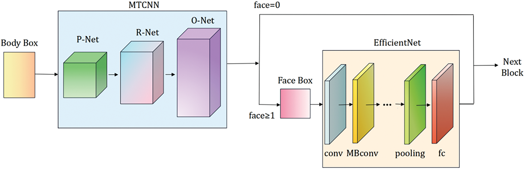
Figure 9: The structure of face feature extraction channel

3.3 Model Structural Design

The complete model structure of adaptive multi-channel image sentiment analysis network with Focal Loss (AMSA) is shown in Fig. 10.

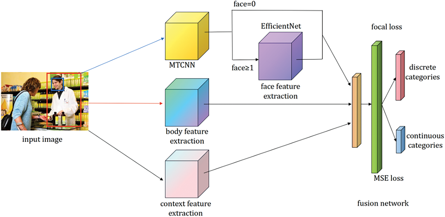
Figure 10: Complete model structure of AMSA

Both the body feature extraction module and the context feature extraction module use pre-trained ResNet18 models. Additionally, the context feature extraction part incorporates the CBAM attention mechanism to extract scene-relevant features. The face feature extraction part takes the body box as input. When a face is successfully detected by MTCNN, the corresponding facial region is extracted and processed by EfficientNet, and the features from all three channels (face, body, and context) are fused for classification. If no face is detected, the face channel is deactivated (the weight is set to zero), and the model switches to a dual-branch fusion mode, using only body and context features for emotion prediction. To ensure stable performance under both conditions, we adopt fixed fusion weights determined through validation set optimization. The fusion output y is computed as follows:

y=σ(0.4⋅fbody+0.6⋅fcontext)y=σ(0.5⋅fface+0.2⋅fbody+0.3⋅fcontext)(14)

Finally, the fusion network module combines the features from the three feature extraction modules and carries out fine-grained sentiment representation regression using two fully connected layers. The output results in both discrete and continuous dimensions.

4  Experiments

4.1 EMOTIC Dataset

The EMOTIC dataset is a collection of images of people in unconstrained environments, where over 25% of people’s faces are partially occluded or have very low resolution. It contains 23,571 images and 34,320 annotated characters. The dataset uses a combination of queries containing keywords for different locations, social environments, diverse activities, and various emotional states, and it provides manually annotated body regions. The annotations comprise 3 continuous emotion dimensions: Valence, Arousal, and Dominance and 26 discrete emotions: anticipation, engagement, confidence, happiness, surprise, fatigue, embarrassment, anger and more. The detailed definitions of these categories can be found in [13,43], and Fig. 11 shows example images of these categories.

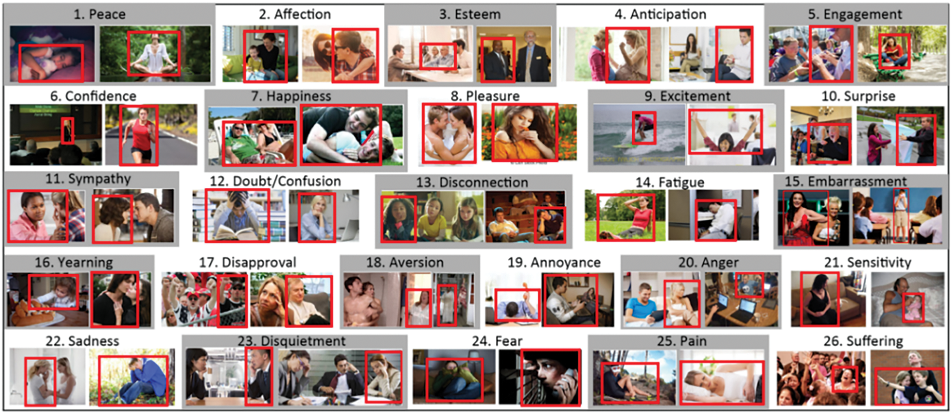
Figure 11: Example of discrete category annotated image from EMOTIC dataset [13]

In our experiment, the dataset is split into three subsets: 70% for training, 20% for validation, and 10% for testing. The split ensures a balanced distribution of emotion categories across the subsets.

Images are annotated according to the VAD model [44], which represents emotions through a combination of three continuous dimensions, each of which is an integer value within the range of 1 to 10. The VAD model is defined as follows: valence (V) is used to measure the degree of positivity or pleasantness of an emotion, ranging from negative to positive; arousal (A) is used to measure an individual’s degree of arousal, ranging from inactive/calm to agitated/ready for action; and dominance (D) is used to measure a person’s degree of control over a situation, ranging from non-control to control. Fig. 12 illustrates the various values assigned to each dimension.

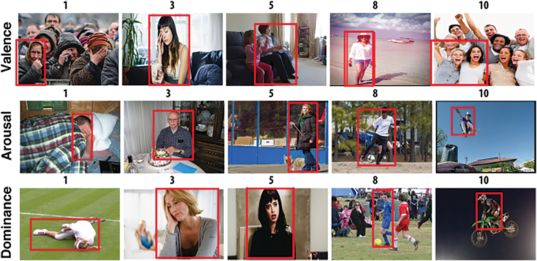
Figure 12: Example of continuous dimension annotated image from EMOTIC dataset [13]

We utilize average precision (AP) to measure the performance of discrete category classification and the Jaccard coefficient (JC) [45] to test the similarity between two sets. Due to the classification of EMOTIC dataset belongs to multi-label classification, the final output may have some overlap with Ground Truth or vary completely. Therefore, we use JC to represents the ratio of the size of the intersection of A and B to the size of the concatenation of A and B. It is defined by Eq. (15), the higher the JC, the better the result. The maximum value of the JC is 1, where the detected category and the Ground Truth category are identical.

JC(A,B)=|A∩B||A∪B|=|A∩B||A|+|B|−|A∩B|(15)

Performance of VAD in three continuous dimensions is measured through the MAE. A lower calculated value indicates a smaller error and better predictive performance of the model as defined in Eq. (16).

MAE=1m∑i=1m|yi−f(xi)|(16)

The distribution of the 26 emotion categories in the EMOTIC dataset is presented in Fig. 13, with a descending order from left to right.

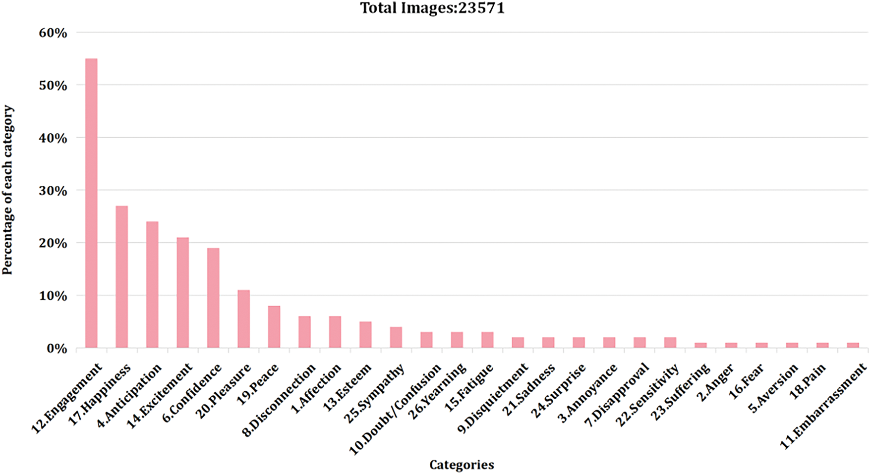
Figure 13: Percentage of each category in the dataset

4.2 Analysis of Results

To evaluate the contribution of each module in our model, we conducted an ablation study involving various combinations of CBAM, the adaptive face channel, and Focal Loss in six experimental configurations. As shown in Table 1, the results demonstrate that each module contributes positively to the overall performance. (iii) and (iv) demonstrate the benefit of incorporating adaptive face recognition channel and confirm that the focal loss effectively enhanced performance on imbalanced data. And the full AMSA model achieves the highest accuracy, while configurations with only partial components show reduced performance.

To evaluate our model on a fine-grained dimension, we conducted classification experiments on 26 discrete emotion categories and compared our AMSA model with several representative methods, including those proposed by Zhang et al. [14], Lee et al. [15], Mittal et al. [16], Kosti et al. [43], Wang et al. [46], Li et al. [47] and Yang et al. [48].

As shown in Table 2, AMSA achieved the highest mean Average Precision (mAP), which was 2.53% higher than that of the best baseline paper [48]. This significant improvement demonstrates the effectiveness of the proposed adaptive multi-channel framework. Additionally, our model achieved the highest classification accuracy in 10 emotion categories, including Anger, Annoyance, and others. These gains can be attributed to the introduction of Focal Loss, which addresses the class imbalance issue in the EMOTIC dataset by giving more weight to underrepresented classes during training. This is especially important given the unbalanced distribution of emotion categories in the dataset. Moreover, we observed that in complex scene categories with subtle emotional cues, such as Annoyance and Sympathy, our model achieved 24.22% and 35.30%, respectively, significantly outperforming other methods. This confirms that our model does not overly rely on a single modality, but is capable of adapting to diverse visual cues present in complex scenes.

In addition to the aforementioned models, several studies have reported only the mAP without disclosing the classification accuracy for individual emotion categories. For completeness, we provide a comparative summary of these results in Table 3. de Lima Costa et al. [49] proposed a lightweight single-stream model focused on computational efficiency, but showed limited accuracy improvement. Etesam et al. [50] adopted a large language model for caption-based reasoning. Zhang et al. [51] proposed a training paradigm that extracts visual affective cues from communication using unedited data and topic-aware contextual encoding. In contrast, our AMSA reaches the highest mAP of 35.04%, wihch shows a balanced and accurate recognition result across both common and rare classes.

To evaluate our model in the continuous emotional dimension, we conducted regression analysis on the VAD space. As shown in Table 4, our model achieves a 10% lower average error rate compared to [43], and performs comparably to [14]. This result proves the effectiveness of using Mean Squared Error (MSE) loss in our regression setting. Compared to both approaches, AMSA adopts a more comprehensive image analysis framework by incorporating adaptive face detection and multi-channel feature fusion. Unlike [43], which uses SL1 Loss, our method leverages MSE Loss to better optimize continuous predictions. While Zhang et al. [14] also adopt MSE, AMSA achieves similar overall performance in average error but exhibits more balanced results across the three VAD dimensions.

To provide a more intuitive result for our experiment, we displays three representative samples from the EMOTIC dataset in Table 5, including two successful cases and one challenging case with facial occlusion. The classification predictions are denoted in black for agreeing with those in Ground Truth, and in red for misclassification. We evaluated the results’ efficacy using JC coefficients and MAE. Our model correctly detects the majority of ground-truth categories in the first two examples. Compared to [43], the JC coefficients are improved by 0.15 and 0.30, respectively, while the MAE values are reduced by 1.23 and 1.57. In the third case, the face was obscured and model relied solely on body and context features for judgment, so it is not very accurate in terms of emotions, resulting in misjudgments such as fear and pain. Although its performance has declined, the gap compared to [43] remains small. This indicates the validity of the AMSA model presented in this paper.

This example also shows the importance of our adaptive strategy. When the face is blocked, the model automatically switches to rely more on body and context features. Although this fallback approach cannot fully replace facial information, it still enables the model make reasonable predictions by using other visual cues in the image.

5  Conclusion

In this paper, we proposed AMSA, a multi-channel model for contextual sentiment analysis that adaptively integrates facial, body, and scene features. The face channel leverages MTCNN and EfficientNet, while the body and context channels employ ResNet18, with CBAM attention further enhancing scene-level feature extraction. To address class imbalance in the EMOTIC dataset, we adopt Focal Loss for classification and MSE Loss for regression. Experimental results demonstrate that AMSA outperforms previous methods by 2.63% in average accuracy, and our model achieves leading performance on several underrepresented emotion categories, confirming the effectiveness of the proposed architecture and loss function.

In the future, this work can be extended to applications such as intelligent surveillance, human-computer interaction, supporting the practical deployment of image-based sentiment analysis. Further research will focus on improving the model’s generalization in cross-domain scenarios and exploring the integration of textual and audio modalities for more comprehensive multimodal sentiment analysis.

Acknowledgement: Not applicable.

Funding Statement: The authors received no specific funding for this study.

Author Contributions: The authors confirm contribution to the paper as follows: Conceptualization, Xiaofang Jin; methodology, Yiran Li; software, Yiran Li; validation, Yuying Yang; data curation, Yuying Yang; writing—original draft preparation, Yuying Yang, Yiran Li; writing—review and editing, Xiaofang Jin, Yiran Li, Yuying Yang. All authors reviewed the results and approved the final version of the manuscript.

Availability of Data and Materials: The authors confirm that the data supporting the findings of this study are available within the article [13].

Ethics Approval: Not applicable.

Conflicts of Interest: The authors declare no conflicts of interest to report regarding the present study.

References

1. Picard RW. Affective computing. Cambridge, MA, USA: MIT Press; 1995. [Google Scholar]

2. Wang L, Niu J, Yu S. SentiDiff: combining textual information and sentiment diffusion patterns for twitter sentiment analysis. IEEE Trans Knowl Data Eng. 2020;32(10):2026–39. doi:10.1109/tkde.2019.2913641. [Google Scholar] [CrossRef]

3. Er MB. A novel approach for classification of speech emotions based on deep and acoustic features. IEEE Access. 2020;8:221640–53. doi:10.1109/ACCESS.2020.3043201. [Google Scholar] [CrossRef]

4. Liu X, Wang M. Context-aware attention network for human emotion recognition in video. Adv Multimedia. 2020;2020:8843413. doi:10.1155/2020/8843413. [Google Scholar] [CrossRef]

5. Jayaraman S, Mahendran A. An improved facial expression recognition using CNN-BiLSTM with attention mechanism. Int J Adv Comput Sci. 2024;15(5):1–10. doi:10.14569/IJACSA.2024.01505132. [Google Scholar] [CrossRef]

6. Slogrove K, van der Haar D. Group emotion recognition in the wild using pose estimation and LSTM neural networks. In: Proceedings of the International Conference on Artificial Intelligence, Big Data, Computing and Data Communication Systems (ICABCD); 2022 Aug 4–5; Durban, South Africa. p. 1–6. [Google Scholar]

7. Liu S, Zhang X, Li Y, Chen H, Wang Q, Zhao Y, et al. 3DCANN: a spatio-temporal convolution attention neural network for EEG emotion recognition. IEEE J Biomed Health Inform. 2022;26(11):5321–31. doi:10.1109/jbhi.2021.3083525. [Google Scholar] [PubMed] [CrossRef]

8. Liu Z, Braytee A, Anaissi A, Zhang G, Qin L, Akram J. Ensemble pretrained models for multimodal sentiment analysis using textual and video data fusion. In: Proceedings of the WWW'24: Companion Proceedings of the ACM Web Conference 2024; 2024 May 13–17; Singapore. p. 1841–48. [Google Scholar]

9. Wu S, Wang X, Wang L, He D, Dang J. Enriching multimodal sentiment analysis through textual emotional descriptions of visual-audio content. In: Proceedings of the Thirty-Ninth AAAI Conference on Artificial Intelligence (AAAI); 2025 Feb 25–Mar 4; Philadelphia, PA, USA. p. 1601–9. [Google Scholar]

10. Shi P, Hu M, Nakagawa S, Liu Y, Wang F, Zhang Z, et al. Text-guided reconstruction network for sentiment analysis with uncertain missing modalities. IEEE Trans Affect Comput. 2025:1–15. doi:10.1109/taffc.2025.3541743. [Google Scholar] [CrossRef]

11. Xie Z, Yang Y, Wang J, Liu X, Li X. Trustworthy multimodal fusion for sentiment analysis in ordinal sentiment space. IEEE Trans Circuits Syst Video Technol. 2024;34(8):7657–70. doi:10.1109/tcsvt.2024.3376564. [Google Scholar] [CrossRef]

12. Li Y, Zhu R, Li W. CorMulT: a semi-supervised modality correlation-aware multimodal transformer for sentiment analysis. arXiv:2407.07046. 2024. [Google Scholar]

13. Kosti R, Alvarez JM, Recasens A, Lapedriza A. Emotion recognition in context. In: 2017 IEEE Conference on Computer Vision and Pattern Recognition (CVPR); 2017 Jul 21–26; Honolulu, HI, USA. p. 1960–8. [Google Scholar]

14. Zhang M, Liang Y, Ma H. Context-aware affective graph reasoning for emotion recognition. In: Proceedings of the IEEE International Conference on Multimedia and Expo (ICME 2019); 2019 Jul 8–12; Shanghai, China. p. 151–6. [Google Scholar]

15. Lee J, Kim S, Kim S, Park J, Sohn K. Context-aware emotion recognition networks. In: Proceedings of the IEEE/CVF International Conference on Computer Vision (ICCV); 2019 Oct 27–Nov 2; Seoul, Republic of Korea. p. 10142–51. [Google Scholar]

16. Mittal T, Guhan P, Bhattacharya U, Chandra R, Bera A, Manocha D. EmotiCon: context-aware multimodal emotion recognition using Frege’s principle. In: Proceedings of the IEEE Conference on Computer Vision and Pattern Recognition (CVPR); 2020 Jun 13–19; Seattle, WA, USA. p. 14234–43. [Google Scholar]

17. Wu S, Zhou L, Hu Z, Liu J. Hierarchical context-based emotion recognition with scene graphs. IEEE Trans Neural Netw Learn Syst. 2024;35(3):3725–39. doi:10.1109/tnnls.2022.3196831. [Google Scholar] [PubMed] [CrossRef]

18. He H, Garcia EA. Learning from imbalanced data. IEEE Trans Knowl Data Eng. 2009;21(9):1263–84. doi:10.1109/tkde.2008.239. [Google Scholar] [CrossRef]

19. Cheng K, Zhang C, Yu H, Yang X, Zou H, Gao S. Grouped SMOTE with noise filtering mechanism for classifying imbalanced data. IEEE Access. 2019;7:170668–81. doi:10.1109/access.2019.2955086. [Google Scholar] [CrossRef]

20. Zhang X, Zhu C, Wu H, Liu Z, Xu Y. An imbalance compensation framework for background subtraction. IEEE Trans Multimedia. 2017;19(11):2425–38. doi:10.1109/tmm.2017.2701645. [Google Scholar] [CrossRef]

21. Bader-El-Den M, Teitei E, Perry T. Biased random forest for dealing with the class imbalance problem. IEEE Trans Neural Netw Learn Syst. 2019;30(7):2163–72. doi:10.1109/tnnls.2018.2878400. [Google Scholar] [PubMed] [CrossRef]

22. Zhang K, Zhang Z, Li Z, Qiao Y. Joint face detection and alignment using multitask cascaded convolutional networks. IEEE Signal Process Lett. 2016;23(10):1499–503. doi:10.1109/lsp.2016.2603342. [Google Scholar] [CrossRef]

23. Tan M, Le QV. EfficientNet: rethinking model scaling for convolutional neural networks. arXiv:1905.11946. 2020. [Google Scholar]

24. Lin TY, Goyal P, Girshick R, He K, Dollár P. Focal loss for dense object detection. IEEE Trans Pattern Anal Mach Intell. 2020;42(2):318–27. doi:10.1109/tpami.2018.2858826. [Google Scholar] [PubMed] [CrossRef]

25. Yang J, Gao X, Li L, Wang X, Ding J. SOLVER: scene-object interrelated visual emotion reasoning network. IEEE Trans Image Process. 2021;30:8686–701. doi:10.1109/tip.2021.3118983. [Google Scholar] [PubMed] [CrossRef]

26. Pikoulis I, Filntisis PP, Maragos P. Leveraging semantic scene characteristics and multi-stream convolutional architectures in a contextual approach for video-based visual emotion recognition in the wild. In: Proceedings of the 16th IEEE International Conference on Automatic Face and Gesture Recognition (FG); 2021 May 15–18; Jodhpur, India. p. 1–8. [Google Scholar]

27. Yuan Y, Lu F, Cheng X, Liu Y. Context based vision emotion recognition in the wild. In: Proceedings of the 17th IEEE Conference on Industrial Electronics and Applications (ICIEA); 2022 Dec 16–19; Chengdu, China. p. 479–84. [Google Scholar]

28. Hu J, Shen L, Albanie S, Sun G, Wu E. Squeeze-and-excitation networks. IEEE Trans Pattern Anal Mach Intell. 2020;42(8):2011–23. doi:10.1109/tpami.2019.2913372. [Google Scholar] [PubMed] [CrossRef]

29. Woo S, Park J, Lee JY. CBAM: convolutional block attention module. In: Ferrari V, Hebert M, Sminchisescu C, Weiss Y, editors. Computer vision—ECCV 2018. Cham, Switzerland: Springer; 2018. p. 3–19. doi:10.1007/978-3-030-01234-2_1. [Google Scholar] [CrossRef]

30. Freund Y, Schapire RE. A decision-theoretic generalization of on-line learning and an application to boosting. J Comput Syst Sci. 1997;55(1):119–39. doi:10.1006/jcss.1997.1504. [Google Scholar] [CrossRef]

31. Cortes C, Vapnik V. Support-vector networks. Mach Learn. 1995;20(3):273–97. doi:10.1023/a:1022627411411. [Google Scholar] [CrossRef]

32. Viola PA, Jones MJ. Rapid object detection using a boosted cascade of simple features. In: Proceedings of the 2001 IEEE Computer Society Conference on Computer Vision and Pattern Recognition, CVPR 2001; 2001 Dec 8–14; Kauai, HI, USA. [Google Scholar]

33. Jabade V, Ingale A, Joshi R. Robust face detection and identification using HOG-based features and machine learning. In: Proceedings of the 2023 2nd International Conference on Futuristic Technologies (INCOFT); 2023 Nov 2–3; Coimbatore, India. p. 1–6. [Google Scholar]

34. Ren S, He K, Girshick R, Sun J. Faster R-CNN: towards real-time object detection with region proposal networks. IEEE Trans Pattern Anal Mach Intell. 2017;39(6):1137–49. doi:10.1109/tpami.2016.2577031. [Google Scholar] [PubMed] [CrossRef]

35. Turk M, Pentland A. Eigenfaces for recognition. J Cogn Neurosci. 1991;3(1):71–86. [Google Scholar] [PubMed]

36. Tan X, Triggs B. Enhanced local texture feature sets for face recognition under difficult lighting conditions. IEEE Trans Image Process. 2010;19(6):1635–50. doi:10.1109/tip.2010.2042645. [Google Scholar] [PubMed] [CrossRef]

37. Umer S, Rout RK, Tiwari S, AlZubi AA, Alanazi JM, Yurii K. Human-computer interaction using deep fusion model-based facial expression recognition system. Comput Model Eng Sci. 2023;135(2):1165–85. doi:10.32604/cmes.2022.023312. [Google Scholar] [CrossRef]

38. Parkhi OM, Vedaldi A, Zisserman A. Deep face recognition. In: Proceedings of the British Machine Vision Conference (BMVC); 2015 Sep 7–10; Swansea, UK. [Google Scholar]

39. Felzenszwalb P, Girshick R, McAllester D, Ramanan D. Object detection with discriminatively trained part-based models. IEEE Trans Pattern Anal Mach Intell. 2010;32(9):1627–45. doi:10.1109/tpami.2009.167. [Google Scholar] [PubMed] [CrossRef]

40. Sangari A, Sethares W. Convergence analysis of two loss functions in soft-max regression. IEEE Trans Signal Process. 2016;64(5):1280–8. doi:10.1109/tsp.2015.2504348. [Google Scholar] [CrossRef]

41. Zhao H, Shi J, Qi X, Wang X, Jia J. Pyramid scene parsing network. In: Proceedings of the IEEE Conference on Computer Vision and Pattern Recognition (CVPR); 2017 Jun 21–26; Honolulu, HI, USA. p. 6230–9. [Google Scholar]

42. He K, Zhang X, Ren S, Sun J. Deep residual learning for image recognition. In: Proceedings of the IEEE Conference on Computer Vision and Pattern Recognition (CVPR); 2016 Jun 27–30; Las Vegas, NV, USA. p. 770–8. [Google Scholar]

43. Kosti R, Alvarez JM, Recasens A, Lapedriza A. Context based emotion recognition using EMOTIC dataset. IEEE Trans Pattern Anal Mach Intell. 2020;42(11):2755–66. doi:10.1109/tpami.2019.2916866. [Google Scholar] [PubMed] [CrossRef]

44. Russell JA. A circumplex model of affect. J Pers Soc Psychol. 1980;39(6):1161–78. [Google Scholar]

45. Jaccard P. The distribution of the flora in the alpine zone. New Phytol. 1902;2:37–50. [Google Scholar]

46. Wang Z, Lao L, Zhang X, Li Y, Zhang T, Cui Z. Context-dependent emotion recognition. J Vis Commun Image Represent. 2022;89:103679. [Google Scholar]

47. Li W, Dong X, Wang Y. Human emotion recognition with relational region-level analysis. IEEE Trans Affect Comput. 2023;14(1):650–63. doi:10.1109/taffc.2021.3064918. [Google Scholar] [CrossRef]

48. Yang D, Yang K, Li M, Wang S, Wang S, Zhang L. Robust emotion recognition in context debiasing. In: Proceedings of the IEEE/CVF Conference on Computer Vision and Pattern Recognition (CVPR); 2024 Jun 16–22; Seattle, WA, USA. p. 12447–57. [Google Scholar]

49. de Lima Costa W, Talavera E, Figueiredo LS, Teichrieb V. High-level context representation for emotion recognition in images. In: Proceedings of the IEEE/CVF Conference on Computer Vision and Pattern Recognition (CVPR); 2023 Jun 17–24. Vancouver, BC, Canada. p. 326–34. [Google Scholar]

50. Etesam Y, Yalçın ÖN, Zhang C, Lim A. Contextual emotion recognition using large vision language models. In: Proceedings of the 2024 IEEE/RSJ International Conference on Intelligent Robots and Systems (IROS); 2024 Oct 14–18; Abu Dhabi, United Arab Emirates. p. 4769–76. [Google Scholar]

51. Zhang S, Pan Y, Wang JZ. Learning emotion representations from verbal and nonverbal communication. In: Proceedings of the IEEE/CVF Conference on Computer Vision and Pattern Recognition (CVPR); 2023 Jun 17–24; Vancouver, BC, Canada. p. 18993–9004. [Google Scholar]