Fault Diagnosis of Wind Turbine Blades Based on Multi-Sensor Weighted Alignment Fusion in Noisy Environments

1  Introduction

Wind turbines are clean energy devices that convert wind energy into electricity, primarily composed of key components such as the tower, nacelle, generator, and blades. Among these, the blades serve as the core component and main power source of the turbine, and their maintenance level directly determines the power generation performance of the entire unit [1]. Modern wind turbine blades are typically designed with aerodynamic principles to maximize wind energy capture and drive the generator operation [2]. Consequently, the performance of the blades directly influences the energy conversion efficiency, power output, and overall economic benefits of the turbine [3,4].

Due to the long-term operation of wind turbines in complex outdoor environments, the blades face multiple severe challenges. During continuous operation, the blades are not only subjected to complex and variable wind loads but also endure environmental factors such as daily temperature variations, low temperatures, and rainwater erosion, which can lead to failures and affect the operational safety of the generating unit [5–7]. Therefore, real-time monitoring and fault diagnosis of blade operational status are of critical importance to ensure the safe and stable operation of wind turbine systems [8–10].

Deep learning models possess powerful learning capabilities and can capture complex fault features in an end-to-end manner, gradually becoming a mainstream approach for wind turbine blade fault diagnosis [11,12]. For example, Wei et al. [13] proposed a bidirectional long short-term memory model incorporating a Dropout mechanism (MBiLSTM-D) to enhance generalizability across different wind turbines, achieving accurate blade fault diagnosis. Sethi et al. [14] introduced a method combining continuous wavelet transform (CWT) with convolutional neural networks (CNN) for diagnosing wind turbine blade faults. Pan et al. [15] proposed a spatiotemporal joint processing framework integrating graph Fourier transform and deep learning to detect blade faults. Guo et al. [16] developed a semi-supervised fault diagnosis framework based on graph contrastive learning (GCL), which demonstrated superior diagnostic performance and generalization compared to traditional methods.

Despite these advances, deep learning still faces significant challenges in blade fault diagnosis. Firstly, noise in signals collected during blade operation obscures fault features, severely impacting the diagnostic performance of deep learning models [17]. Signals acquired in practical blade operation contain substantial and complex noise, including mechanical noise from components such as gears and bearings, interaction noise between blades and air, and noise caused by variations in sensor sensitivity. These noises significantly interfere with feature representation, dilute original fault characteristics, and make it difficult to detect weak or incipient faults. Strong noise may also mislead the model into recognizing noise as fault features, resulting in numerous misdiagnoses and considerably compromising diagnostic effectiveness [18–20].

Secondly, excessive reliance on single-sensor data in current blade fault diagnosis methods limits the acquisition of multidimensional state information, failing to comprehensively reflect the true health condition of such a complex system [21–23]. Modern large-scale wind turbine blades exhibit complex vibration patterns, and sensors in different directions, positions, or configurations capture fault features with considerable variation. For instance, if a blade fault induces periodic impacts in the x-direction, an accelerometer in the y-direction would have limited capability to capture such fault information. More critically, if the sensor itself experiences drift or failure, the entire diagnostic system would become ineffective. This single-point dependency significantly reduces monitoring reliability [24–26].

To address these issues, a multi-sensor fusion-based fault diagnosis method is proposed. Firstly, a Weight-Aligned Data Fusion Module is designed to comprehensively and effectively utilize multi-sensor fault information. This module begins by concatenating data from multiple sensors, then employs Squeeze-and-Excitation (SE) units [27] to linearly transform information from each channel into weights, achieving weight alignment. Finally, the self-attention mechanism and feedforward neural network of the Transformer encoder are utilized to achieve deep-level integration of multi-channel data. The module adaptively assigns appropriate weights to each channel, enabling magnitude alignment while achieving deep-level integration through key components of the Transformer. Compared to traditional methods such as weighted summation or simple concatenation, this approach offers higher utilization efficiency.

Secondly, a CNN-Transformer Coupled Feature Learning Architecture is constructed to enhance the ability to learn complex features under noisy conditions. A noisy environment blurs the waveform of original signals, obscures fault features, and even reduces the distinguishability between normal and fault signals. In the CNN-Transformer coupled architecture, CNNs excel at capturing fine-grained features and enable hierarchical feature learning, demonstrating strong representational capacity for complex and hidden characteristics, while Transformers possess global receptive fields and powerful feature modeling capabilities owing to their ability to perform feature interactions across arbitrary positions despite noise interference. By combining the strengths of both, the CNN-Transformer Coupled Feature Learning Architecture can analyze sample information from a global perspective in noisy environments while retaining the ability to focus on fine-grained features and mine complex patterns. Compared to other methods combining CNNs and Transformers, the novelty of the proposed method lies in utilizing CNN as an embedding approach to adjust dimensions, intertwined with the Transformer architecture, thereby achieving iterative feature enhancement and dimensionality elevation [28].

The structure of this paper is as follows: Section 2 briefly introduces relevant theories. Section 3 elaborates on the proposed method. Section 4 provides experimental validation through case studies, and Section 5 concludes the paper and outlines future research directions.

2  Basic Theory

2.1 Transformer Encoder

The Transformer Encoder [29] consists of N identical encoder layers stacked together, where the output of each encoder layer serves as the input to the next, ultimately producing a contextual representation of the entire input sequence [30].

Each encoder layer contains two core sub-layers: a multi-head self-attention mechanism and a feedforward neural network. Each of these sub-layers is surrounded by a residual connection, followed immediately by a layer normalization operation. This structure offers advantages in parallel processing and context-aware representation. The architecture of the Encoder is illustrated in Fig. 1 [31,32].

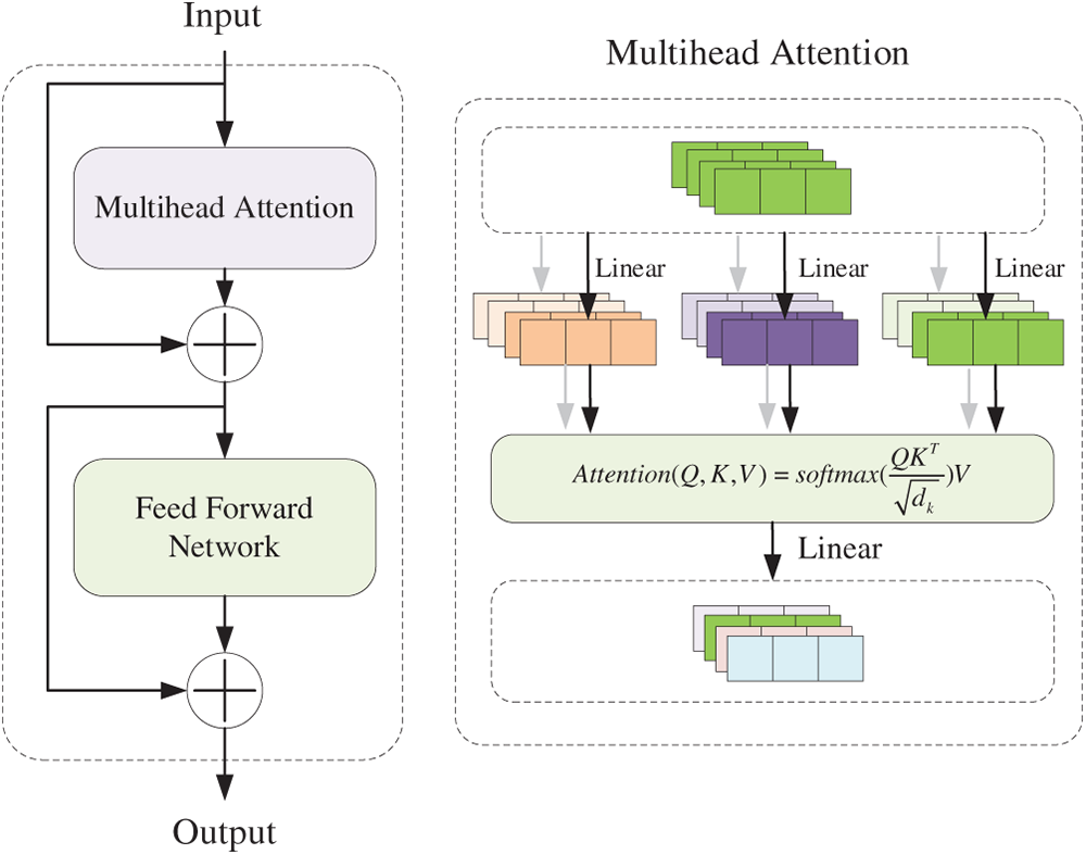
Figure 1: The architecture of transformer encoder

The core of the multi-head self-attention mechanism is the Scaled Dot-Product Attention. For a given input Zl−1, query (Q), key (K), and value (V) matrices are first generated through linear transformations.

Q=Zl−1WQ,K=Zl−1WK,V=Zl−1WV(1)

Next, the attention weights and output are computed:

Attention(Q,K,V)=softmax(QKTdk)V(2)

where dk is the dimension of K and V. The attention mechanism in Transformer operates through multi-head computation: the outputs of all attention heads are concatenated and then linearly transformed to produce the final multi-head self-attention output:

Hi=Attention(Qi,Ki,Vi)MHSA=Concat(H1,H2,Hh)Wo(3)

where Hi is the output of Attention, MHSA denotes the output of the multi-head self-attention mechanism. Following the attention output, a residual connection is incorporated, effectively mitigating the gradient vanishing problem and enabling the Transformer model to achieve greater potential depth [33].

Zattn(l)=LayerNorm(Z(l−1)+MHSA(Z(l−1)))(4)

Subsequently, the feedforward neural network (FFN) operation is performed to further facilitate feature learning. The FFN projects the features into a hidden layer and then restores them to the original dimension. Its computation is as follows:

FFN(Z)=(relu(ZW1+b1))W2+b2(5)

Finally, the output of the Transformer Encoder is obtained through the residual connection.

2.2 Squeeze-and-Excitation Module

The Squeeze-and-Excitation [34] (SE) module adaptively learns the importance of each channel and reweights the feature maps accordingly. Its structure is illustrated in Fig. 2.

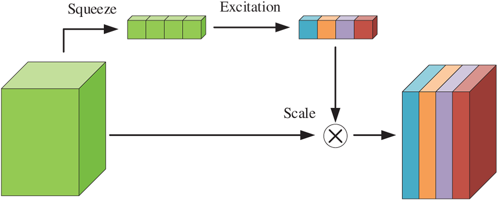
Figure 2: The squeeze-and-excitation (SE) module

The computation of the SE module involves three steps, elaborated below:

Squeeze Operation: The input feature with dimensions (H, W, C) undergoes global average pooling along the spatial dimensions, resulting in an output of size (1, 1, C):

zc=1H×W∑i=1H∑j=1Wuc(i,j)(6)

where zc is the c-th element of the Squeeze output z, uc represents the data of the c-th channel in the output feature map.

Excitation Operation: Utilizing the information extracted by the Squeeze operation and capturing interdependencies between channels, this step computes the weight of each channel through linear layers. Specifically, the input is first projected into a hidden layer with ReLU activation to introduce non-linearity, and then projected to the output layer where a sigmoid function is applied for normalization:

s=sigmoid(W2⋅relu(W1z))(7)

where s is the output of the Excitation operation.

Feature Weighting: Multiply the weight values calculated by Excitation by the corresponding channel data to obtain weighted features:

yc=scuc(8)

where yc is the output of channel c.

3  Proposed Method

3.1 CNN-Transformer Coupled Feature Learning Architecture Design

Traditional deep learning models, such as CNN and Transformer, still suffer limitations in the field of mechanical fault diagnosis. The pooling layer in CNN tends to lose key information, and due to the fixed size of the convolution kernel, the receptive field of CNN is limited, making it unable to achieve long-range dependencies. While Transformers can enable global information interaction, their computational complexity is higher, and they require a large amount of fault data.

Thus, a CNN-Transformer coupled feature learning architecture is proposed, as shown in Fig. 3.

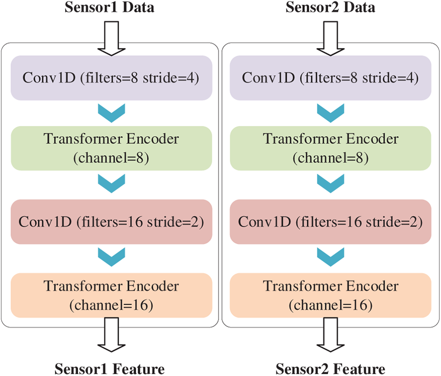
Figure 3: CNN-transformer coupled feature learning architecture

The CNN-Transformer coupled feature learning architecture can be used for multi-sensor data input. Taking Fig. 3 as an example, the raw data from Sensor 1 and Sensor 2 are processed through two parallel CNN-Transformer modules, respectively, yielding two features for subsequent data fusion. For wind turbine fault diagnosis tasks, the data typically consists of one-dimensional time-series vibration signals. Therefore, convolution operations are used to upscale the one-dimensional signals, resulting in 8-channel data (similar to the embedding in traditional Transformers). This data is then input into the first Transformer Encoder model for processing. Repeating this process yields a 16-dimensional output feature.

The hyperparameter settings for the CNN-Transformer Coupled Feature Learning Architecture are shown in Table 1. The first Conv1D achieves both feature extraction and downsampling. Setting the stride to 4 aims to quickly extract effective information with a larger stride, saving the subsequent computation of the model, and setting filter = 8 realizes preliminary dimension increase to prepare for matching the Transformer encoder. The Transformer encoder sets the number of attention heads to 2 because the dimension is small, which can reduce some redundant computation. At the same time, ffn_dim is set to twice the input dimension to fully extract more hidden features. Subsequently, the second CNN further increases the dimension to expand feature information, and then the Transformer encoder processes the output.

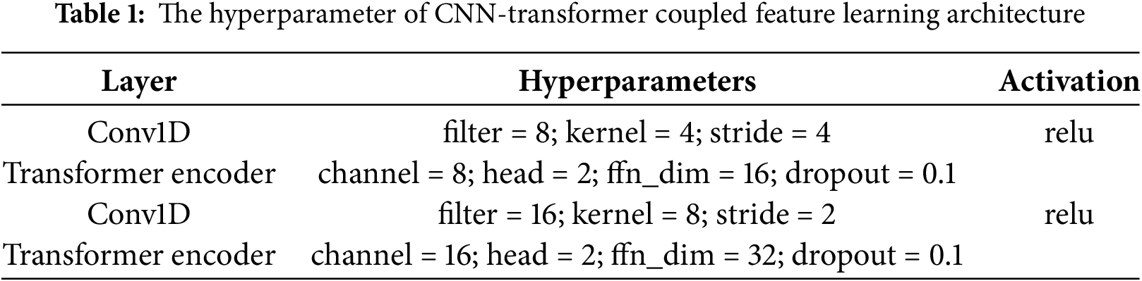
Remarks: filter refers to the number of convolutional kernels, kernel refers to the size of the convolutional kernel, channel refers to the input dimension, head refers to the number of heads, and ffn_dim refers to the dimension of the FFN hidden layer.

Assuming an input data size of (512, 1), after passing through the first convolutional layer, its dimensions change to (128, 8), achieving dimension expansion and downsampling. Then, the dimensions remain unchanged after passing through the Transformer Encoder layer, followed by the second convolutional layer, which converts the dimensions to (64, 16), and the output is generated by the Transformer Encoder. It can be observed that the features output by the CNN-Transformer coupled feature learning architecture possess certain spatial characteristics, which are advantageous for subsequent weight alignment and fusion.

3.2 Weight-Aligned Data Fusion Module Construction

This study constructs a Weight-Aligned Data Fusion Module to effectively fuse these features from different sources. Fig. 4 shows the structural diagram of the Weight-Aligned Data Fusion Module. As shown in the figure, the first step involves concatenating features from multiple sources:

Fc=concat(F1,F2)(9)

where Fc is the merged features, F1 and F2 are the features calculated by the CNN-Transformer coupled feature learning architecture before merging.

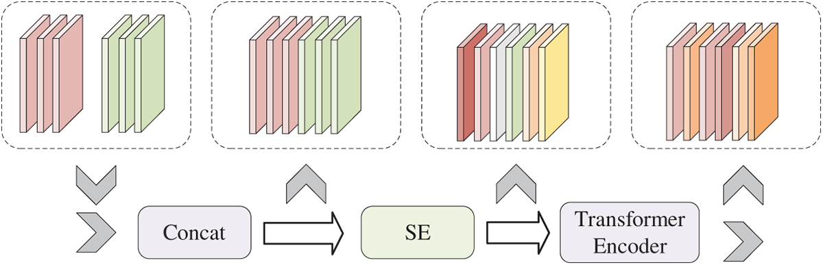
Figure 4: Weight-aligned data fusion module

After feature concatenation, a higher-dimensional tensor is formed. Since the two sets of tensors originate from different sensors, there are differences in data distribution between different channels. Therefore, the SE unit needs to learn and weigh the channels to align multi-source data and reduce the impact of excessive differences in parallel feature extraction:

F~c=SE(Fc)(10)

The SE module alone can only achieve weighting of each channel, but does not achieve true fusion between channels. Therefore, the output mixed features of SE require Transformer Encoder operations to obtain the final fusion output. The Transformer Encoder, via self-attention, efficiently captures long-range dependencies, dynamically emphasizes critical aligned features, and models global patterns—advantages that make it more suitable for deep feature learning after weight alignment, compared with structures like CNNs and fully connected layers.

Fo=TransformerEncoder(F~c)(11)

Table 2 lists the hyperparameters for the Weight-Aligned Data Fusion Module.

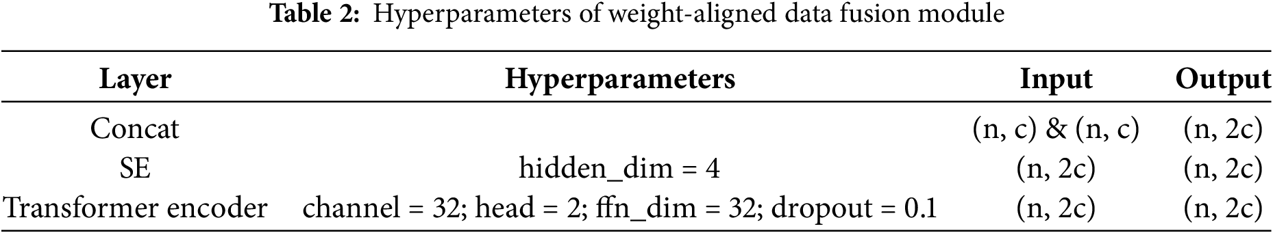
Remarks: n is the data length, c is the data dimension, hidden_dim is the dimension of the SE hidden layer, channel is the input dimension, head is the number of heads, and ffn_dim is the dimension of the FFN hidden layer.

3.3 Development of a Multi-Sensor Fusion Fault Diagnosis Model

A multi-sensor fusion fault diagnosis model is constructed using a CNN-Transformer coupled feature learning architecture and a Weight-Aligned Data Fusion Module. The specific architecture is listed in Table 3 and shown in Fig. 5.

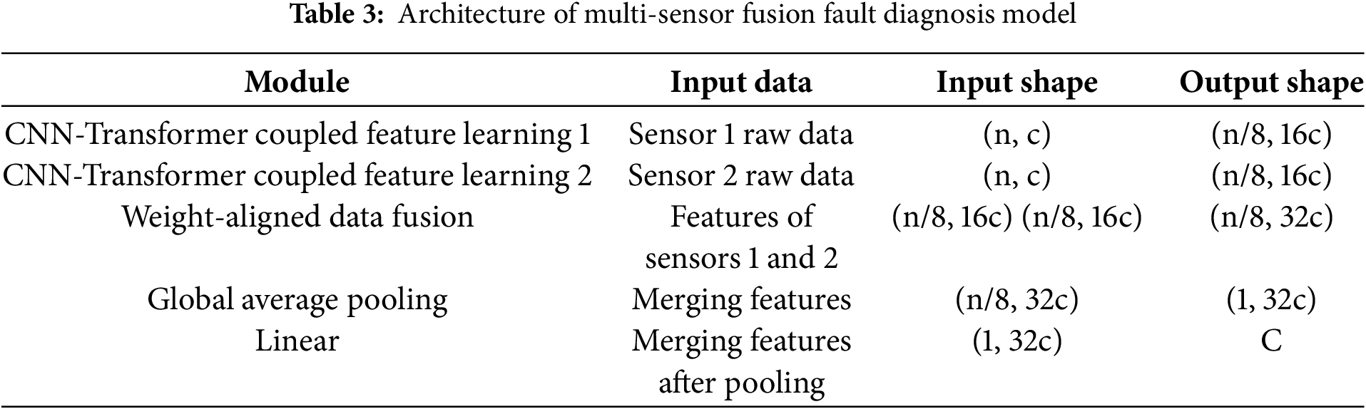
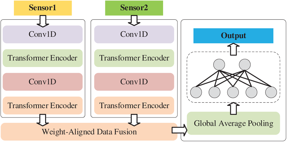
Figure 5: Architecture of multi-sensor fusion fault diagnosis model

For dual-sensor data, parallel learning is first performed through two CNN-Transformer coupled feature learning modules to obtain the corresponding features. The feature extraction modules corresponding to the two sensors do not share parameters to provide the model with richer deep-level features, enabling inference and judgment from multi-dimensional perspectives.

Next, data fusion and enhancement are performed through a Weight-Aligned Data Fusion Module. Finally, the fused features are processed through global average pooling and linear projection to obtain the output:

Output=Linear(GAP(Fo))(12)

where GAP stands for global average pooling, and Linear stands for linear layer.

Remarks: n is the data length, c is the data dimension, and C is the number of categories.

3.4 Overall Framework of the Proposed Method

This paper proposes a multi-sensor fusion-based fault diagnosis framework for wind turbine blades and applies it to noise scenarios. The overall framework of the proposed method is shown in Fig. 6. The following sections describe the proposed method step by step.

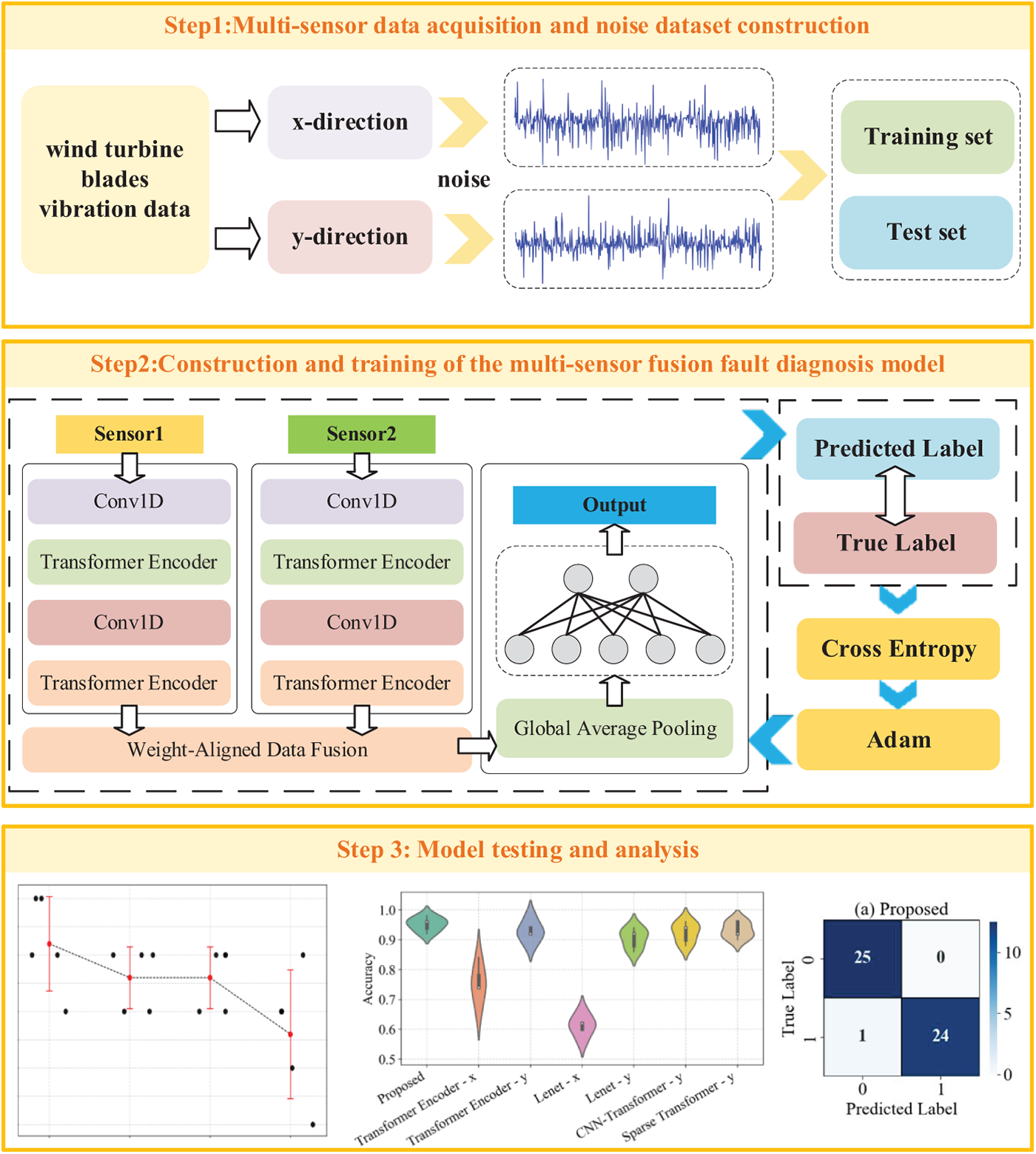
Figure 6: Overall framework of the proposed method

Step 1: Multi-sensor data acquisition and noise dataset construction. Vibration acceleration data is collected from the fan under both normal and fault conditions, and the data is divided into multiple samples. Noise is added to the samples by simulating environmental noise and sensor noise, and the samples are then divided into training and testing sets.

Step 2: Construction and training of the multi-sensor fusion fault diagnosis model. Construct a multi-sensor fusion fault diagnosis model using modules such as the CNN-Transformer coupled feature learning module and the Weight-Aligned Data Fusion Module to achieve multi-sensor data fusion and learning, ultimately enabling fault classification.

Step 3: Model testing and analysis. Quantify model performance using test set accuracy, and visualize results using scatter plots, violin plots, confusion matrices, etc.

4  Case Study

4.1 Data Introduction and Noise Dataset Establishment

The dataset analyzed in this experiment originates from the 2017 Industrial Big Data Innovation Competition, a professional event co-hosted by the China Academy of Information and Communications Technology (CAICT) and industry partners, with raw data provided by Goldwind Technology—a leading enterprise in the global wind power sector. This dataset is tailored to address a real-world industrial challenge: the prediction and diagnosis of ice accumulation faults on wind turbine blades, serving as a core resource for competitors to develop data-driven fault detection solutions. It is derived from the SCADA systems of 13 wind turbines in a specific wind farm, capturing six months of continuous operational data. Key signals included in the dataset cover critical operational and environmental parameters, such as real-time wind speed, ambient temperature, generator rotational speed, and acceleration data in two orthogonal directions (x-axis and y-axis), all structured to reflect the dynamic operating status of the wind turbines [35].

The dataset is explicitly categorized into two classes to support fault-related analysis: normal operating data and ice accumulation fault data. The temporal boundaries (start and end times) of these two operating conditions are clearly documented in two separate CSV files—normalInfo.csv for normal operation periods and failureInfo.csv for ice fault periods. For the acceleration signals (a key indicator for fault detection), sampling is performed within the time ranges defined by these two files: each sample has a fixed length of 512 data points, and no overlapping exists between consecutive samples to ensure data independence. To facilitate model training and classification, samples are labeled uniformly: normal operation samples are assigned the label “1”, while ice accumulation fault samples are labeled “2”.

To simulate a noisy environment, noise is added to the samples. The noise is randomly added Gaussian noise, whose amplitude is determined by the signal-to-noise ratio. Noise can be broadly categorized into two types: environmental noise, such as irregular vibrations caused by changes in wind speed or temperature, and vibration interference from other components like gearboxes. This type of noise typically overlays the original vibration signal and has low amplitude correlation with the original signal. Therefore, simulated environmental noise is added using the following calculation [36–38]:

y(n)add=x(n)+k⋅nstd(n)(13)

where y(n)add is a noisy signal, k is a proportional coefficient, nstd(n) is white noise, which obeys a Gaussian distribution with a mean of 0 and a variance of 1.

When determining the value of k, the signal-to-noise ratio (SNR) must be considered. SNR represents the ratio of signal power to noise power, and is usually expressed in decibels (dB) [39,40]:

SNRdB=10log10⁡(PsPn)(14)

where Ps is the power of the original signal, Pn is the power of the noise signal, and the power is calculated as follows:

Ps=1N∑n=0N−1(x(n))2(15)

The size of k can be inferred from the signal-to-noise ratio:

k=PsPn⋅10SNRdB10(16)

In addition to environmental noise, random fluctuations in sensor sensitivity can cause noise related to the amplitude of the original signal. To simulate data under sensor noise, we multiply the white noise signal by the original signal:

y(n)mul=x(n)⋅(1+k⋅nstd(n))(17)

where y(n)mul is data with simulated sensor noise added.

When adding mixed noise, add additive noise first, then add multiplicative noise, after adding noise to the samples in the corresponding manner, construct the training set and test set, with each label containing 20 training samples and 25 test samples. The training set includes an equal number of samples from each direction to ensure balanced learning of vibration characteristics. Similarly, the test set also comprises data from both directions, rather than using x-direction data exclusively for training and y-direction data for testing.

The experimental setup, environment, and operational parameters are as follows: The processor is an Intel Core i5-10400F with a base frequency of 2.90 GHz, running in an environment with Python 3.6 and TensorFlow 2.6.2. During training, we specified the Adam optimizer with a learning rate of 100, a batch size of 8, and a total of 100 training epochs. The overall experimental procedure is shown in the Fig. 7.

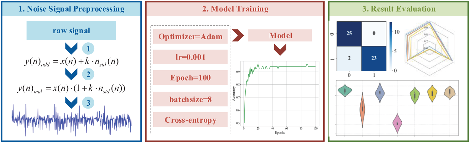
Figure 7: The overall experimental procedure

4.2 Case 1: Diagnosis of Wind Turbine Blade Fault under Simulated Environmental Noise

To simulate the effects of different environmental noises, the following experimental groups were constructed for model training and analysis, as shown in Table 4. Plot the signal diagram of acceleration in the x-direction under different noise conditions, as shown in Fig. 8.

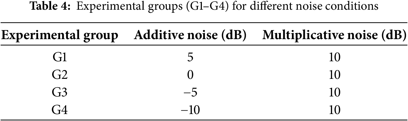
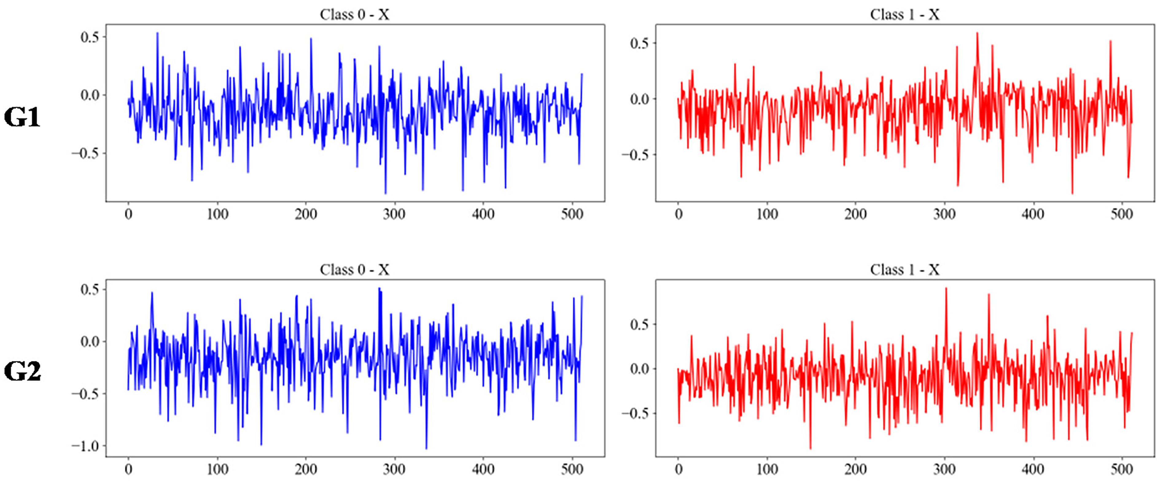
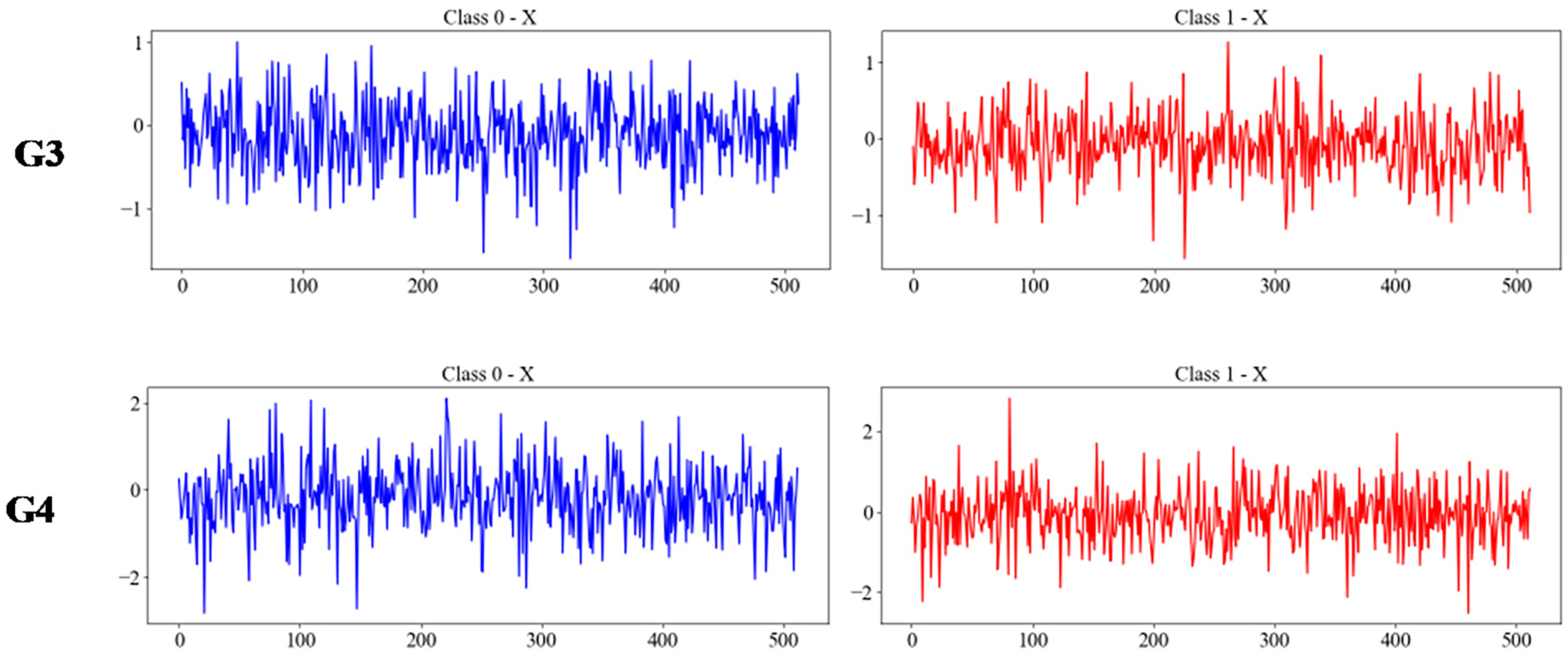
Figure 8: The acceleration signals in the x-direction under the G1–G4 experiments

The fault diagnosis model training was conducted across all experimental groups, including the Proposed method (multi-source data fusion), Transformer Encoder (single-source data input in both the x and y directions), LeNet (single-source data input in both the x and y directions) [41] and Sparse Transformer (single-source data input in y directions). In the comparison model, LeNet primarily consists of convolutional and pooling layers in a linear arrangement, aligning with the linear design of the proposed CNN-Transformer Coupled Feature Learning Architecture. The Transformer encoder consists of five layers (Since the proposed method involves computations across five Transformer Encoder layers) with two attention heads, and the hidden layer dimensions of the feedforward network are 16, 32, 32, 64, and 64, respectively. The Sparse Transformer structure is similar to the Transformer Encoder, with a window size of 8. The CNN-Transformer architecture, similar to the proposed method, adopts a single-branch structure comprising a CNN-Transformer Coupled Feature Learning module, SENet, and a fully connected layer.

To validate the effectiveness of multi-source data fusion, a model combining the key architecture of the proposed method with single-source data input (single CNN-Transformer coupled feature learning module-SE-Transformer Encoder-Classification) was also included in the experimental comparison and referred to as CNN-Transformer in subsequent experiments. Table 5 and Fig. 9 list the average accuracy rates of different methods.

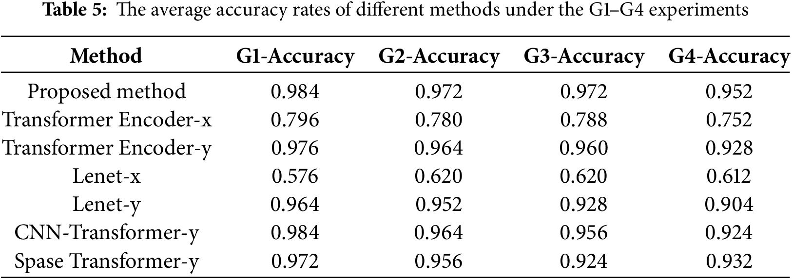
Figure 9: Radar plot of average accuracy of different methods under the G1–G4 experiments.

As shown in Table 5, the accuracy rates of the proposed method in G1–G4 are 0.984, 0.975, 0.972, and 0.952, respectively, maintaining a high overall level. As noise increases, the decline in accuracy rates is relatively gradual, demonstrating good noise robustness. The accuracy of Transformer Encoder-y decreased by approximately 0.05 in G1–G4, and the accuracy of Lenet-y decreased by approximately 0.06 in G1–G4, indicating poorer noise resistance compared to the proposed method. When compared with CNN-Transformer-y, it was found that under low-noise conditions, due to their similar structures, the diagnostic accuracy of CNN-Transformer-y is not significantly different from the proposed method. However, under strong noise conditions, its accuracy gradually falls below that of the proposed method, for example, 0.952 for the proposed method at G4 and 0.924 for CNN-Transformer-y. This indicates that multi-source data fusion can achieve complementary data features, enabling the exclusion of useless noise and the extraction of effective information under noise interference.

Table 5 shows that the diagnostic accuracy in the x-direction is relatively low, but fusing data from the x and y directions is still meaningful. The fused x-direction data can provide supplementary context, such as spatiotemporal correlations or amplitude trends that are not fully reflected in the y-direction. This helps improve the learning of y-direction features, strengthens the model’s overall feature representation, and enhances diagnostic accuracy.

Fig. 10 shows the violin plots [42] of the accuracy rates of each method in five repeated experiments on G4. The violin plot visually represents the differences in data distribution and distribution density, effectively showcasing the results of multiple experiments. From the perspective of distribution differences, the proposed method exhibits minimal distribution differences, indicating its high stability. In contrast, the accuracy differences of Transformer Encoder-x are the largest among all methods, suggesting that its results are unstable across different experiment runs on the same dataset. The proposed method maintains high accuracy even under high environmental noise conditions, demonstrating strong capabilities in extracting effective features.

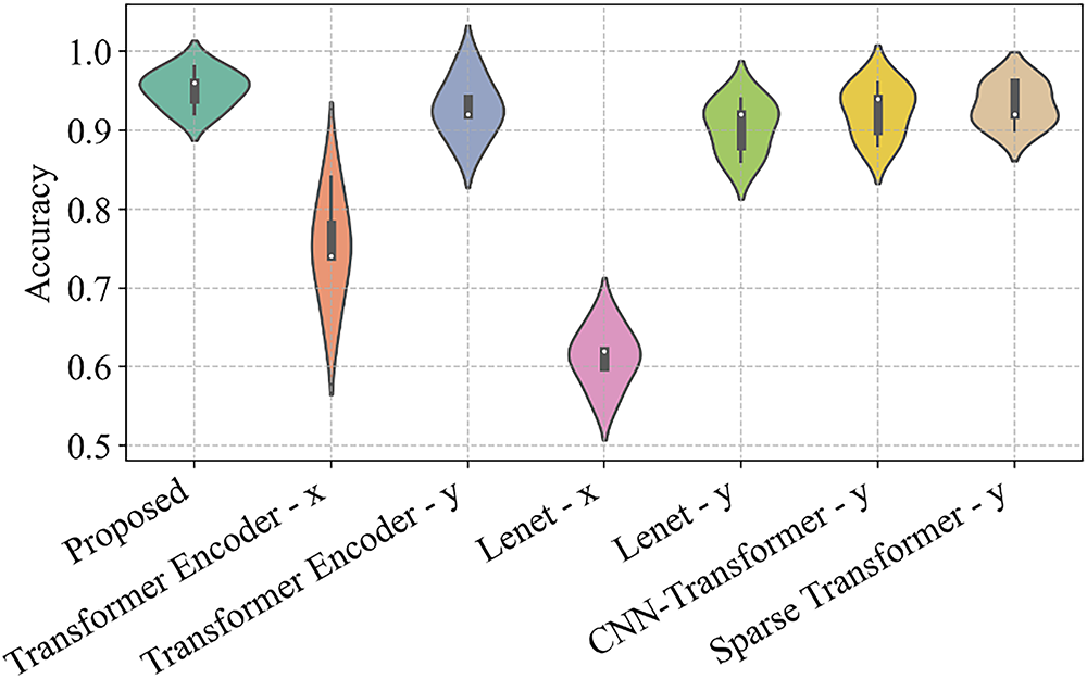
Figure 10: Violin plots of the accuracy rates of each method in five repeated runs on the G4 experiments

Fig. 11 shows the confusion matrix of the G4 experiment. The horizontal axis represents the predicted labels, and the vertical axis represents the actual labels. The confusion matrix can visualize the classification and confusion of different categories. The proposed method incorrectly predicted 1 faulty sample as a normal sample. Lenet-y incorrectly predicted 7 normal samples as faulty samples.

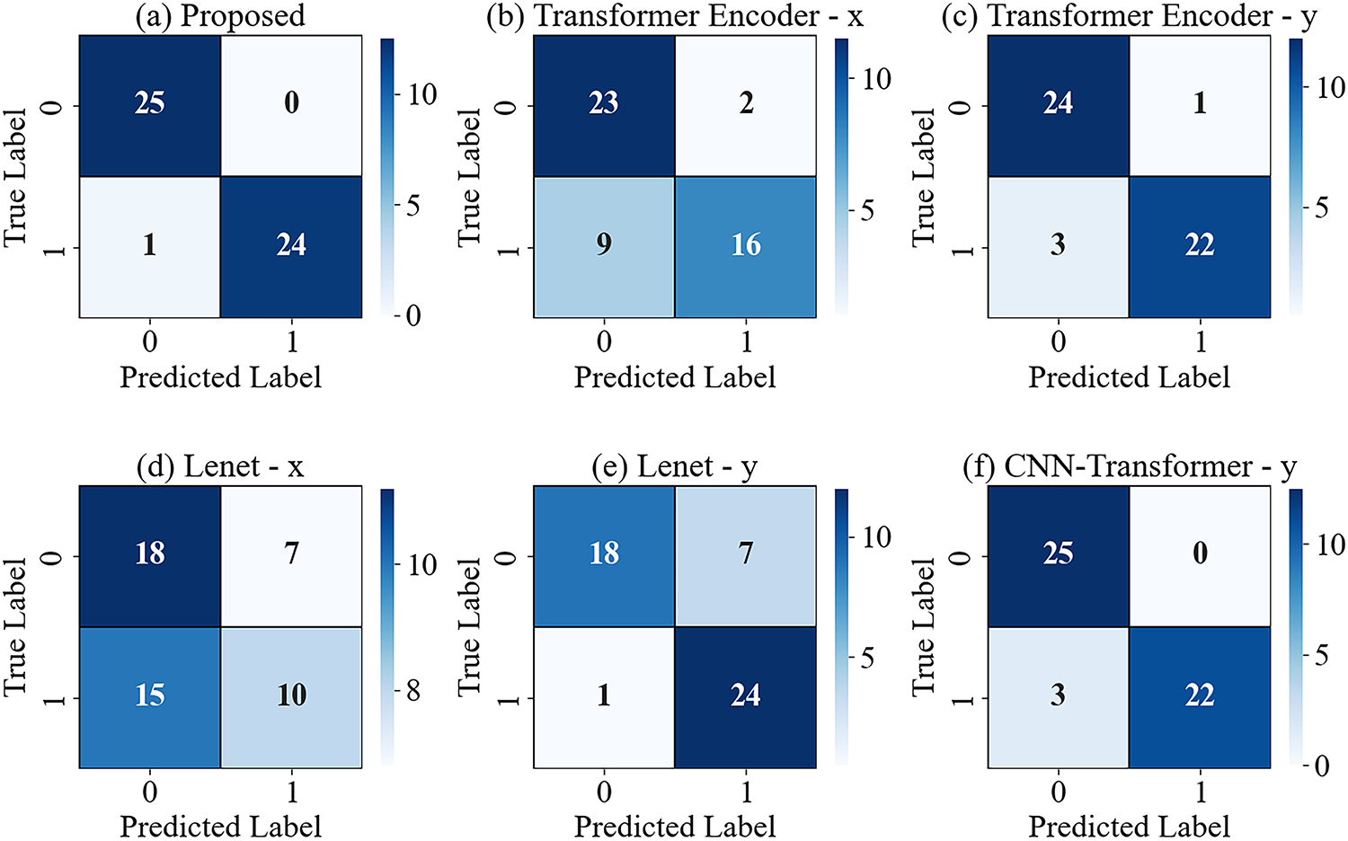
Figure 11: Confusion matrices of different methods under the G4 experiment

4.3 Case 2: Diagnosis of Wind Turbine Blade Fault under Simulated Sensor Noise

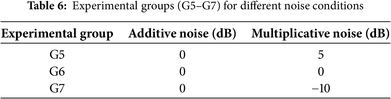
An experimental group was constructed to simulate sensor noise by adjusting the SNR of multiplicative noise. Considering the influence of sensor background noise and environmental noise on wind turbine blades during actual operation, 0 dB of additive noise was added in Case 2 to verify the model’s robustness under complex noise conditions, as shown in Table 6. Among them, the intensity of multiplicative noise increases sequentially, corresponding to a growing proportion of sensor noise.

The x and y direction signal diagrams corresponding to different groups are shown in Fig. 12. Similarly, experiments were conducted using the proposed method (multi-source data fusion), a five-layer Transformer Encoder (with single-source data input in the x and y directions, respectively), LeNet (with single-source data input in the x and y directions, respectively), and CNN-Transformer (with input in the y direction), and the average accuracy table is shown in Table 7.

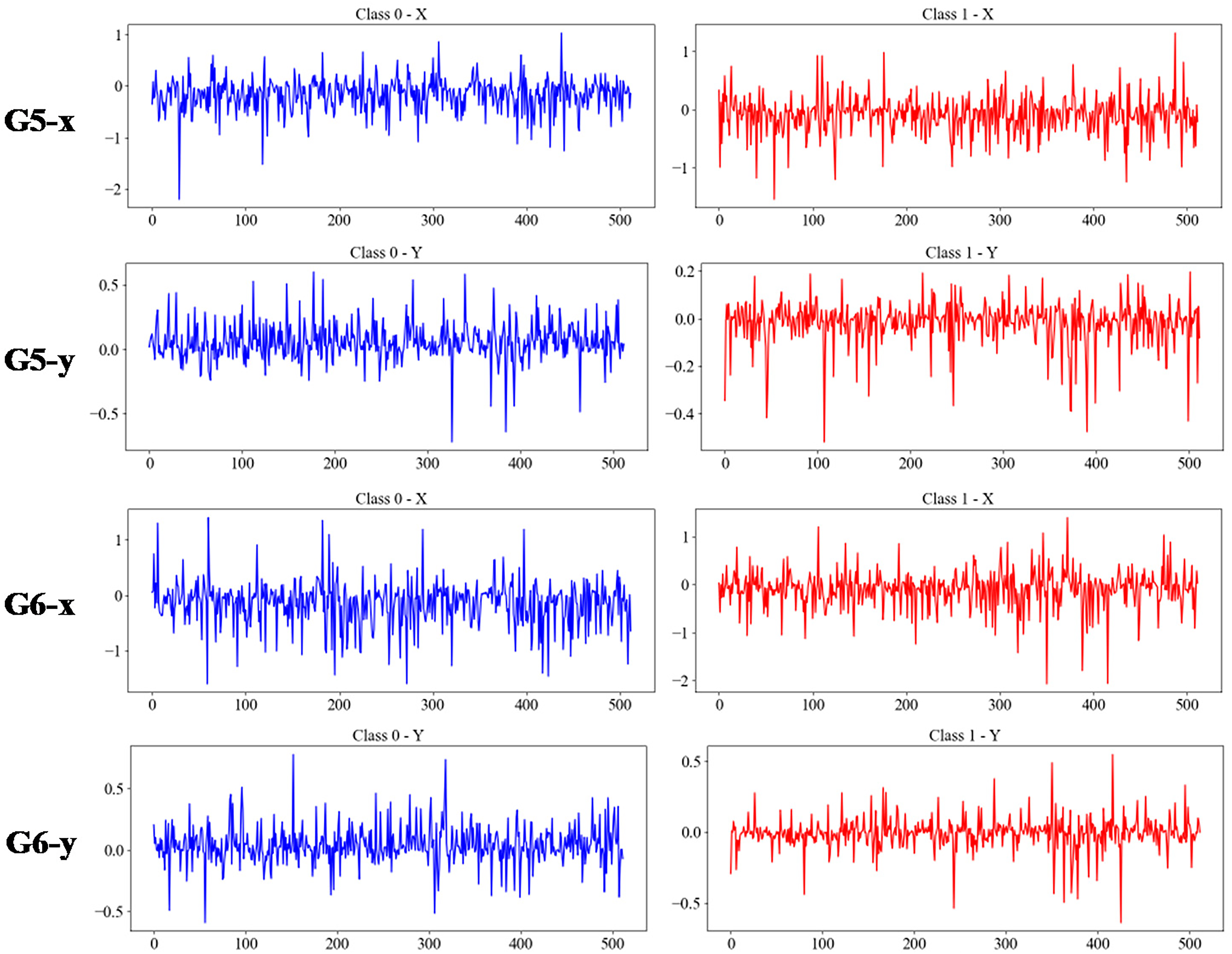
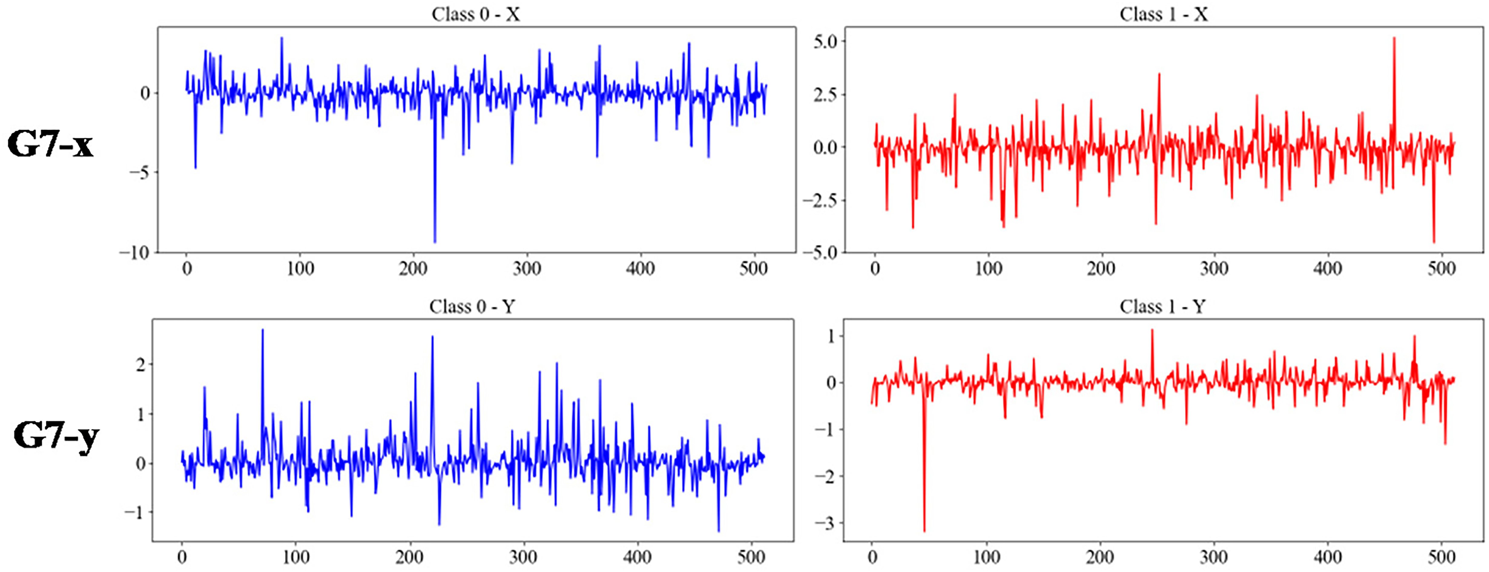
Figure 12: The acceleration signals in the x-direction and y-direction under the G5–G7 experiments

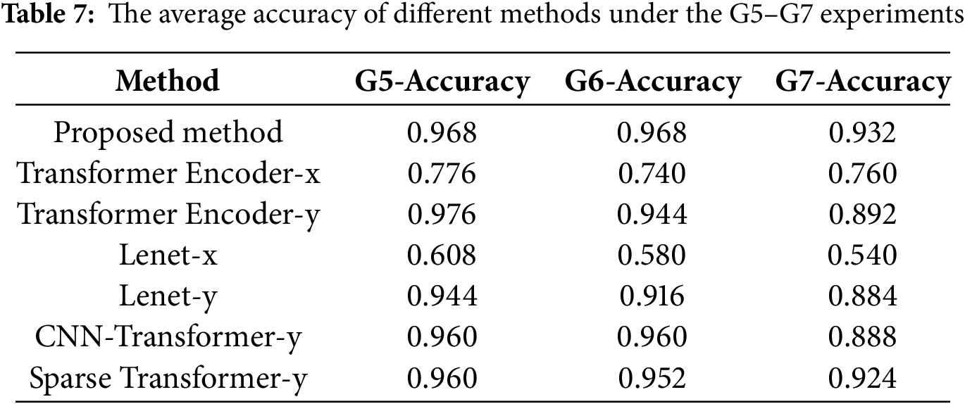
As shown in Table 7, the accuracy rates of the proposed method in G5–G7 are 0.968, 0.968, and 0.932, respectively. As the multiplicative noise increases, the accuracy rate decreases at a relatively gentle rate, demonstrating good noise robustness. Lenet-y saw a decrease of approximately 0.06 in accuracy rates for G5–G7, with poorer noise resistance compared to the proposed method. While the Transformer Encoder-x exhibits better noise resistance than the proposed method, its accuracy rates are lower than those of the proposed method. The comprehensive experimental results indicate that the proposed method can still maintain high accuracy rates under sensor noise conditions, demonstrating superior performance.

Fig. 13 shows the Training iteration curve of the proposed model on G5–G7. As dataset noise progressively increases, the training iterations of the proposed method exhibit distinct characteristics: G5 has low noise, with accuracy rapidly climbing and stabilizing at a high value with minimal fluctuation; G6 exhibits moderate noise, with accuracy increasing relatively quickly and stabilizing at a relatively steady level; G7 features high noise, resulting in a more erratic accuracy curve with significant fluctuations and slower convergence, though it ultimately achieves a high accuracy level. Overall, greater noise leads to slower convergence and poorer stability during training, yet the method still demonstrates adaptability.

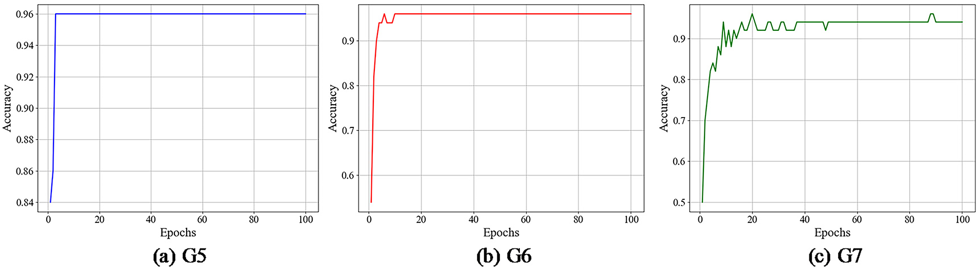
Figure 13: Training iteration curve of the proposed model on G5–G7

Fig. 14 shows the violin diagrams of different models under the G7 experiment. The proposed method can still maintain high accuracy and good stability under high sensor noise conditions, while other models, such as Lenet, show significant fluctuations in accuracy.

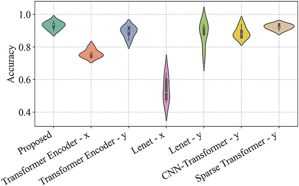
Figure 14: Violin diagrams of different methods under the G7 experiment

Fig. 15 presents the accuracy distribution of the proposed method under different experimental groups. It can be observed that the accuracy of the proposed method is not significantly affected under low-noise conditions, and only begins to decline noticeably when SNR = −10, demonstrating the method’s robust noise resistance.

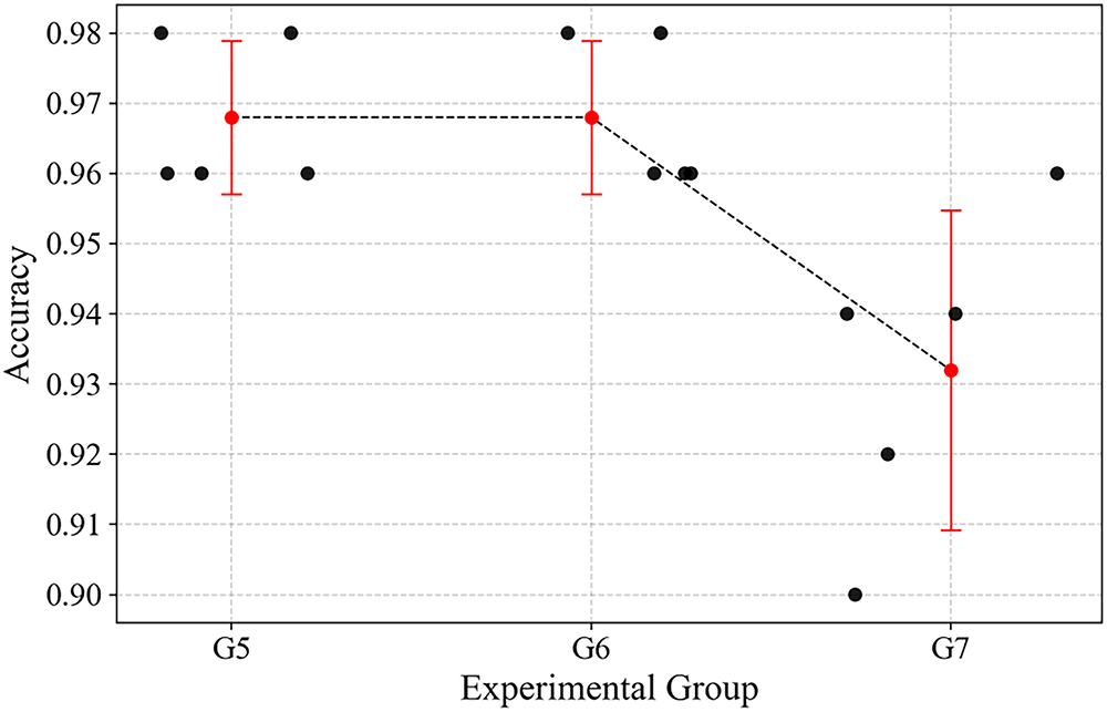
Figure 15: Accuracies of the proposed method under the G5–G7 experiments

Fig. 16 shows the confusion matrices of different methods under the G7 experiment. The proposed method incorrectly classified 2 fault samples as normal, but overall accuracy remains high. It can be observed that in high-intensity sensor noise environments, some models’ judgments are significantly disrupted. For example, Lenet-y made 6 incorrect judgments out of 50 test samples, exceeding 10%.

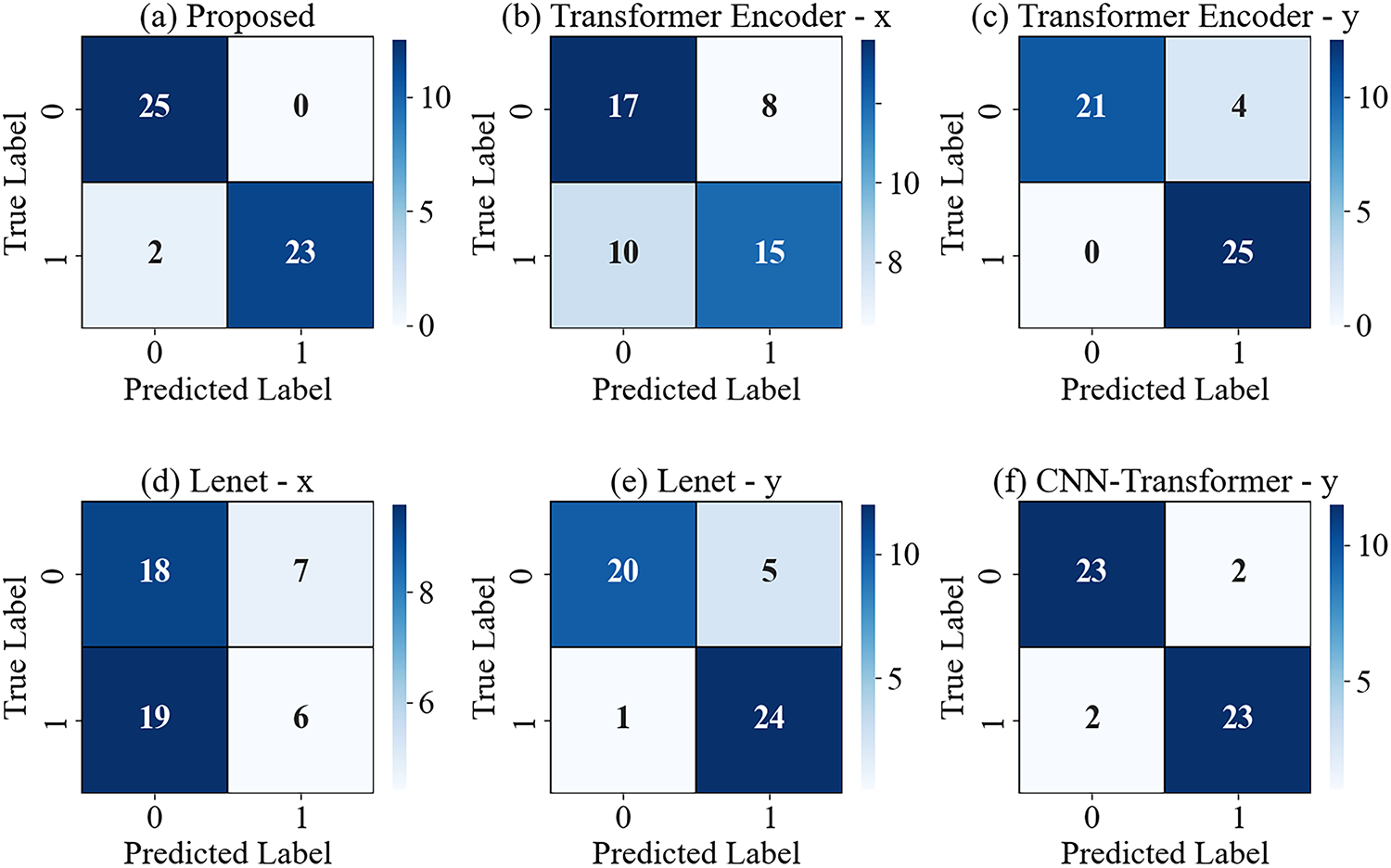
Figure 16: Confusion matrices of different methods under the G7 experiment

To validate the advantages of multi-source data input, ablation experiments were conducted. While retaining the proposed model’s CNN-Transformer Coupled Feature Learning Architecture and SENet structure, single-source data input was substituted for comparative analysis. The results are shown in Fig. 17:

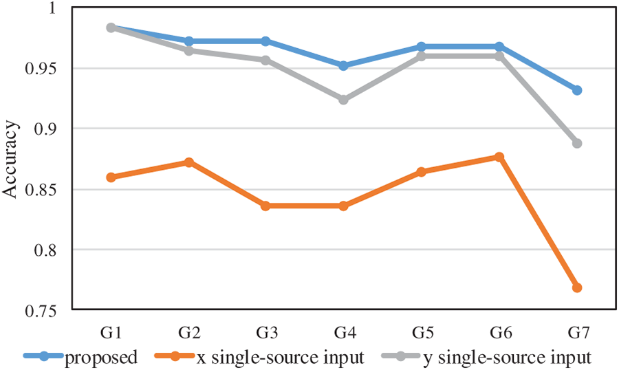
Figure 17: Accuracy curve for G1–G7 ablation experiments

The proposed method sustains relatively high accuracy across all groups from G1 to G7. In contrast, the single-source input methods exhibit more substantial performance degradation. Notably, the x single-source input experiences a sharp decline at G7. This demonstrates that the adoption of multi-source input effectively boosts the robustness and overall performance of the method in comparison to relying solely on single-source input.

5  Conclusions

This paper proposes a multi-sensor fusion method for wind turbine blade fault diagnosis. First, a Weight-Aligned Data Fusion Module is designed to comprehensively and effectively utilize multi-sensor fault information. By concatenating data from multiple sensors, weight alignment of SE units, and deep computation via the Transformer, data fusion is achieved. Second, a CNN-Transformer coupled feature learning architecture is constructed to enhance the ability to learn complex features under noisy conditions. By leveraging the complementary advantages of CNN and Transformer, the architecture balances attention to fine-grained data features with a global contextual perspective. Experimental studies were conducted under conditions simulating environmental noise and sensor noise, with multiple experimental groups designed for comparison. The results demonstrate that the proposed method effectively achieves complementary utilization of multi-sensor information, exhibits robust noise resistance. In addition, compared to traditional CNN and Transformer models, it exhibits superior feature learning capacity and diagnostic accuracy.

Beyond validating technical merits, this work underscores the potential of multi-source intelligence in advancing predictive maintenance for renewable energy assets. However, limitations remain: the method is primarily validated on a single turbine’s vibration data, and its adaptability to diverse turbine fleets or fully unstructured real-world noise profiles is not yet explored. Also, uncertainty in diagnostic outputs—which is vital for trust in industrial applications—is not addressed.

Future research will thus pursue three key avenues. First, we will extend fusion to multi-modal SCADA data (e.g., thermal, electrical signals) alongside vibration data, enabling richer cross-signal correlation. Second, we will investigate techniques to improve cross-turbine generality, such as meta-learning for rapid adaptation to new turbine designs. Third, we will integrate uncertainty-aware mechanisms (e.g., Bayesian deep learning) to quantify diagnostic confidence, ensuring safer deployment in critical wind energy operations. These efforts aim to strengthen the method’s real-world applicability and industrial impact.

Acknowledgement: We appreciate the fruitful collaboration and valuable contributions from each co-author during the research and writing process.

Funding Statement: This research is supported by the China Three Gorges Corporation (No. NBZZ202300860), the National Natural Science Foundation of China (No. 52275104), and the Science and Technology Innovation Program of Hunan Province (No. 2023RC3097).

Author Contributions: The authors confirm contribution to the paper as follows: study conception and design: Lifu He; data collection: Zhongchu Huang; analysis and interpretation of results: Haidong Shao; draft manuscript preparation: Zhangbo Hu, Yuting Wang, Jie Mei, Xiaofei Zhang. All authors reviewed the results and approved the final version of the manuscript.

Availability of Data and Materials: All datasets are publicly available.

Ethics Approval: Not applicable.

Conflicts of Interest: The authors declare no conflicts of interest to report regarding the present study.

References

1. Wang H, Shen Q, Dai Q, Gao Y, Gao J, Zhang T. Evolutionary variational YOLOv8 network for fault detection in wind turbines. Comput Mater Contin. 2024;80(1):625–42. doi:10.32604/cmc.2024.051757. [Google Scholar] [CrossRef]

2. Baliatsas C, Yzermans CJ, Hooiveld M, Kenens R, Spreeuwenberg P, van Kamp I, et al. Health problems near wind turbines: a nationwide epidemiological study based on primary healthcare data. Renew Sustain Energy Rev. 2025;216(3):115642. doi:10.1016/j.rser.2025.115642. [Google Scholar] [CrossRef]

3. Kang S, He Y, Li W, Liu S. Research on defect detection of wind turbine blades based on morphology and improved otsu algorithm using infrared images. Comput Mater Contin. 2024;81(1):933–49. doi:10.32604/cmc.2024.056614. [Google Scholar] [CrossRef]

4. Marouani H, Awjah Almehmadi F, Farkh R, Dhahri H. Wind turbine efficiency under altitude consideration using an improved particle swarm framework. Comput Mater Contin. 2022;73(3):4981–94. doi:10.32604/cmc.2022.029315. [Google Scholar] [CrossRef]

5. Lai Z, Liu Y, Cai J, Cheng X, Liu X. FreqICE: efficient blade icing detection on wind turbines via frequency learning. IEEE Sens J. 2025;25(8):14005–13. doi:10.1109/JSEN.2025.3547698. [Google Scholar] [CrossRef]

6. Xiong S, Zhou H, He S, Zhang L, Shi T. Fault diagnosis of a rolling bearing based on the wavelet packet transform and a deep residual network with lightweight multi-branch structure. Meas Sci Technol. 2021;32(8):085106. doi:10.1088/1361-6501/abe448. [Google Scholar] [CrossRef]

7. Yan M, Hui SC, Jiang N, Li N. A review on data-driven prognostics and health management for wind turbine systems. Eng Appl Artif Intell. 2025;159(2):111484. doi:10.1016/j.engappai.2025.111484. [Google Scholar] [CrossRef]

8. Gao W, Liu J, Cui C, Liu X, Fang Y. An efficient image stitching method of wind-turbine blades for damage measurement in online repair robots. Measurement. 2025;256:118125. doi:10.1016/j.measurement.2025.118125. [Google Scholar] [CrossRef]

9. Zhang D, Zhao T, Wang B, Xu H, Hua Y, Shi S, et al. Structural health monitoring on operating offshore wind turbine blade via a single accelerometer: feasibility study by simulation and experiment. Measurement. 2025;244:116432. doi:10.1016/j.measurement.2024.116432. [Google Scholar] [CrossRef]

10. Ying L, Xu Z, Zhang H, Xu J, Cheng X. Graph temporal attention network for imbalanced wind turbine blade icing prediction. IEEE Sens J. 2024;24(6):9187–96. doi:10.1109/JSEN.2024.3358873. [Google Scholar] [CrossRef]

11. Wu W, Zhou N, Liang X, Gui W, Yang C, Liu Y. TCAC-transformer: a fast convolutional transformer with temporal-channel attention for efficient industrial fault diagnosis. Expert Syst Appl. 2026;297(2):129473. doi:10.1016/j.eswa.2025.129473. [Google Scholar] [CrossRef]

12. Liu K, Li Y, Cui Z, Qi G, Wang B. Adaptive frequency attention-based interpretable Transformer network for few-shot fault diagnosis of rolling bearings. Reliab Eng Syst Saf. 2025;263(24):111271. doi:10.1016/j.ress.2025.111271. [Google Scholar] [CrossRef]

13. Wei C, Cai S, Yang H, Zhang Y. Advanced deep learning-based methodology for multi-class diagnosis of wind turbine blade faults at the wind farm level. Eng Appl Artif Intell. 2025;160(1):111801. doi:10.1016/j.engappai.2025.111801. [Google Scholar] [CrossRef]

14. Sethi MR, Subba AB, Faisal M, Sahoo S, Koteswara Raju D. Fault diagnosis of wind turbine blades with continuous wavelet transform based deep learning model using vibration signal. Eng Appl Artif Intell. 2024;138:109372. doi:10.1016/j.engappai.2024.109372. [Google Scholar] [CrossRef]

15. Pan X, Chen A, Zhang C, Wang J, Zhou J, Xu W. Wind turbine blade fault detection based on graph Fourier transform and deep learning. Digit Signal Process. 2025;159(15):105007. doi:10.1016/j.dsp.2025.105007. [Google Scholar] [CrossRef]

16. Guo J, Liu C, Liu S, Liu W. Graph contrastive learning for semi-supervised wind turbine fault diagnosis with few labeled SCADA data. Measurement. 2025;245(7):116531. doi:10.1016/j.measurement.2024.116531. [Google Scholar] [CrossRef]

17. Yan H, Zhou H, Zheng J, Zhou Z. Rolling bearing fault diagnosis based on 1D convolutional neural network and Kolmogorov-Arnold network for industrial Internet. Comput Mater Contin. 2025;83(3):4659–77. doi:10.32604/cmc.2025.062807. [Google Scholar] [CrossRef]

18. Liu X, Zhang Z. A two-stage deep autoencoder-based missing data imputation method for wind farm SCADA data. IEEE Sens J. 2021;21(9):10933–45. doi:10.1109/JSEN.2021.3061109. [Google Scholar] [CrossRef]

19. Hao N, Chen T, Jia R, Wang L. Fault diagnosis method for vehicle transmission system’s spindle bearing based on double-discriminator GAN and conv-KAN model. Meas Sci Technol. 2025;2025(8):085115. doi:10.1088/1361-6501/adf084. [Google Scholar] [CrossRef]

20. Wu C, Zheng S. Fault diagnosis method of rolling bearing based on MSCNN-LSTM. Comput Mater Contin. 2024;79(3):4395–411. doi:10.32604/cmc.2024.049665. [Google Scholar] [CrossRef]

21. Lv Y, Hao J, Tang M, Wu J. Multimodal data fusion-based intelligent fault diagnosis for ship rotating machinery: status quo and perspectives. Eng Appl Artif Intell. 2025;160(6):111767. doi:10.1016/j.engappai.2025.111767. [Google Scholar] [CrossRef]

22. Ma L, Yang Q, Llanes-Santiago O, Peng K. A multi-source heterogeneous data fusion framework for fault diagnosis in industrial processes with missing image data. Measurement. 2025;256(3):118278. doi:10.1016/j.measurement.2025.118278. [Google Scholar] [CrossRef]

23. Zhang H, Li Y, Zhang X, Feng H. Multi-scale group Mamba network with structural attention for rotating machinery fault diagnosis using multisensor data. Adv Eng Inform. 2025;67(6):103521. doi:10.1016/j.aei.2025.103521. [Google Scholar] [CrossRef]

24. Lai Z, Cheng X, Liu X, Huang L, Liu Y. Multiscale wavelet-driven graph convolutional network for blade icing detection of wind turbines. IEEE Sens J. 2022;22(22):21974–85. doi:10.1109/JSEN.2022.3211079. [Google Scholar] [CrossRef]

25. Hu X, Wei D, Liu D, Xiao Z, Xia X, Malik OP. Fault diagnosis for rotor based on multi-sensor information and progressive strategies. Meas Sci Technol. 2023;34(6):065111. doi:10.1088/1361-6501/acc11c. [Google Scholar] [CrossRef]

26. He C, Hao R, Yang K, Yuan Z, Sang S, Wang X. Bearing fault diagnosis with DDCNN based on intelligent feature fusion strategy in strong noise. Comput Mater Contin. 2023;77(3):3423–42. doi:10.32604/cmc.2023.045718. [Google Scholar] [CrossRef]

27. Liu R, Zhang L, Jia J, Li S, Guo H, Guo B. A 1DCNN-SENet-LSTM model for UGW-based automatic evaluation of grouting void location in post-tensioned concrete structure. Eng Struct. 2025;339(2):120669. doi:10.1016/j.engstruct.2025.120669. [Google Scholar] [CrossRef]

28. Han T, Wang X, Guo J, Chang Z, Chen Y. Health-aware joint learning of scale distribution and compact representation for unsupervised anomaly detection in photovoltaic systems. IEEE Trans Instrum Meas. 2025;74:3538811. doi:10.1109/TIM.2025.3571122. [Google Scholar] [CrossRef]

29. Vaswani A, Shazeer N, Parmar N, Uszkoreit J, Jones L, Gomez AN, et al. Attention is all you need. arXiv: 1706.03762. 2017. [Google Scholar]

30. Yang X, She Y, Li Y, Luo M. A signal is worth 8 words: coal mine mechanical fault diagnosis with transformers. In: 2025 IEEE 14th Data Driven Control and Learning Systems (DDCLS); 2025 May 9–11; Wuxi, China: IEEE; 2025. p. 1316–21. doi:10.1109/DDCLS66240.2025.11065775. [Google Scholar] [CrossRef]

31. Wan B, Jiang W, Fang Y, Wen W, Liu H. Dual-stream self-attention network for image captioning. In: 2022 IEEE International Conference on Visual Communications and Image Processing (VCIP); 2022 Dec 13–16; Suzhou, China: IEEE; 2022. p. 1–5. doi:10.1109/VCIP56404.2022.10008904. [Google Scholar] [CrossRef]

32. Yan X, Zhang H, Di Y, Xie L. Research on IoT sensor data correlation and anomaly detection based on self-attention mechanisms. In: 2025 5th International Conference on Consumer Electronics and Computer Engineering (ICCECE); 2025 Feb 28–Mar 2; Dongguan, China: IEEE; 2025. p. 802–5. doi:10.1109/ICCECE65250.2025.10985672. [Google Scholar] [CrossRef]

33. Zhang X, Wen C. Fault diagnosis of rolling bearings based on dual-channel Transformer and Swin Transformer V2. In: 2024 43rd Chinese Control Conference (CCC); 2024 Jul 28–31; Kunming, China: IEEE; 2024. p. 4828–34. [Google Scholar]

34. Hu J, Shen L, Sun G. Squeeze-and-excitation networks. In: 2018 IEEE/CVF Conference on Computer Vision and Pattern Recognition; 2018 Jun 18–23; Salt Lake City, UT, USA: IEEE; 2018. p. 7132–41. doi:10.1109/CVPR.2018.00745. [Google Scholar] [CrossRef]

35. Liu Y, Cheng H, Kong X, Wang Q, Cui H. Intelligent wind turbine blade icing detection using supervisory control and data acquisition data and ensemble deep learning. Energy Sci Eng. 2019;7(6):2633–45. doi:10.1002/ese3.449. [Google Scholar] [CrossRef]

36. Yang L, Cao L, Wang J, Yao X, Shen Y, Wu Y. Bearing fault feature extraction measure using multi-layer noise reduction technology. In: 2022 IEEE International Conference on Sensing, Diagnostics, Prognostics, and Control (SDPC); 2022 Aug 5–7; Chongqing, China: IEEE; 2022. p. 53–6. doi:10.1109/SDPC55702.2022.9915997. [Google Scholar] [CrossRef]

37. Chen W, Mao R, Gong B, Fang M, Yang Z, Li Y. A fault diagnosis method for Railway Point Machines based on imbalanced data under natural noise environment. Measurement. 2026;257(4):118543. doi:10.1016/j.measurement.2025.118543. [Google Scholar] [CrossRef]

38. Yu Z, Gao S, Zhao W, He B. Noise-robust underwater propeller fault diagnosis through dictionary learning and graph convolutional networks. Ocean Eng. 2025;339(4):122166. doi:10.1016/j.oceaneng.2025.122166. [Google Scholar] [CrossRef]

39. Li Y, Huang X, Yu S, Kumar M, Peng S. Temporal-mask multiple-scale fusion network: a novel hybrid network framework for robust fault diagnosis under varying noise interference. Comput Chem Eng. 2025;202:109327. doi:10.1016/j.compchemeng.2025.109327. [Google Scholar] [CrossRef]

40. Zhang Y, Zhao X, Peng Z, Xu R, Chen P. WD-KANTF: an interpretable intelligent fault diagnosis framework for rotating machinery under noise environments and small sample conditions. Adv Eng Inform. 2025;66(6):103452. doi:10.1016/j.aei.2025.103452. [Google Scholar] [CrossRef]

41. Yan C, Li J. Hydrogen leakage diagnosis of fuel cell vehicles based on a dynamic-static recognition approach with dual-channel LeNet network. Fuel. 2023;352(9):128936. doi:10.1016/j.fuel.2023.128936. [Google Scholar] [CrossRef]

42. Xiao Y, Shao H, Liu B. Evaluating calibration of deep fault diagnostic models under distribution shift. Comput Ind. 2025;171:104334. [Google Scholar]