Adaptive Learned Index Construction with Sliding Windows for High-Throughput Blockchain Systems

1  Introduction

In recent years, the rapid development of distributed energy technologies and the diversified transformation of energy market demands have driven the innovation and upgrading of electricity trading forms. Traditional centralized electricity trading systems, struggling to meet modern energy market requirements for flexibility and responsiveness, are accelerating their transition toward distributed architectures and intelligent models. During this transformation, electricity trading systems must not only enhance compatibility with distributed energy integration and adaptability to market dynamics but also address multiple challenges such as trustworthy data management, transaction security, and system operational reliability. Notably, blockchain technology, characterized by decentralization, traceability, and tamper resistance, has been widely recognized as a trustworthy infrastructure for distributed systems and secure transaction management [1]: its distributed ledger technology effectively supports peer-to-peer electricity trading [2], smart contracts ensure transparent and trustworthy transaction processes, asymmetric encryption algorithms provide technical safeguards for power data privacy [3], and consensus mechanisms defend against false data injection attacks [4], thereby establishing a secure and reliable electricity trading ecosystem.

Despite blockchain’s decentralized trust mechanisms, its data storage architecture faces inherent constraints. Whether using linear chain structures or Directed Acyclic Graph (DAG)-based blockchain systems, all adhere to an append-only data persistence model. As electricity trading frequency evolves to minute- or even second-level intervals, blockchain ledger data grows superlinearly. In this context, traditional B+ tree-based indexing solutions encounter dual bottlenecks: (1) storage space inflation leading to exponential operational costs, and (2) lack of data locality causing random query latency spikes. This systemic imbalance between storage and query performance creates performance ceilings for blockchain in real-time electricity settlement and high-frequency demand response bidding scenarios.

Current research on blockchain query optimization focuses on two directions: on-chain and off-chain optimizations. For on-chain improvements, studies aim to enhance intra-block data structures. While block data is typically stored as Merkle trees for efficient existence verification, full nodes must traverse entire blocks to retrieve specific information, resulting in low query efficiency. Li et al. [5] proposed an efficient and verifiable index management system for blockchain dynamic queries (FlexIM) that leverages authenticated indexing structures to support rapid transaction localization while reducing unnecessary block traversal. Jia et al. [6] designed the B-M tree, constructing a balanced binary tree based on user addresses and filtering blocks by recording leaf node address ranges. Zhang and Wei [7] developed a trie-linked list hybrid index, leveraging public keys for trie-based navigation and grouped transaction storage. Liu et al. [8] embedded Bloom filters in non-leaf Merkle tree nodes to reduce invalid traversals by pre-judging transaction existence. Wang et al. [9] introduced a multi-level index for master-slave blockchains, using jump-consistent hashing for the main chain and enhanced Bloom filters for side chains, effectively reducing cross-chain query overhead. However, these methods still require backward traversal from the latest block, leading to significant redundant searches for deep-block targets [10], while structural complexity limits practical scalability.

For off-chain optimizations, Wu et al. [11] proposed a micro-database middleware layer to extract and query blockchain data in real time. Muzammal et al. [12] integrated blockchain systems with distributed databases to enable efficient off-chain query processing while preserving data integrity and synchronization. A blockchain database application platform (ChainSQL) combined blockchain with distributed databases to ensure tamper-proof data and fast query responses. Xie et al. [13] split blockchain data into index and transaction databases for rapid retrieval. However, as blockchain data scales, off-chain databases face declining update and query efficiency, while also incurring increased tampering risks and storage burdens.

Beyond query and indexing efficiency, blockchain-based data management systems should explicitly consider data privacy. Searchable symmetric encryption (SSE) combined with smart contracts has been widely adopted for privacy-preserving data sharing, where both data and queries are processed on-chain in encrypted form. However, naively extending single-keyword search to multi-keyword queries may expose intermediate results to blockchain nodes and incur substantial computational and monetary overhead. Jiang et al. [14] addressed these issues with a Bloom-filter-based multi-keyword search protocol: it first filters the database using low-frequency keywords and then completes the search in a single round via pseudorandom labels, thereby reducing intermediate leakage and improving efficiency. Their evaluation shows reduced query latency and significantly lower on-chain cost, indicating that privacy protection can (and should) be co-designed with system efficiency optimization. Our learned index focuses on optimizing the timestamp-to-block-height mapping at the index (metadata) layer rather than operating on raw transaction contents; thus, it is complementary to existing privacy-preserving techniques and can be integrated seamlessly to support secure and efficient blockchain query processing.

The convergence of blockchain technology with the Internet of Things (IoT), particularly in Industrial IoT (IIoT) environments, introduces stringent requirements on transaction throughput, latency, and security. In such settings, a large number of heterogeneous devices continuously generate time-sensitive data, which must be securely recorded, validated, and retrieved with minimal delay. Permissioned blockchain architectures are therefore widely adopted in IoT-enabled systems, as they provide controlled access, identity verification, and enhanced privacy while maintaining a certain level of decentralization. However, the effectiveness of these systems is largely constrained by the efficiency of their consensus and execution mechanisms, especially under high-frequency transactional workloads.

Ayub Khan et al. [15] addressed these challenges by proposing a blockchain-oriented lightweight Proof-of-Elapsed-Time (B-LPoET), a lightweight middleware-based enhancement to the Proof-of-Elapsed Time consensus mechanism, which leverages multithreading and optimized execution scheduling to reduce block generation latency and improve transaction throughput in permissioned blockchain environments, making it particularly suitable for IoT-enabled and enterprise-oriented blockchain systems. Within this context, lightweight middleware-based enhancements to Proof-of-Elapsed Time (PoET), such as B-LPoET, provide an important system-level advancement for IoT–blockchain integration. By incorporating multithreading and optimized execution scheduling, such approaches significantly reduce block generation time and improve transaction throughput without sacrificing security guarantees. This is particularly beneficial for IoT-enabled enterprise environments, where timely data confirmation and scalable execution are critical for applications such as smart manufacturing, energy management, and distributed control systems. Overall, efficient consensus execution and fast block indexing mechanisms—such as the proposed SW-LI—are essential enablers for realizing robust, secure, and high-performance blockchain infrastructures tailored to IoT ecosystems.

Existing public-chain-oriented consensus algorithms, such as Proof-of-Work and Proof-of-Stake, are generally unsuitable for IoT scenarios due to their high computational overhead and energy consumption. Practical Byzantine Fault Tolerance and Raft-based mechanisms, although more common in permissioned environments, suffer from scalability limitations and increased communication costs as the number of participating nodes grows. In contrast, PoET has emerged as a promising alternative for private IoT-driven blockchains by reducing communication overhead and enabling fair leader selection through randomized waiting times. Nevertheless, traditional PoET implementations rely heavily on trusted execution environments and exhibit limited flexibility in handling dynamic workloads and parallel transaction execution.

To address the limitations of B+ trees in space efficiency and query performance, learned indexes leveraging machine learning for key-value mapping have shown promise. Literature [16] applied piecewise linear regression in the DAG-based blockchain Conflux, mapping timestamps to epoch intervals and combining aggregated Bloom filters for cross-epoch queries. Literature [17] dynamically built inter-block indexes using incremental methods with error-bound-based linear segmentation. Literature [18] employed online gradient descent and sliding window search to parameterize timestamp-to-block-height mappings, but query latency spikes under irregular data distributions. Existing learned indexes face two limitations: (1) Single-segment linear regression is prone to error accumulation during abrupt data changes, and (2) Point-wise construction methods suffer from low computational efficiency and interference from historical data.

Building on these works, this paper proposes SW-LI, a sliding window-based learned index construction method for blockchain timestamp-to-block-height mapping. SW-LI enhances index construction efficiency while reducing block traversal during queries, significantly improving performance in large-scale scenarios. Key contributions include: (1) sliding window-based data selection and linear regression modeling for timestamp-height mapping, and (2) a dynamic window adjustment mechanism that shrinks window spans when prediction errors exceed thresholds to improve local accuracy or expands windows to accelerate global indexing. Experiments show that as block counts grow from 5000 to 25,000, SW-LI achieves 69.22%–88.22% higher construction efficiency than Anole. At 10,000 blocks, SW-LI reduces prediction errors by 80% compared to SWS-OGD, with only 60 KB storage overhead (25,000 blocks), validating its superior efficiency and precision.

Based on the aforementioned research, this paper proposes SW-LI (Sliding Window-based Learned Index), an adaptive learned index construction method for blockchain systems, aiming to efficiently establish dynamic mappings between block timestamps and block heights. The core contributions of this study are as follows:

(1) Lightweight Sliding Window-Regression Joint Modeling Mechanism

A sliding window-driven data selection strategy is proposed, where localized timestamp-height samples are used to train linear regression models for lightweight block positioning. Each window only stores slope and intercept parameters. Compared to traditional point-wise index construction methods, the window-based batch processing mechanism reduces the computational complexity from O(n) to O(n/w) (where w is the average window size), significantly mitigating interference from historical data.

(2) Error-Feedback-Driven Dynamic Window Adjustment Algorithm

To address the limitations of traditional learned indexes in dynamic data scenarios, a dual-layer adaptive window adjustment mechanism is proposed:

•   When the maximum prediction error within a window exceeds a preset threshold ε, the window span is halved and the local data is refitted to suppress error accumulation caused by abrupt changes in block generation rates or local nonlinearity.

•   Conversely, if the error remains below ε, the window span is incrementally expanded to cover more linearly distributed regions, reducing the number of index segments and improving global construction efficiency.

(3) Performance Verification for High-Throughput Blockchains

Experiments based on real Ethereum transaction datasets demonstrate the exceptional performance of the SW-LI method in high-throughput blockchain scenarios:

•   As the number of blocks increases from 5000 to 25,000, its index construction efficiency improves by 69.22%–88.22% compared to Anole, while storage overhead remains stable at 60 KB.

•   At a scale of 10,000 blocks, its prediction error is reduced by an average of 80% compared to SWS-OGD.

•   When a block contains 4000 transactions, the average total query latency of SW-LI is 46.15% lower than Anole and amounts to just 2.7% of the average query latency of SWS-OGD (i.e., approximately 37 times faster).

This method provides a theoretically rigorous and practically feasible solution for real-time query optimization in high-throughput blockchain systems.

2  System Model

In the blockchain system, each node maintains a learned index to facilitate efficient data retrieval. When a node receives a query request containing a timestamp attribute, it leverages the learned index to rapidly identify the segment interval to which the timestamp belongs. It then retrieves the linear regression parameters associated with that segment. Using these parameters, the node predicts the approximate block height corresponding to the target timestamp. Starting from the predicted block height, the system performs a localized search within neighboring blocks to accurately determine the actual block height containing the timestamp and the corresponding transaction. The overall process of learned index construction and timestamp-based query execution is illustrated in Fig. 1.

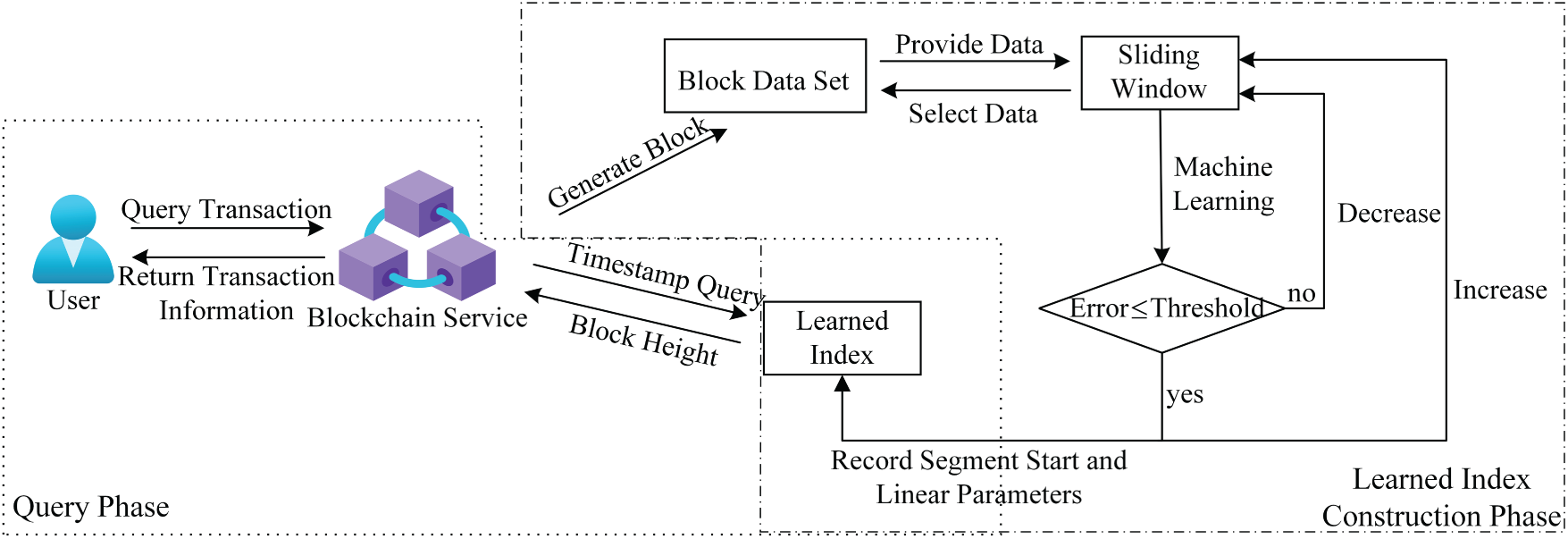
Figure 1: Overview of the SW-LI index construction and querying process.

3  Adaptive Learning Index Based on Sliding Window

3.1 Learning Index Construction Process

In blockchain systems, blocks are generated by nodes through consensus protocols. Whenever a node produces a new block or receives a synchronized block from its peers, it extracts the corresponding block timestamp and block height and appends them to a cumulative dataset. For clarity, Nomenclature section summarizes the key symbols, variables, and abbreviations used in the following sections.

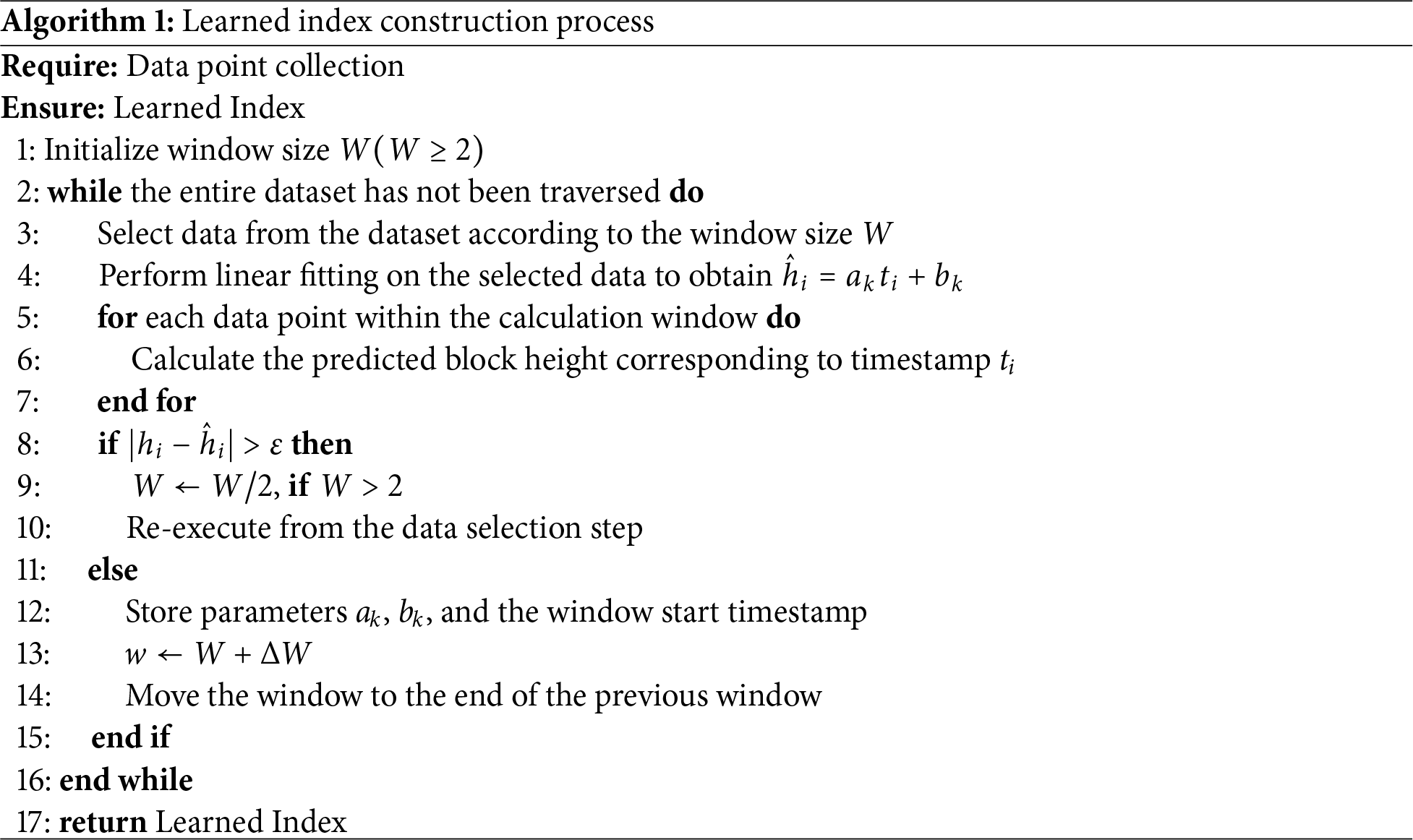
To construct the learned index, we initialize a sliding window of size W (W≥2) and slide it sequentially over the dataset. We adopt W=2 as the minimal initialization size for linear fitting, which mainly affects cold-start overhead because the window is resized adaptively thereafter. At the k-th window position, we collect W timestamp–height pairs, denoted as

𝒟k={(ti,hi)}i=kk+W−1.(1)

Based on these samples, we fit a linear regression model using the least squares method, which establishes a mapping from timestamps to block heights. The predicted block height is expressed as

h^i=akti+bk,(2)

where ak and bk are the slope and intercept parameters of the k-th window, respectively, obtained by minimizing the squared residuals within the window.

ak,bk=arg⁡mina,b∑i=kk+W−1[hi−(ati+b)]2(3)

The solution process is as follows. First, construct the matrices:

A=[tk1tk+11⋮⋮tk+W−11],H=[hkhk+1⋮hk+W−1](4)

Let the parameter vector C=[akbk]T. The optimal solution can be obtained by solving the normal equation:

ATAC=ATH(5)

Solving this yields:

C=(ATA)−1ATH(6)

Using the obtained coefficient vector C, the predicted height h^i for each data point in the window can be computed as:

h^i=akti+bk.(7)

To improve numerical stability and comparability across windows, we apply Z-score normalization to both timestamps and block heights within each window. For the k-th window, we compute the mean and standard deviation and normalize each value accordingly. Because these statistics are computed locally, the normalization adapts to the window’s data distribution and mitigates fluctuations caused by non-stationary block generation intervals. This, in turn, improves the fitting quality of the linear model under dynamic blockchain conditions.

First, compute the arithmetic mean μk of all timestamps within the k-th sliding window,

μk=1W∑i=kk+W−1ti.(8)

where ti denotes the i-th timestamp in the time series, N is the total number of timestamps, and W is the sliding window size.

Next, calculate the standard deviation σk of all timestamps within the k-th sliding window based on the computed arithmetic mean,

σk=1W∑i=kk+W−1(ti−μk)2.(9)

Finally, normalize the timestamps using the computed arithmetic mean μk and standard deviation σk,

ti=ti′−μkσk.(10)

To distinguish between normalized timestamps and timestamps within the window, we use ti to denote normalized timestamp data and t′ to denote timestamp data within the window.

The process of standardizing block height follows the same procedure as standardizing timestamps. First, the mean value of block height μh is calculated as follows:

μh=1n∑j=1nhj.(11)

where hj denotes the j-th block height in the sequence, n is the total number of block heights, and μh is the global mean of block heights.

Based on the calculated mean block height, the standard deviation σh of the block height is calculated as follows:

σh=1n∑j=1n(hj−μh)2.(12)

The standardized block height is calculated based on the previously computed mean and standard deviation of block heights,

hi=hi′−μhσh.(13)

To distinguish between the block heights within the sliding window and their normalized counterparts, in the block height normalization process illustrated by the aforementioned formula, hi denotes the normalized block height, whereas hi′ represents the block height data within the window.

If the window contains data points whose residuals exceed a given threshold ε, it indicates a significant deviation between the predicted and actual values at those points, which may lead to increased query time or reduced filtering accuracy. To address this, the current window size should be halved and linear fitting recomputed iteratively until the residuals of all valid data points in the window satisfy the threshold requirement.

To further optimize training efficiency and reduce redundant sample interference with model fitting, we propose DupCheck—a spatiotemporal deduplication algorithm deployed within sliding windows for sample filtering. This method first extracts spatiotemporal features from block generation timestamp intervals and block height sequence continuity, followed by normalization. Leveraging these normalized features, it then computes a composite distance between new and existing window samples, integrating temporal and spatial discrepancies weighted by tunable parameters to balance their relative significance.

DupCheck employs a weighted Manhattan distance metric to evaluate sample similarity, where the weighting factors satisfy α+β=1 and α,β∈[0,1], controlling the relative importance of temporal and height dimensions. Because both timestamps and block heights are Z-score normalized within each sliding window, the two features become comparable in scale and variance. Therefore, we adopt equal weights by default (α=β=0.5) to avoid introducing an artificial bias toward either dimension. Under this normalization, different weight settings mainly control the aggressiveness of deduplication, while the fundamental property of the distance metric remains unchanged. The formula is as follows:

d(i,j)=α|fi−fj|+β|hi−hj|.(14)

The similarity threshold τ is adaptively determined according to the data distribution within each sliding window. Specifically, τ is computed as

τ=γ⋅1|W|∑xi∈Wminxj∈W,j≠id(x^i,x^j)(15)

where γ∈[0.5,1.5] is an adjustment coefficient that controls the strictness of the deduplication process. γ controls deduplication aggressiveness; we use a conservative setting (typically γ≤1) to prioritize fitting fidelity while still reducing redundant training overhead.

Finally, the deduplication decision function is used to determine whether xnew is a redundant sample. If the result is 1, the sample is deleted; if 0, it is retained as a training sample,

DupCheck(z,w)={1if minx,yd(x,y)<τ0otherwise.(16)

DupCheck performs deduplication by evaluating samples against a dynamically adjusted similarity threshold. A new sample is considered redundant and excluded if its spatio-temporal distance from any existing sample is below this threshold; if not, it is incorporated into the training set. The threshold adapts autonomously based on the prevailing data distribution. This ensures an optimal trade-off between eliminating redundancy and maintaining informational integrity, thereby improving the efficiency and robustness of index construction under varying conditions.

It should be emphasized that DupCheck is not merely designed to “reduce the number of data points.” Instead, it performs local sparsification within each sliding window by discarding only those near-duplicate observations that are almost equivalent to existing samples in the normalized spatiotemporal space. When condition minx^∈Wd(x^new,x^)<τ holds, the differences between the new sample and an existing sample in both the temporal and height dimensions fall within the typical nearest-neighbor scale of the window. This indicates that the two samples contribute almost identically to the objective function of the piecewise linear regression. In other words, such samples primarily represent repeated measurements of the same local trend; adding more of them effectively increases the local weight rather than introducing new structural information. Therefore, removing near-duplicate points while preserving representative samples can substantially reduce training overhead, and the impact on the fitted linear parameters is upper-bounded by τ.

During periods of high volatility in blockchains, the magnitude of block-height fluctuations typically increases, leading to larger inter-sample differences along the height dimension and, consequently, a lower proportion of truly near-duplicate samples. Meanwhile, the threshold τ is computed adaptively from the nearest-neighbor distances within the sliding window, thereby reflecting the local sample density of the current window. A deletion is triggered only when a new sample is markedly closer to an existing sample than the window’s typical nearest-neighbor scale. As a result, DupCheck naturally retains more non-redundant samples under high-volatility conditions, avoiding excessive pruning of information associated with trend changes; in contrast, when volatility is low and the sample density is higher, the algorithm removes more redundant points to improve efficiency. To further safeguard fitting accuracy, conservative strategies can be adopted in implementation, e.g., selecting γ≤1, imposing an upper bound τmax on τ, and forcibly retaining window boundary points, so as to prevent the accidental removal of critical turning points and boundary information.

If the average residual of all data points within the window is less than the threshold ε, it indicates that the current linear model can effectively fit the data within the window. At this point, the model parameters and the window’s starting timestamp tstart are recorded. A good fitting result reflects strong linear characteristics within the current data segment. Based on this assumption, the system employs an adaptive window adjustment mechanism, updating the window size to W=W+Δw, where Δw denotes the incremental step size.

We set Δw=5 as a moderate resizing granularity to balance responsiveness to distribution shifts and construction overhead. The window growth step size Δw is primarily used to regulate the computational and storage overhead during the index construction phase and does not directly participate in error evaluation or model parameter estimation. Within a reasonable range of values, variations in Δw have only a minor impact on the final query accuracy; therefore, a fixed step size is adopted as the default setting in this work. This strategy slightly expands the valid fitting range to ensure modeling accuracy while covering more data points, thus reducing the number of segments required for index construction and improving efficiency. Subsequently, the window slides forward from the current start point to the end of the fitted segment. The system then reads the corresponding data within the new window and performs linear fitting again. This process is repeated iteratively until the entire dataset has been traversed. Further details are provided in Algorithm 1.

3.2 Impact of Sliding Window Size Adjustment on Learning-Based Index Construction

The step size Δw used to increase the sliding window size has a significant impact on the construction efficiency and query accuracy of the learning-based index. When the data distribution exhibits strong linear characteristics, segmented linear regression can effectively fit the valid data within each window. In this case, even a relatively large Δw can lead to steady window size growth, thus accelerating index construction. Conversely, if the data are non-linearly distributed or highly volatile, an excessively large Δw may cause the window to contain unfit data, resulting in poor model fitting. To ensure modeling accuracy, the algorithm must frequently trigger window adjustments, increasing overhead and compromising performance.

Therefore, considering the characteristics of data distribution, it is advisable to set a relatively small window growth step size during initialization to achieve a favorable balance between index construction efficiency and query accuracy.

3.3 Error Threshold Design

The core principle of learned indexes lies in replacing traditional tree-based structures with function-based computations to improve query efficiency. However, due to the inherent complexity of blockchain data, a single linear function cannot accurately fit all data points, inevitably leading to prediction errors. When establishing a mapping between block timestamps and block heights, such prediction deviations may cause misalignment between the predicted height and the actual location of the target transaction, thereby necessitating local linear search to refine the result. Excessive prediction errors can significantly increase search overhead, diminishing the performance benefits of learned indexes.

The threshold setting for prediction error is a critical factor affecting index performance. In the proposed approach, an overly small threshold—especially in scenarios with irregular data distribution—may trigger frequent window adjustments and repeated model fittings. This not only slows down the index construction process but also increases computational and storage overhead due to excessive segmenting. Conversely, an overly large threshold may accelerate index construction but sacrifices query accuracy by expanding the linear search range during query execution, thereby reducing overall query efficiency.

3.4 Analysis of Space Overhead and Fitting Frequency of the Learned Index

In blockchain systems, the mapping between block timestamps and block heights serves as the foundation for constructing a learned index. Ideally, this mapping exhibits a stable linear relationship, where timestamps correlate linearly with block heights. However, in practice, block generation intervals are affected by multiple factors, including consensus mechanisms, network transmission latency, and device performance. These factors introduce additional complexity into the mapping between block timestamps and block heights.

To analyze the storage and computational overhead of learned index construction in large-scale blockchain systems, we consider two representative scenarios: Scenario 1 (Ideal Case): The block timestamp and block height exhibit a clear and stable linear relationship. Scenario 2: The block interval exhibits significant variability. For analytical purposes, the following assumptions are made: The number of blocks (i.e., the size of the dataset) is denoted by N. The initial window size is set to 2. The sliding window grows in fixed increments, where Δw represents the step size and satisfies Δw≥0. Each window fitting requires storing the model parameters, and the storage cost per window is denoted as c.

The initial window size W determines the minimum sample size for fitting a single linear segment. Because a linear regression model is not identifiable when the number of samples is less than two, we set W=2 as the theoretical lower bound. Subsequently, the window size is increased progressively via the adaptive expansion mechanism. Therefore, the initial setting mainly guarantees model solvability and does not play a decisive role in the final index accuracy. Specifically, the second window size is 2+Δw, the third window size is 2+2Δw, and so on. Thus, the sequence of window sizes forms an arithmetic progression, with the first term a1=2 and common difference Δw. The cumulative sum of the window sizes corresponds to the total number of data points covered by the learned index. To ensure complete coverage of all N data points, we need to determine the minimum number of windows n such that the sum of the first n terms in the sequence is greater than or equal to N. That is:

Sn=n(2+(n−1)⋅Δw)2≥N.(17)

Thus, the smallest positive integer n that satisfies the inequality is:

n≥−(4−Δw)+(4−Δw)2+8NΔw2Δw(18)

Under this condition, the total storage space occupied by the learned index is cn; and the number of linear fittings performed during index construction is also n.

In contrast, under conditions where block intervals vary significantly (dynamic window adjustment strategy):

The system adopts a sliding window control mechanism with an initial window size set to 2. When the data within a window fits the linear model well and the residual error is below a preset threshold, the system attempts to expand the next window to a size of 2+Δw. If the residual error of the newly expanded window exceeds the threshold, the system will iteratively shrink the window using a binary search approach until the window size returns to 2 and the residual meets the accuracy requirement.

In the worst-case scenario (where each expansion attempt fails and all windows revert to the minimum size), the average window size remains small.

Storage Overhead: Each window contains only two data points. The N data points are divided by the system into approximately ⌈N2⌉ windows. Thus, the total storage space occupied by the learned index is ⌈N2⌉⋅c.

Fitting Count: Let xi denote the number of fitting attempts required to adjust the xi-th window. The first window has an initial size of 2 and requires no adjustment, i.e., x1=1. For subsequent windows, the number of fitting attempts is:

xi=⌈log2⁡(2+Δw)⌉+1.(19)

Each minimal window eventually requires only one successful fitting, with all failed expansion attempts incurring additional computation. Therefore, the total number of fittings is:

⌈N2⌉+∑i=2⌈N/2⌉⌊log2⁡(2+Δw)⌋.(20)

The calculation of storage and fitting overhead in the aforementioned dynamic scenario is based on the ideal assumption that “windows only shrink and expand when residuals exceed the threshold”. However, in actual blockchain environments, factors such as network latency, node performance differences, or changes in consensus mechanisms can cause persistent data deviations (i.e., long-term bias), leading to residual accumulation, window adjustment failure, and thus significantly increasing storage overhead and fitting times. To address this issue and accurately quantify the impact of bias on overhead, we introduce a long-term bias protection mechanism.

The Long-Term Bias Protection Mechanism is designed to systematically identify and correct sustained distribution drifts in timestamp sequences, addressing anomalies arising from network latency, node performance disparities, or alterations in the consensus mechanism. Through a structured approach encompassing hierarchical detection, dynamic response strategies, and incremental recovery plans, this mechanism enhances the robustness and stability of the SW-LI method in dynamic blockchain settings. Central to this system is an adaptive mean drift detector that conducts trend analysis over short-term windows (L=10). It calculates a moving mean and moving standard deviation to form a dynamic data distribution baseline, with the former indicating central tendency and the latter measuring dispersion, together constituting the basis for anomaly identification.

However, outlier judgments remain error-prone. To enable precise anomaly detection, we propose a hierarchical progressive detection architecture:

•   Targets transient anomalies using a real-time, threshold-based mechanism for individual data points, ensuring rapid response to sudden deviations.

•   Focuses on pattern recognition: it distinguishes random fluctuations from systematic deviations by analyzing anomaly persistence across consecutive data points.

This dual-layer design balances sensitivity to significant anomalies with resistance to overreaction to temporary fluctuations, creating a comprehensive anomaly monitoring system.

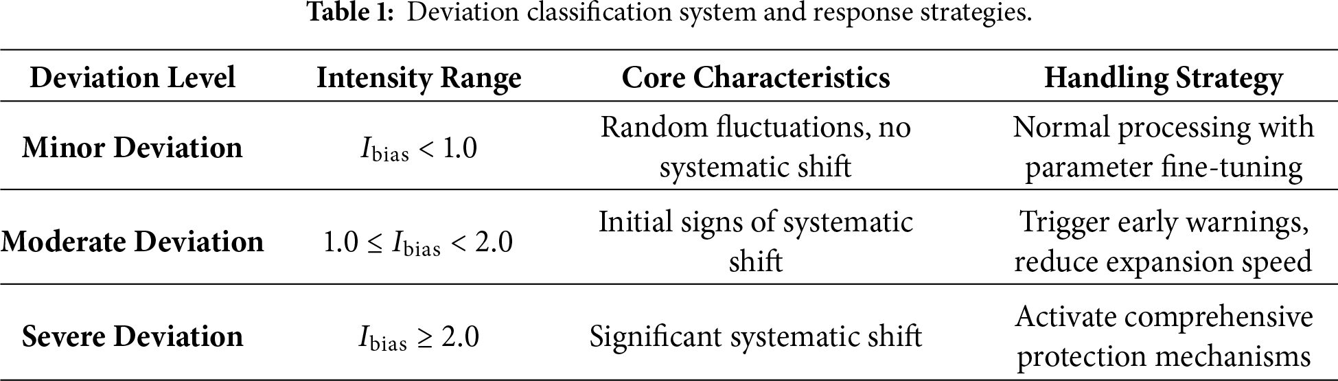
To quantify deviation severity, we introduce a long-term deviation intensity parameter that synthesizes magnitude and duration, mathematically characterizing systematic shift severity. Based on this metric, we define a three-tier deviation classification system:

•   Minor deviations: Maintain standard processing workflows.

•   Moderate deviations: Trigger early warnings, enhancing sensitivity by reducing window expansion rates and adjusting dynamic thresholds.

•   Severe deviations: Activate comprehensive protections, including fixed minimum window sizes and hybrid query routing.

The dynamic error threshold εdynamic is computed based on the residual sequence collected within the t-th sliding window Wt, whose window length is w and update step is Δw. The residual sequence in Wt is denoted as et={et,1,et,2,…,et,w}. By sorting et in ascending order, the corresponding order statistics are obtained as et,(1)≤et,(2)≤⋯≤et,(w).

The median of the residuals in the current window, denoted as Medt, is defined as

Medt={et,(w+12),ifwis odd,et,(w2)+et,(w2+1)2,ifwis even.(21)

The historical residual median mean, denoted as Medhist,t, is defined as the arithmetic average of the residual medians from the latest three historical sliding windows:

Medhist,t=13∑k=13Medt−k.(22)

The median absolute deviation (MAD) of the residuals in the current window is defined as

MADcurrent,t=median1≤i≤w(|et,i−Medt|).(23)

Based on the above definitions, the dynamic error threshold is computed as

εdynamic,t=Medhist,t+ωt⋅1.4826⋅MADcurrent,t.

Here, the constant 1.4826 is a scale factor that converts the median absolute deviation to the standard deviation under the Gaussian distribution assumption. The adaptive weight ωt is introduced to adjust the sensitivity of the threshold to different deviation levels, where ωt=0.8 corresponds to slight deviations and ωt=0.6 corresponds to severe deviations.

The calculation of the long-term bias intensity Ibias integrates data distribution shift and residual features, and its formula is as follows:

Ibias=|μcurrent−μhistory|σcurrent+0.4×Medtεdynamic.(24)

Among them, the historical window mean μhistory is the average of the means of the two most recent historical windows, and the mean of a historical window is calculated as:

μhistory=μk−1+μk−22.(25)

where μk−1 and μk−2 are the averages of timestamps in the (k−1)-th and (k−2)-th historical windows, respectively. The calculation formula is:

μk−1=1wk−1∑i=1wk−1xi.(26)

The current window mean is:

μcurrent=1w∑i=1wxi(27)

and the formula for the current window standard deviation is:

σcurrent=1w∑i=1w(xi−μcurrent)2(28)

Med denotes the median of residuals in the current window, εdynamic is the dynamic error threshold, and 0.4 is the weight coefficient that balances “mean drift” and “residual bias”.

The following table further illustrates the intensity ranges, core characteristics, and handling strategies corresponding to different deviation levels, providing a concrete explanation of the quantitative assessment and response mechanisms within the three-tier deviation classification system. Further details are provided in Table 1.

3.5 Proof of Convergent Behavior

To ensure the stability and reliability of the SW-LI method in a dynamic blockchain data environment, this section analyzes its convergence from a theoretical perspective. Consider a dataset A consisting of N ordered data points {(ti,hi)}i=1N, where ti is strictly increasing, and an error threshold ε>0. The SW-LI construction algorithm is guaranteed to terminate in a finite number of steps and to output a piecewise-linear index such that the prediction error of each data point satisfies

|h^i−hi|≤ε.(29)

We prove this claim by construction. Define the following symbols:

•   Wmin=2 (minimum window size allowed by the algorithm).

•   Let Sk represent the current window at the time of k iteration.

•   Let pk represent the starting data point index of Sk.

The window shrink operation has a lower bound:

When there are data points in the window Sk that make the fitting error greater than ε, the algorithm executes Wk1←⌈Wk/2⌉. Since Wmin=2, and for any two data points (ti,hi),(tj,hj)(i<j), there is a unique linear function f such that f(ti)=hi and f(tj)=hj, where the fit residual is zero. Therefore, when the window size shrinks to 2, the error condition must be met and the shrinkage process is terminated.

The window expansion and movement process is limited: When the window Sk meets the error condition, the algorithm executes:

•   Record the linear parameters of the window.

•   Update window size: Wk1←Wk+Δw.

•   Move window start: pk1←pk+Wk.

Since the total number of data points N is limited, and the starting point moves forward by at least Wmin=2 points after each window is accepted, the entire data can be traversed through a maximum of ⌈N/2⌉ windows.

4  Data Query

4.1 Data Query Procedure

When a node receives a query request for a specific timestamp ts, such as a request related to a transaction, the processing procedure is as follows:

(1) Locate the segment:

Quickly locate the corresponding segment using the learned index to identify the timestamp ts and the corresponding segment interval.

(2) Obtain model parameters:

Retrieve the linear model parameters (slope ak and intercept bk) for the identified segment.

(3) Compute predicted value:

Using the obtained linear model parameters, calculate the predicted block height corresponding to timestamp as: h^s=akts+bk. Since the predicted value may not be an integer, rounding (up or down) is required to determine the nearest actual block height stored in the system. To address potential discrepancies between the predicted block height and the true mapping from timestamp to block height, an error tolerance ε is introduced. The actual block height hs corresponding to the queried transaction will therefore lie within an interval around the predicted value, that: [h^s]−ε≤hs≤[h^s]+ε.

(4) Locate the actual block:

The query starts from the block corresponding to the predicted position and then searches the neighboring blocks. Because the sliding-window mechanism significantly improves the accuracy of learned index construction, the query begins at the block indicated by the predicted value. If the target transaction is not found in this block, the search is expanded to the immediate blocks on the left and right of the predicted position, scanned sequentially, and then continues to traverse blocks outward on both sides until the target transaction is identified. As shown in Algorithm 2.

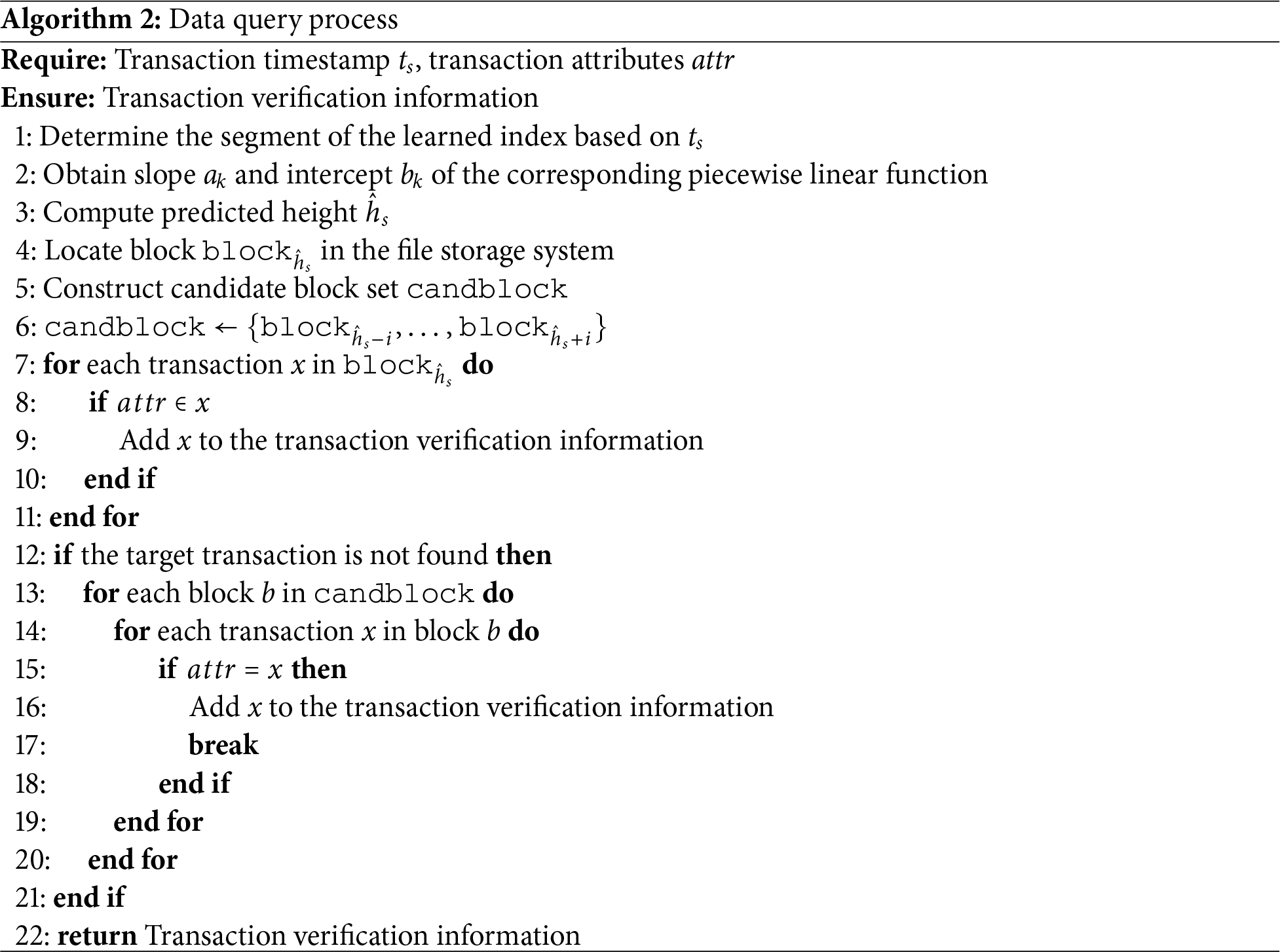
If you need to inquire about transactions that include a certain attribute within a specific time range, The process is similar to a single transaction inquiry. First, According to the time interval [t1,t2]. Obtain the corresponding piecewise function from the learning index, and based on this, calculate the corresponding block height h^1 and h^2. Then, Traverse each block of the interval [h^1−ε,h^2+ε] one by one. Retrieve transaction information that contains specific attributes, and add this transaction information to the verification information.

Within the block. Transaction data is organized in the form of a Merkle tree. When the node is defined to the target transaction within the block. Return the transaction information and part of the information in the Merkle tree as verification information to the client. The client performs the corresponding hash calculation on the received verification information. Obtain the root hash value of the Merkle tree, and compare it with the root hash value in the synchronized block header information. If both are consistent. This proves the existence of the message and its correctness.

4.2 Query Complexity Analysis

Considering that timestamps have an order property. This study uses a balanced binary tree structure to store the parameters of the piecewise linear function. In this way, the time complexity of querying the piecewise linear function corresponding to a specific timestamp is O(log(n)). Among them, n is the number of segments. When predicting the block height of the exchanges to be queried. The complexity of finding the parameters of a piecewise linear function is O(log(n)). Among them, n is the number of segments. Inquiry about specific transaction information. It is necessary to carry out operations such as traversing the blocks within the error value range. When the prediction error bound n1 and the number of transactions per block n2 are treated as fixed constants, the maximum number of transactions that need to be examined during local search is bounded by n1 ∗ n2. Under this assumption, the local search incurs constant-time complexity, i.e., O(1). Therefore, in this case, the overall complexity of data querying is mainly determined by the complexity of searching for the parameters of the piecewise linear function, that O(log(n)).

5  Simulation and Experimental Analysis

5.1 Simulation

5.1.1 Experimental Platform

•   Processor: AMD Ryzen 5 3550H @ 2.10 GHz;

•   Memory: 16 GB RAM;

•   Software environment: Python 3.12.

5.1.2 Data Processing

We download blockchain data from the Ethereum mainnet, covering block heights in the range [0,80,000,000] and timestamps spanning [1, 455, 404, 053, 1, 455, 876, 350]. The raw Ethereum dataset [19] is partitioned into consecutive block segments, and the number of transactions within each block is further reorganized to construct datasets of different scales, parameterized by the combination of block count and transactions per block.

For the evaluation dataset, timestamps and block heights are reorganized into (ti,hi) pairs for index construction. Using a set of random seeds [1,30], we perform stratified random sampling on the test dataset. For each seed, 1000 timestamps are sampled, and for each timestamp, one transaction is randomly selected from the corresponding block. This process yields 30 independent query workloads for evaluating timestamp-to-transaction queries.

5.1.3 Simulation Process

Our dataset consists of approximately 25,000 blocks, each containing 400 to 2000 transactions. For evaluation, we conducted 30 experimental trials. In each trial, a set of 1000 transactions was randomly sampled from the dataset. For the same transaction set, we executed both the proposed algorithm and the compared algorithm.

5.1.4 Key Metrics

(1)   Index construction time: The time required to build the learned index over a dataset containing N block data points;

(2)   Index size: The storage space occupied by the learning index structure;

(3)   Accuracy: The prediction error between learned index values and actual values;

(4)   Query time: The time required for timestamp-to-transaction queries.

The query latency Tql primarily consists of the prediction time Tpre and the transaction traversal time Ttxn:

Tql=Tpre+Ttxn(30)

The prediction time Tpre is the time required to predict the block height from an input timestamp. The traversal time Ttxn is the time spent searching within the predicted block for the corresponding transaction information. The number of transactions that need to be traversed equals the prediction error multiplied by the number of transactions per block.

We compare the proposed method with Anole [20], SWS-OGD [21], and B+ tree indexing to comprehensively evaluate its effectiveness in terms of construction cost, storage overhead, and query performance.

5.2 Parameter Sensitivity and Efficiency Analysis of SW-LI

To better understand how key parameters influence the efficiency, scalability, and robustness of SW-LI, we conduct a series of targeted experiments. Specifically, we evaluate how different parameter configurations affect query latency, index construction cost, and index compression behavior across varying data scales, with the goal of identifying robust default settings and characterizing key design trade-offs.

As shown in Fig. 2, a grid-based evaluation of the weighted distance parameter α (with β=1−α) and the threshold coefficient γ shows that the average query latency is minimized near α≈0.5. Deviating from this setting—either toward smaller or larger α—leads to a marked increase in latency, indicating that overly skewed weight assignments incur additional query overhead. Moreover, γ exhibits a well-defined optimal range: when α≈0.5, γ≈1 yields the lowest latency, whereas values of γ that are either smaller or larger result in noticeable performance degradation. Overall, the system remains robust for α∈[0.35,0.65]; however, combining extreme α values with suboptimal γ settings substantially deteriorates query efficiency. These findings support adopting symmetric weighting (α=β=0.5) and setting γ close to 1 to achieve consistently low and stable query latency across parameter configurations.

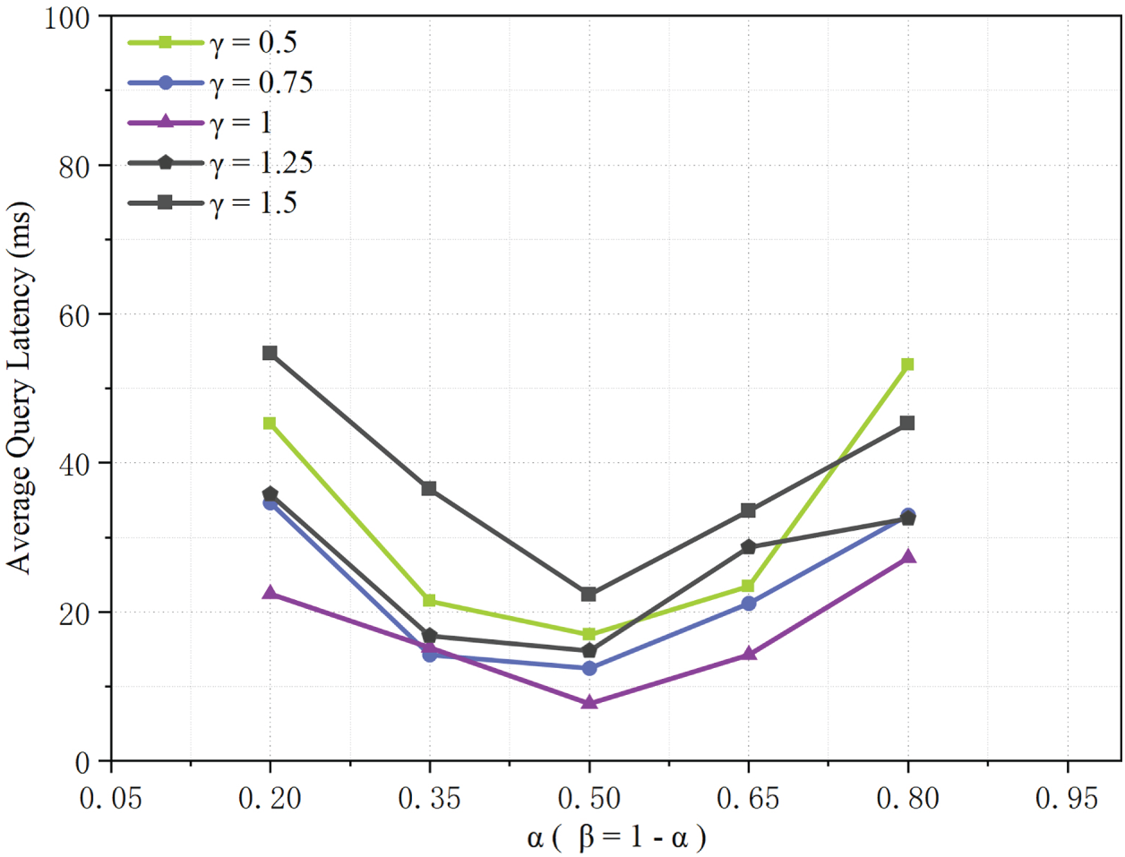
Figure 2: Impact of α,β,γ on average query latency.

As shown in Fig. 3, the index construction time increases nearly linearly with the number of blocks for window sizes W∈2,5,10,20,30,40. The choice of the initial window size has only a marginal effect on overall construction efficiency: at a fixed scale, construction times across different W values are tightly clustered, and even at the largest scale (25,000 blocks) the maximum gap remains on the order of milliseconds. Although larger W introduces a modest additional construction overhead, it does not change the overall scaling trend. This suggests that the initial window size primarily affects the computational granularity during the cold-start phase, while leaving the system’s overall efficiency and scalability largely unchanged. Overall, these results indicate that the system is robust to the choice of W and corroborate the default parameter setting.

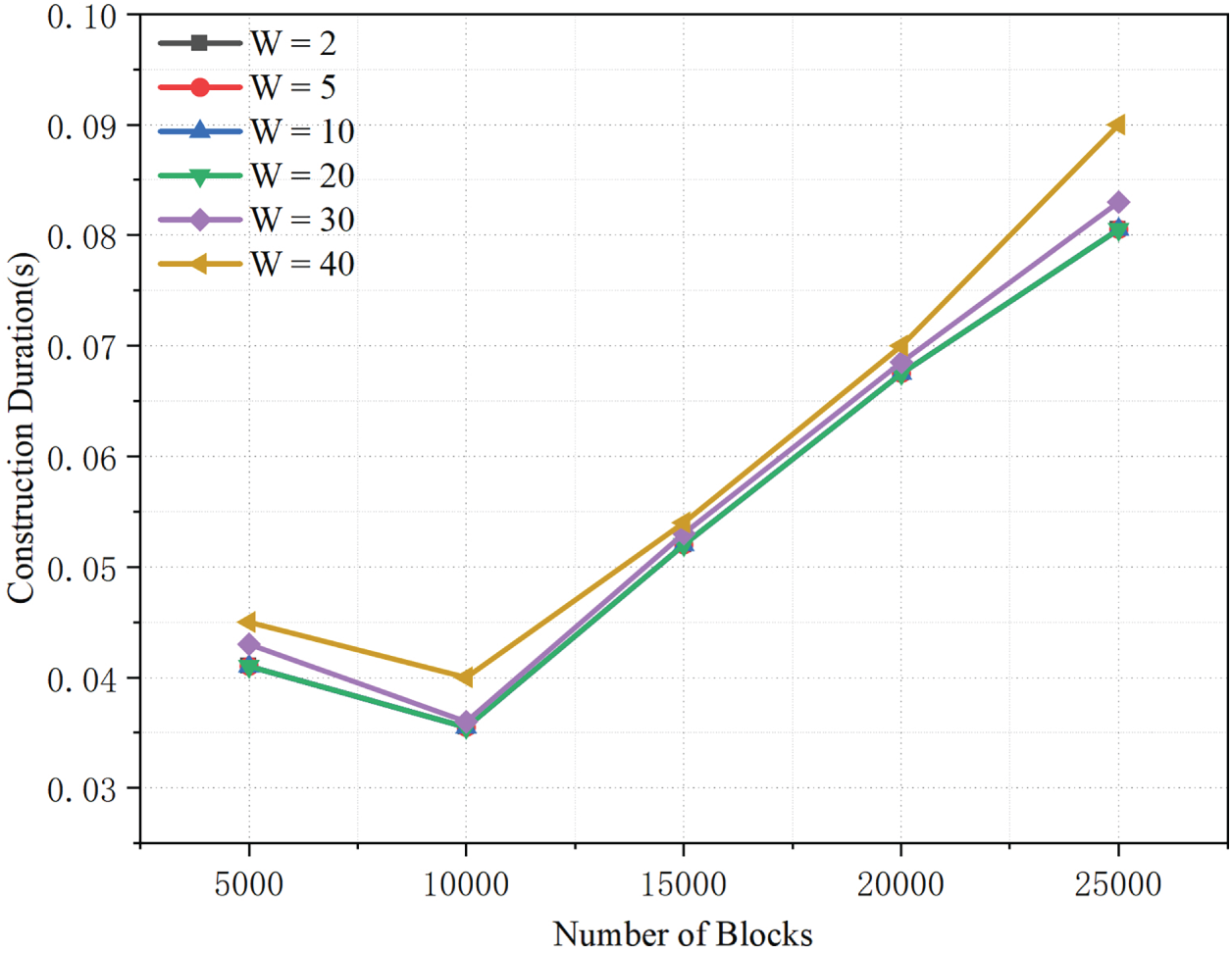
Figure 3: Index construction time under varying block counts and initial window sizes W.

As shown in Fig. 4, a larger window expansion step slightly reduces the index size. This suggests that less frequent updates improve index compactness. For a fixed step size, a smaller error bound requires more segments to meet the accuracy constraint, which increases the index size. With a dynamic error threshold, the bound can tighten in some windows. This often produces more segments and a slightly larger index than fixed-threshold settings. Overall, the results show a trade-off between update granularity (step size) and error control in index overhead.

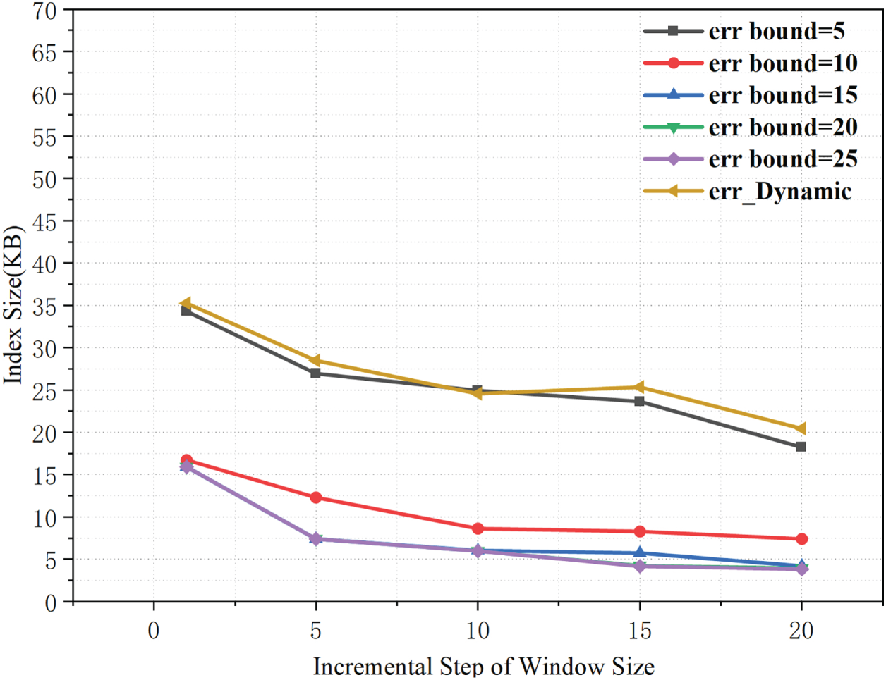
Figure 4: Effects of step size and error threshold on index size.

As shown in the Fig. 5, the overall index construction time decreases as the window expansion step increases. A larger step size allows the sliding window to reach an appropriate scale more quickly, thereby reducing the number of window expansions and model updates and lowering the construction overhead. For a fixed step size, a smaller ε imposes a stricter accuracy constraint. This typically requires more segments and more frequent fitting and updates, leading to longer construction time. The εdynamic setting also tends to incur higher construction time, because the threshold may tighten in certain windows, increasing segmentation and triggering more adjustments. Overall, these results indicate that construction efficiency is jointly determined by the step size and the strength of error control, highlighting the trade-off between construction cost and accuracy constraints.

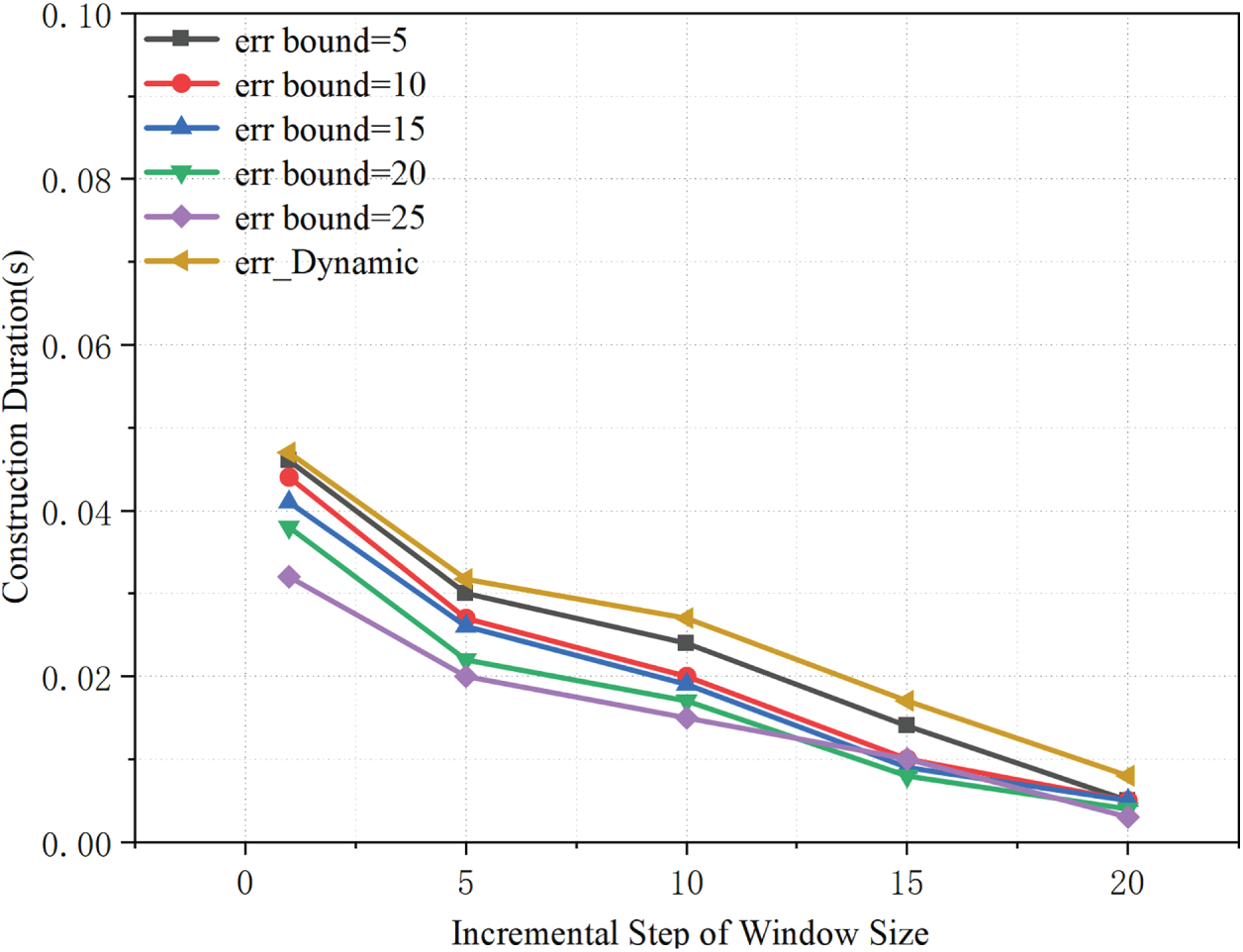
Figure 5: Effects of step size and error threshold on construction time.

As shown in Fig. 6, the average error increases slightly as the window expansion step grows, indicating that overly large step sizes reduce the granularity of window adjustment and thus incur a modest loss in accuracy. For a fixed step size, a larger fixed error bound ε permits a coarser approximation with fewer segments, leading to higher average error. In contrast, the εdynamic scheme adaptively adjusts error control according to data characteristics, achieving consistently lower and more stable errors and thereby providing better accuracy preservation.

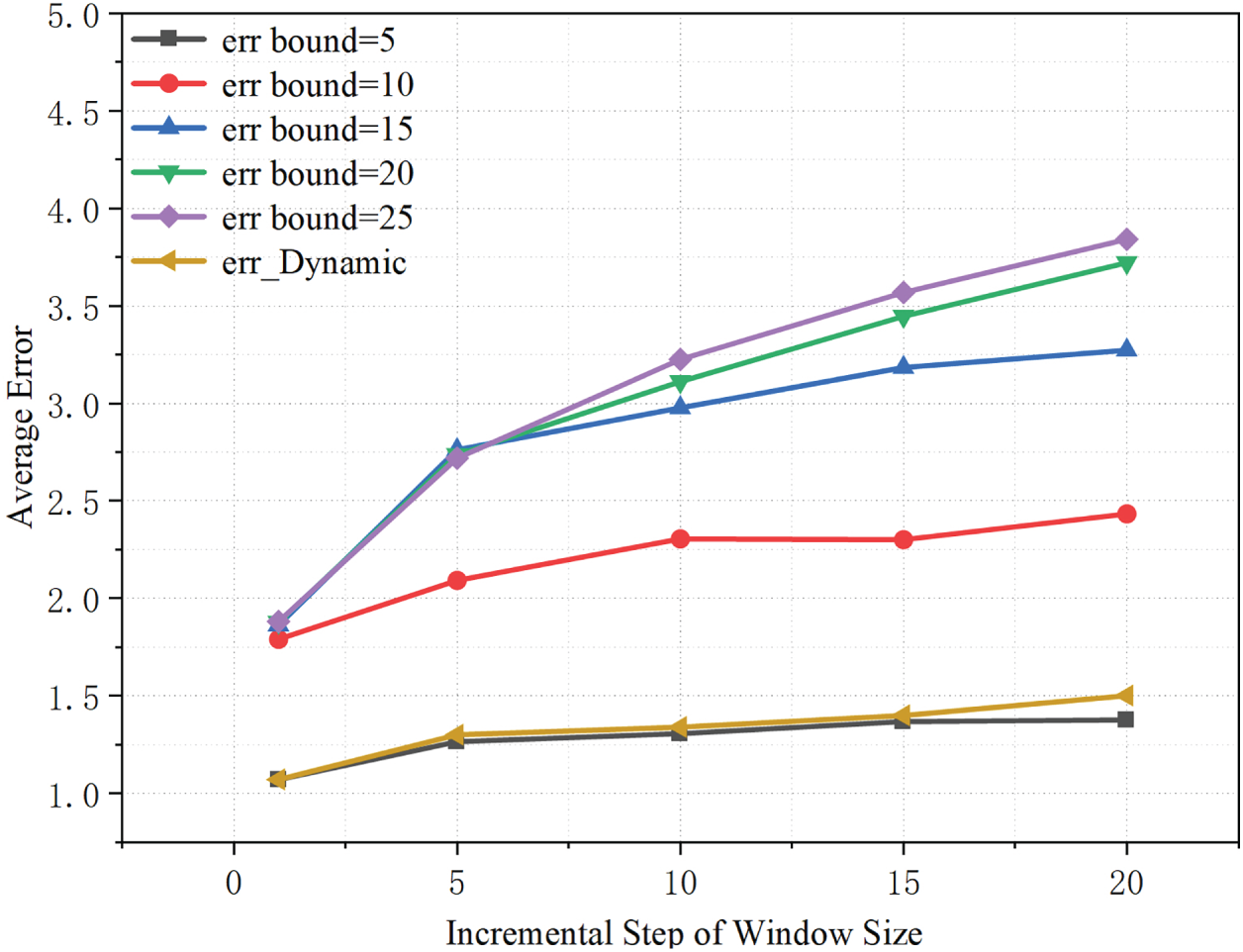
Figure 6: Effects of step size and error threshold on average error rate.

As shown in Fig. 7, the window expansion step has a limited impact on average query latency, with only minor fluctuations observed across different step sizes, suggesting that query-time overhead is not primarily governed by the window update granularity. For a fixed step size, a larger fixed error bound (ε) leads to higher latency because increased prediction error enlarges the search range and requires scanning more candidate transactions. In contrast, the εdynamic scheme consistently yields lower and more stable latency, indicating that adaptive error control effectively confines the scan range and improves query efficiency.

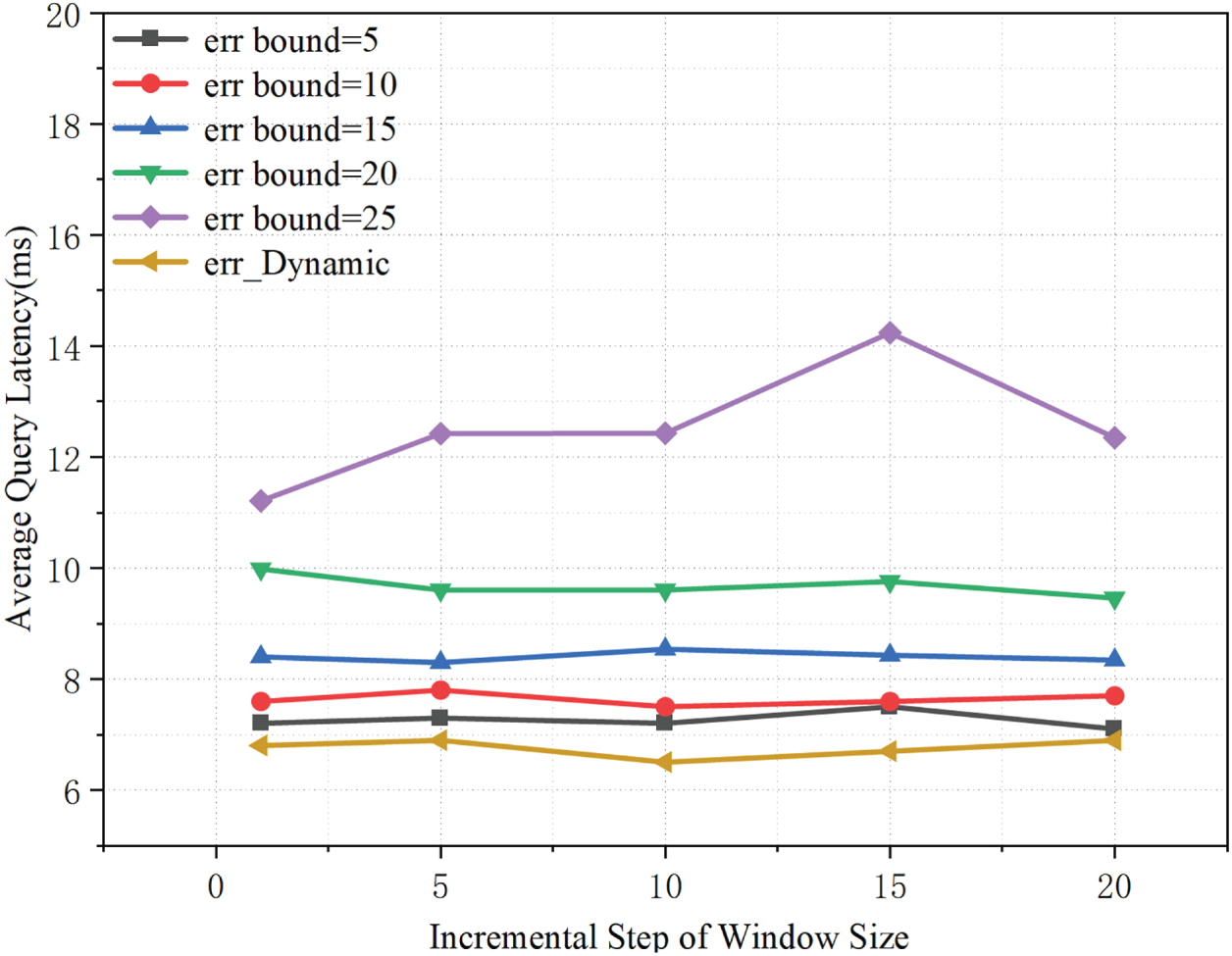
Figure 7: Effects of step size and error threshold on average query latency.

5.3 Ablation Study of SW-LI Components

In order to quantify the contributions of DupCheck, dynamic thresholds, and deviation protection to the algorithm, we conducted tests and comparisons using the SW-LI core as the baseline. As shown in Fig. 8, DupCheck markedly reduces index size relative to the baseline SW-LI across all block scales by removing redundant data and reducing the number of indexed entries. By contrast, adopting a dynamic error threshold yields a slightly larger index, because segments are adjusted more frequently to satisfy adaptive error constraints. Despite this increase, the index size remains close to the baseline, indicating that the additional segmentation overhead is well controlled. Overall, DupCheck effectively lowers storage cost, whereas the dynamic threshold introduces a modest and acceptable size overhead in exchange for improved adaptability.

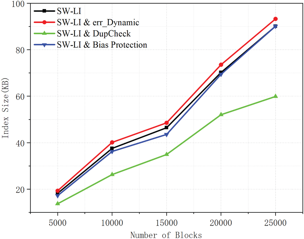
Figure 8: Index size comparison of SW-LI with dynamic error threshold, deduplication, and bias protection.

As illustrated in Fig. 9, DupCheck consistently reduces index construction time across all block scales by removing redundant data and thus lowering the effective indexing workload. By contrast, the dynamic-threshold variant incurs a slightly higher construction cost than the baseline, because adapting the error threshold increases the number of fitting operations during index building. Despite this overhead, the additional cost remains modest and the construction time still increases smoothly with the number of blocks, indicating that the cost of dynamic error control is well bounded.

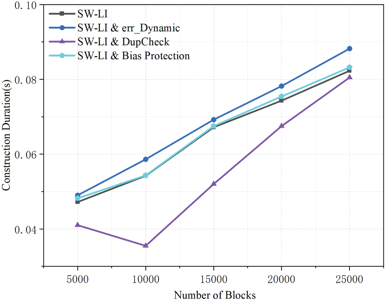
Figure 9: Comparison of index construction time for SW-LI and its variants with dynamic error threshold, deduplication, and bias protection.

As shown in Fig. 10, the dynamic threshold variant consistently achieves low average error across all block scales. This benefit stems from adaptive thresholding, which improves local fitting and mitigates systematic bias accumulation, thereby reducing average prediction error. By contrast, the baseline and DupCheck-enhanced variants yield higher average errors because they rely on static error-control mechanisms.

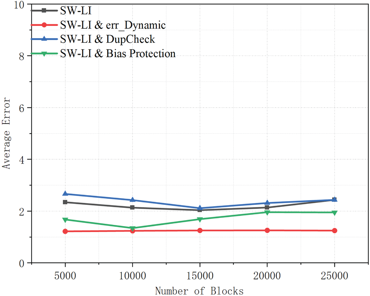
Figure 10: Average error comparison of SW-LI and its enhanced variants across different block scales.

As shown in Fig. 11, the maximum error results further confirm the benefit of bias protection. The bias-protected configuration yields the lowest and most stable maximum error among all variants, suggesting that its correction mechanism suppresses error amplification over time. By compensating for long-term bias, it prevents worst-case errors from escalating as the block scale grows. Overall, these results indicate that dynamic error control mainly improves average fitting accuracy, whereas bias protection is essential for bounding worst-case error. Together, they enhance the robustness of SW-LI under large-scale and dynamic workloads.

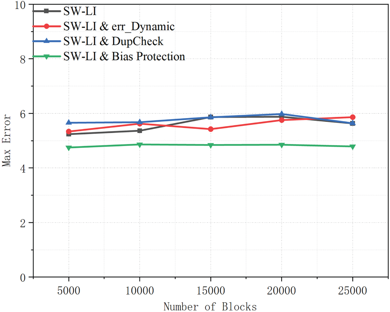
Figure 11: Maximum error comparison of SW-LI and its enhanced variants across different block scales.

As illustrated in Fig. 12, both DupCheck and bias protection consistently reduce query latency relative to the baseline SW-LI across different numbers of transactions per block. DupCheck achieves this improvement by removing redundant records, which reduces the indexed data volume and lowers the cost of prediction and lookup during query processing. Bias protection further decreases latency by mitigating accumulated prediction bias, thereby reducing the number of extra transactions accessed to meet the target query accuracy. In addition, the dynamic error threshold also outperforms the baseline: by maintaining smaller prediction errors, it limits unnecessary query expansions. Overall, these results suggest that both redundancy elimination and error control are key to improving query efficiency, enabling the enhanced variants to achieve lower and more scalable latency than the core SW-LI.

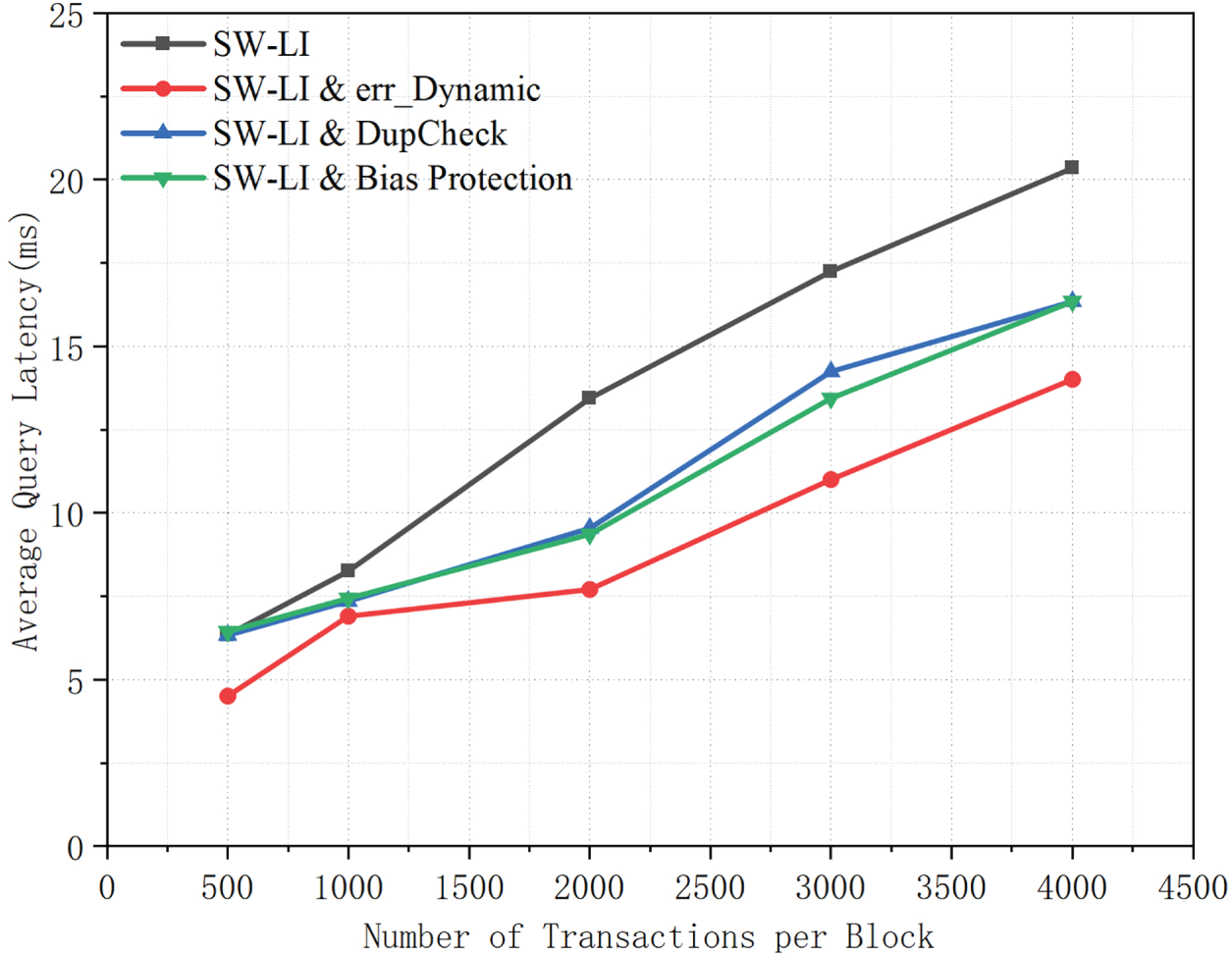
Figure 12: Average query latency of SW-LI and its enhanced variants under different numbers of transactions per block.

5.4 Learning Index Construction Efficiency

This experiment evaluates the performance of four methods (SW-LI, Anole, SWS-OGD, B+ tree) in terms of index construction time and index size under varying block quantities. The experimental parameters are configured as follows: both the Anole method and our proposed SW-LI method adopt an error threshold of 5. For the SW-LI method, the initial sliding window size is set to 2 with a window increment step of 5. Subsequent experiments will conduct sensitivity analysis on these two parameters (error threshold and window size) to investigate their specific impacts on learning index construction.

As shown in Fig. 13, the index construction time increases with the number of blocks for all four methods. SWS-OGD updates model parameters online, and therefore achieves the shortest construction time and the smallest storage overhead. In contrast, both Anole and SW-LI adopt piecewise linear regression, which requires additional fitting time and storage for segment parameters to enable fast query processing. The B+ tree baseline does not involve model fitting; it reorganizes the dataset into a tree structure and thus exhibits relatively shorter construction time. Overall, the variance exhibits only minor fluctuations, indicating that the performance is stable across all settings.

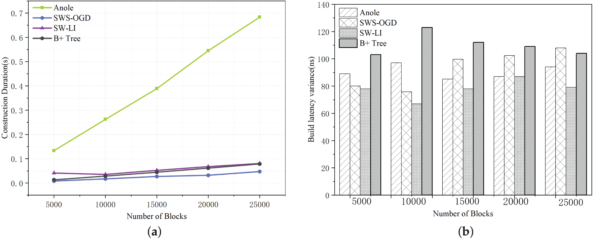
Figure 13: Comparison of index construction results under different numbers of blocks (W=2, Δw=5, ε=5, Transactions = 500): (a) Index construction time; (b) Build latency variance.

Compared with the Anole method, SW-LI significantly accelerates index construction by selecting data intervals using a sliding window and fitting multiple data points through matrix operations. However, since the window size in SW-LI is dynamically adjusted based on an error threshold, the number of generated segments is typically higher than that of Anole’s point-wise fitting strategy—particularly when a lower error threshold is applied. Consequently, the storage requirement of SW-LI tends to be relatively larger, as illustrated in Fig. 14. Although the index size can be reduced by merging adjacent segments with similar parameters, this optimization introduces additional computational overhead.

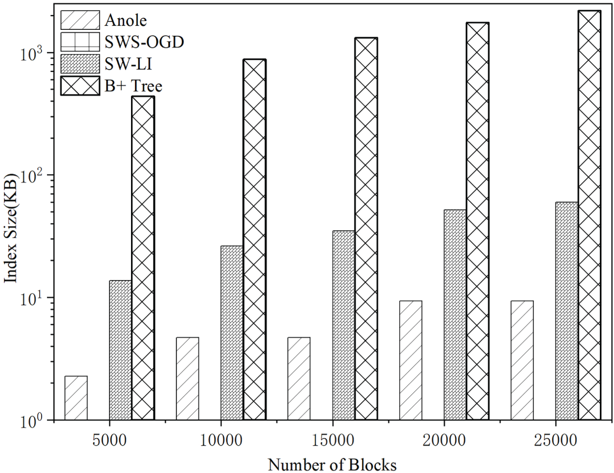
Figure 14: Learning index size across different block counts (W=2, Δw=5, ε=5, Transactions = 500).

Despite the comparatively higher storage demand of the SW-LI method, its absolute storage overhead remains efficient. As shown in Fig. 14, even when the number of blocks reaches 25,000, the size of the learned index constructed by SW-LI is only around 60 KB. This demonstrates that SW-LI provides a significant advantage in construction speed (compared to Anole), while maintaining high storage efficiency, making it well-suited for practical deployment scenarios. The B+ tree index is not a learned index, and its index data are not compressed, which results in substantially higher storage overhead.

5.5 Query Efficiency of Learning Indexes

During the data query process, nodes utilize the learned index (the B+ tree index is not a learned index and does not introduce errors) to predict the block height corresponding to a target transaction timestamp. However, there typically exists a discrepancy between the predicted and actual values. The total query latency is influenced by two primary factors: (1) the time required to predict the block height, and (2) the retrieval overhead caused by prediction errors, which necessitate scanning blocks in the vicinity of the predicted height.

In this experiment, learned indexes were first constructed for varying numbers of blocks. Subsequently, 1000 timestamps were randomly selected to evaluate block height prediction performance. The query effectiveness of the three methods (Anole, SW-LI, and SWS-OGD) was assessed using four metrics: average prediction error, maximum prediction error, prediction latency, and average query time. Furthermore, under a fixed block count of 20,000, the number of transactions per block was set to 500, 1000, 2000, 3000, and 4000, respectively. For each configuration, 1000 transactions were randomly selected for full queries (i.e., from timestamp to actual transaction data). The average query time was then computed to evaluate the end-to-end transaction query efficiency of each method.

As shown in Figs. 15 and 16, SW-LI achieves the highest precision, with both its average and maximum errors being significantly lower than the other two methods. SWS-OGD exhibits the largest errors due to its online parameter update mechanism for index construction. When data distribution undergoes significant variations, the prediction errors increase substantially. For instance, with 10,000 blocks, SWS-OGD demonstrates an average error of 25 and a maximum error reaching 75. Such substantial errors force nodes to scan numerous blocks and their internal transactions during retrieval, resulting in dramatically increased search overhead and consequently higher total query latency.

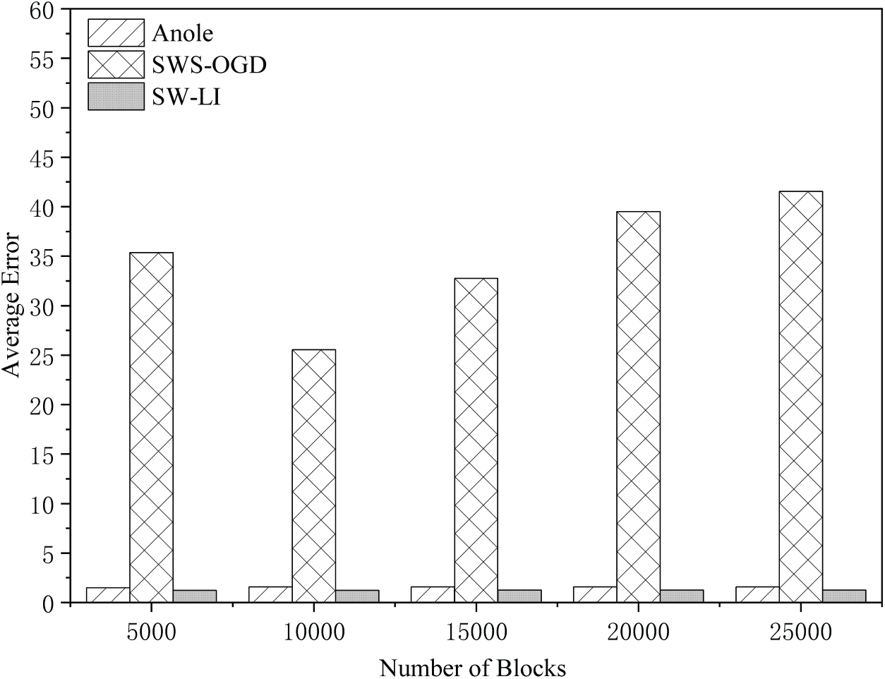
Figure 15: Average query error vs. block count (W=2, Δw=5, ε=5, Transactions = 500).

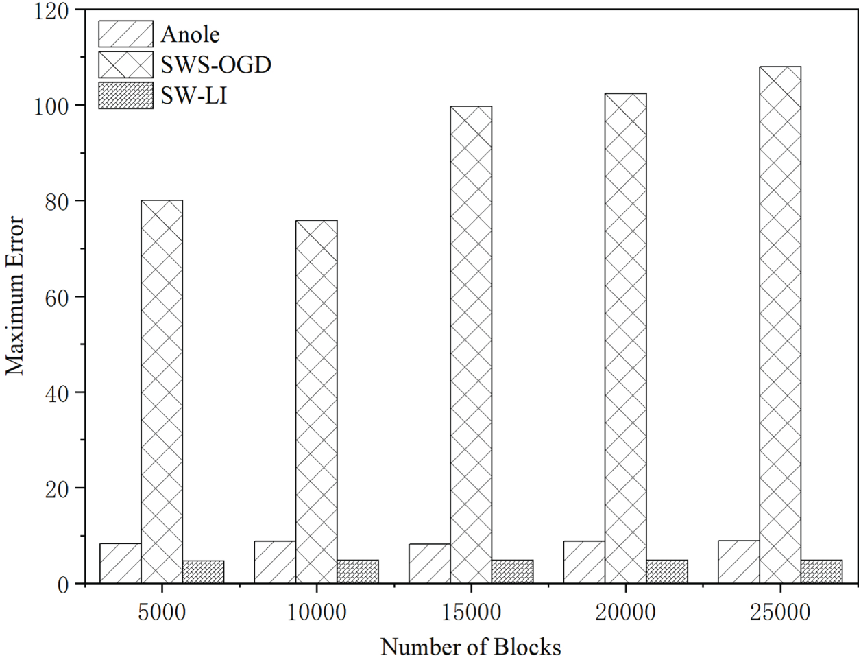
Figure 16: Maximum query error across varying blockchain sizes (W=2, Δw=5, ε=5, Transactions = 500).

Anole shows slightly higher average error than SW-LI, and its maximum error is approximately twice that of SW-LI. In our experiments, the error threshold is set to 5. Anole follows a point-by-point fitting strategy: once a new data point is tentatively assigned to the current segment, it refits the segment without re-checking whether all points still satisfy the error threshold. This “fit-after-inclusion” approach tends to bias the fitted curve toward data-dense regions when point distribution is non-uniform, leading to increased errors in sparse regions that may exceed the predefined threshold.

In contrast, SW-LI employs a rigorous verification mechanism: after performing global fitting for all points within a window, it individually checks each point’s prediction error to ensure strict compliance with the threshold. A segment is only finalized when all window points satisfy the error requirements. This approach strictly enforces global error constraints, effectively preventing the error amplification problem observed in Anole under non-uniform data distributions, thereby maintaining superior query accuracy.

As shown in Fig. 17, the prediction time of SW-LI is higher than that of Anole and SWS-OGD. This is because the SW-LI method segments the dataset based on sliding windows and fits the data within each segment. The increase in the number of blocks leads to a growth in the number of segments, thereby increasing the lookup time required to locate the target segment. The B+ tree lookup requires traversal of nodes on the tree, which is more time-consuming compared to the segment calculation performed by learned indexes. As shown in Fig. 18, the significance tests on the average error yield p<0.05 across all evaluated block scales, indicating statistically significant differences between SW-LI and the two baseline methods. Moreover, the comparison between SW-LI and Anole consistently produces smaller p-values, suggesting stronger statistical evidence of a difference under this pairing.

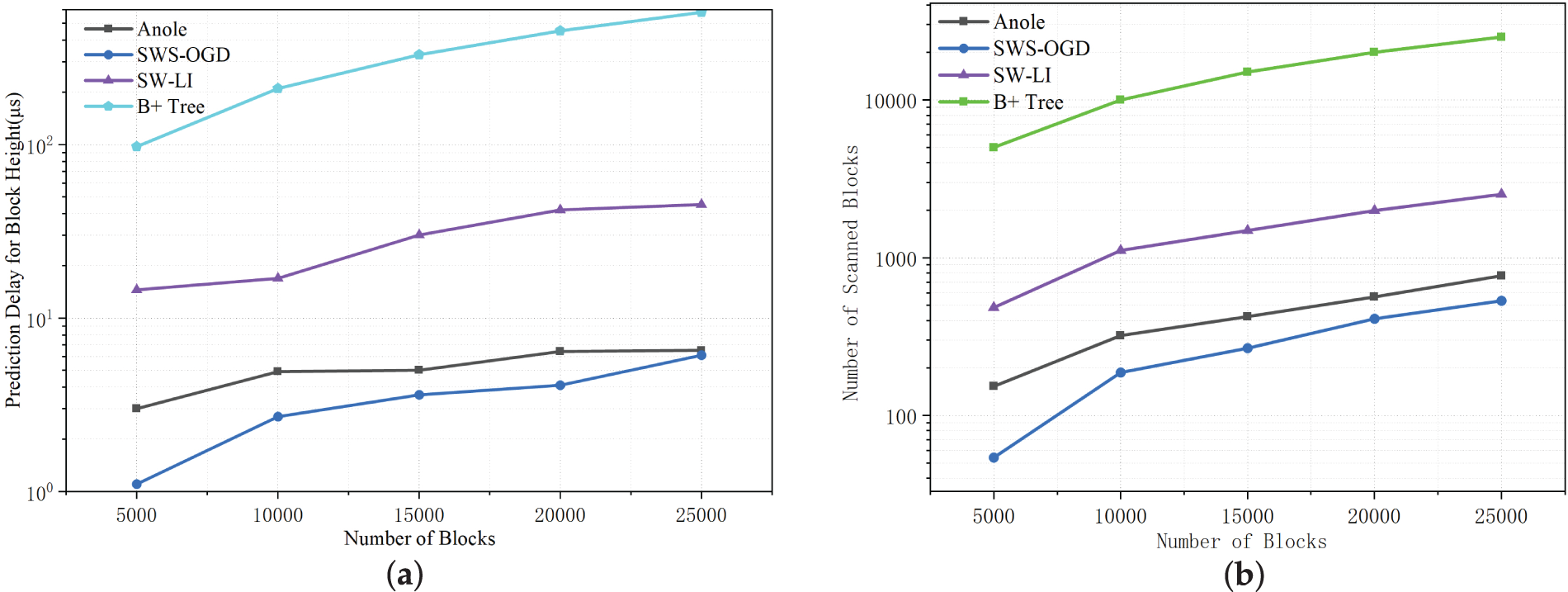
Figure 17: Comparison of block height prediction results under different numbers of blocks (W=2, Δw=5, ε=5, Transaction = 500): (a) Prediction delay for block height; (b) Number of scanned block.

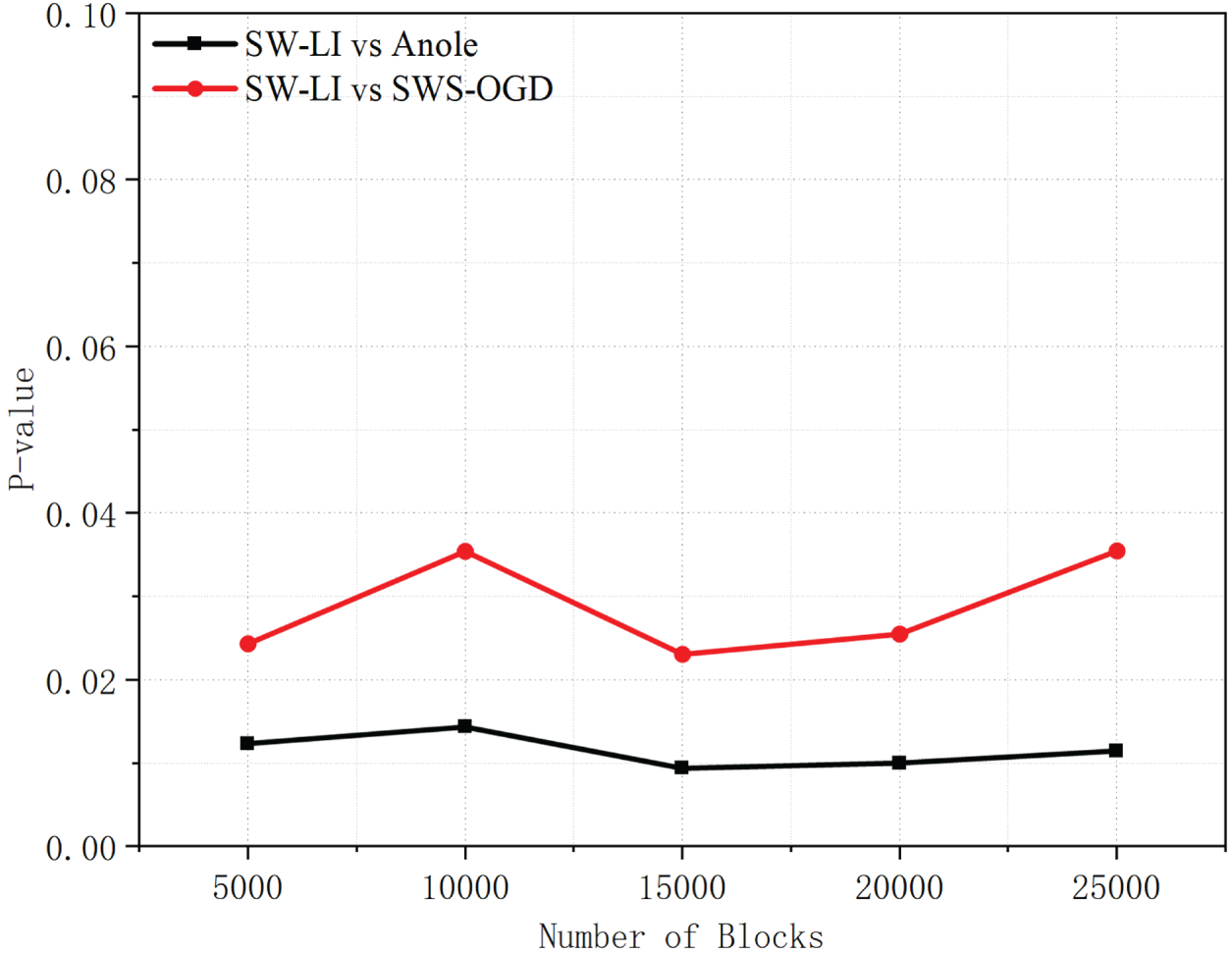
Figure 18: p-values of average error comparisons between SW-LI and baseline methods across different block scales.

As illustrated in Fig. 19, as the number of transactions per block increases, the advantage of the SW-LI method in total query latency expands significantly. The reason is that although SW-LI incurs slightly higher prediction overhead, its exceptionally low prediction error greatly reduces the number of blocks and transactions that need to be scanned. In contrast, the larger errors of Anole and SWS-OGD cause their block retrieval costs to surge with the growth in transaction volume. When a block contains 4000 transactions, the average total query latency of SW-LI is 46.15% lower than that of Anole and only 2.7% of SWS-OGD’s average query latency (i.e., approximately 37 times faster). B+ tree indexes maintain a relatively high index access time. This conclusively demonstrates SW-LI’s significant efficiency advantage in high-load, large-scale data query scenarios.

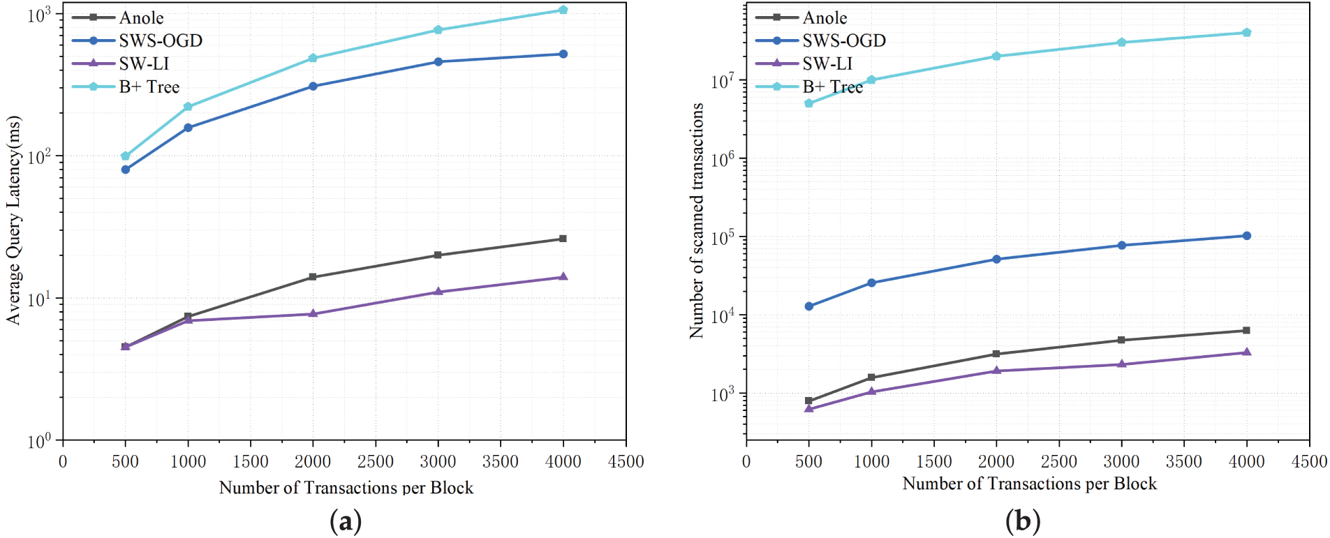
Figure 19: Comparison of transaction query results under different transaction quantities (W=2, Δw=5, ε=5, BlockNumber = 10,000): (a) Average transaction query latency; (b) Number of scanned transactions.

As shown in Fig. 20, the significance tests on query latency yield p<0.05 across all evaluated block scales, indicating statistically significant differences between SW-LI and the two baseline methods in terms of query time. Furthermore, the comparison between SW-LI and SWS-OGD consistently results in smaller p-values, suggesting stronger statistical evidence of a difference under this pairing.

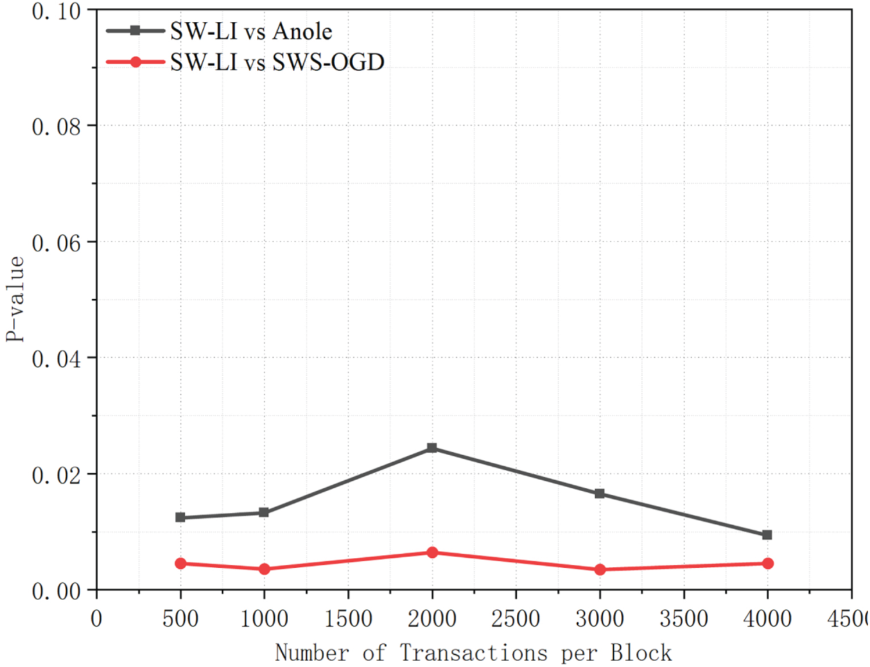
Figure 20: p-values of query latency comparisons between SW-LI and baseline methods under different numbers of transactions per block.

6  Conclusion

This paper proposes a sliding window-based learned index construction method for blockchain systems, termed SW-LI. The method employs a sliding window mechanism to select subsets of block data, efficiently establishing the mapping relationship between block timestamps and heights. It introduces a dynamic window resizing strategy: when the data distribution exhibits irregular patterns, the window automatically contracts to preserve fitting accuracy. Conversely, when the data follow regular patterns, the window expands to accelerate index construction. Experimental results demonstrate that with 5000 and 25,000 blocks, respectively, SW-LI reduces index construction time by 69.22% and 88.22% compared to Anole.

Regarding index size, SW-LI maintains a compact learned index of merely 60 KB for 25,000 blocks, with block height prediction completing in under 50 microseconds. The query performance shows remarkable advantages, when processing blocks containing 4000 transactions, SW-LI achieves 46.16% lower average query latency than Anole, and requires only 2.7% of SWS-OGD’s query latency (37× faster).

While the proposed method delivers superior performance in high-throughput blockchain systems, its effectiveness may be limited in low-throughput scenarios due to delayed index updates caused by slow block generation. Future work will focus on optimizing this mechanism to address index update challenges in low-throughput environments, thereby enhancing system performance across all operational scenarios.

Acknowledgement: We would like to thank Shenyang University of Technology, China for providing facilities and support for this study.

Funding Statement: This work was supported by the National Key Research and Development Program of China (No. 2022YFB3105100).

Author Contributions: Jun Qi: Conceptualization, Data curation, Writing—original draft, Methodology, Visualization, Validation. Chao Yang: Conceptualization, Visualization, Methodology, Writing—review and editing, Supervision. Junyou Yang: Resource, Data curation. Xinliu Wang, Haixin Wang, Huaqin Chen and Zhenyan Li: Writing—review and editing, Visualization, Methodology, Supervision. All authors reviewed and approved the final version of the manuscript.

Availability of Data and Materials: The data that support the findings of this study are available from the corresponding author, upon reasonable request.

Ethics Approval: Not applicable.

Conflicts of Interest: The authors declare no conflicts of interest.

Abbreviations

References

1. Zheng Z, Xie S, Dai H, Chen X, Wang H. An overview of blockchain technology: architecture, consensus, and future trends. In: Proceedings of the 2017 IEEE International Congress on Big Data (BigData Congress); 2017 Jun 25–30; Honolulu, HI, USA. p. 557–64. doi:10.1109/bigdatacongress.2017.85. [Google Scholar] [CrossRef]

2. Yang J, Dai J, Gooi HB, Nguyen HD, Wang P. Hierarchical blockchain design for distributed control and energy trading within microgrids. IEEE Trans Smart Grid. 2022;13(4):3133–44. doi:10.1109/tsg.2022.3153693. [Google Scholar] [CrossRef]

3. Lei L, Wang F, Zhao C, Xu L. Efficient blockchain-based data aggregation scheme with privacy-preserving on the smart grid. IEEE Trans Smart Grid. 2024;15(6):6112–25. doi:10.1109/tsg.2024.3435054. [Google Scholar] [CrossRef]

4. Dai J, Yang J, Wang Y, Xu Y. Blockchain-enabled cyber-resilience enhancement framework of microgrid distributed secondary control against false data injection attacks. IEEE Trans Smart Grid. 2024;15(2):2226–36. doi:10.1109/tsg.2023.3328383. [Google Scholar] [CrossRef]

5. Li B, Lin L, Zhang S, Xu J, Xiao J, Li B, et al. FlexIM: efficient and verifiable index management in blockchain. IEEE Trans Knowl Data Eng. 2025;37(6):3399–412. doi:10.1109/tkde.2025.3546997. [Google Scholar] [CrossRef]

6. Jia DY, Xin JC, Wang ZQ, Lei H, Wang GR. SE-chain: a scalable storage and efficient retrieval model for blockchain. J Comput Sci Technol. 2021;36(3):693–706. doi:10.1007/s11390-020-0158-2. [Google Scholar] [CrossRef]

7. Zhang H, Wei ZQ. Query model of blockchain system based on secondary index mechanism. J Comput Appl. 2022;42(S2):129–34. [Google Scholar]

8. Liu W, Wang D, She W, Song X, Tian Z. An efficient query method for blockchain traceability. J Appl Sci. 2022;40(4):623–38. [Google Scholar]

9. Wang JL, Zhang GY, Du LK, Li S, Chen T. A multi-level index construction method for master-slave blockchain. J Comput Res Dev. 2024;61(3):799–807. doi:10.7591/9781501738838-009. [Google Scholar] [CrossRef]

10. Yuan X, Huang LH, Chen ZK, Du XJ, Jiang H, Ma JF. Efficient and trusted query index model and method for blockchain data based on Merkle Patricia tree. J Chongqing Univ. 2023;46(7):9–22. doi:10.1109/iccc54389.2021.9674708. [Google Scholar] [CrossRef]

11. Wu H, Peng Z, Guo S, Yang Y, Xiao B. VQL: efficient and verifiable cloud query services for blockchain systems. IEEE Trans Parallel Distrib Syst. 2022;33(6):1393–406. doi:10.1109/tpds.2021.3113873. [Google Scholar] [CrossRef]

12. Muzammal M, Qu Q, Nasrulin B. Renovating blockchain with distributed databases: an open source system. Future Gener Comput Syst. 2019;90:105–17. doi:10.1016/j.future.2018.07.042. [Google Scholar] [CrossRef]

13. Xie Y, Wang Q, Li R, Zhang C, Wei L. Private transaction retrieval for lightweight Bitcoin clients. IEEE Trans Serv Comput. 2023;16(5):3590–603. doi:10.1109/tsc.2023.3290605. [Google Scholar] [CrossRef]

14. Jiang S, Cao J, Wu H, Chen K, Liu X. Privacy-preserving and efficient data sharing for blockchain-based intelligent transportation systems. Inf Sci. 2023;635:72–85. doi:10.1016/j.ins.2023.03.121. [Google Scholar] [CrossRef]

15. Ayub Khan A, Dhabi S, Yang J, Alhakami W, Bourouis S, Yee PL. B-LPoET: a middleware lightweight Proof-of-Elapsed Time (PoET) for efficient distributed transaction execution and security on Blockchain using multithreading technology. Comput Electr Eng. 2024;118:109343. doi:10.1016/j.compeleceng.2024.109343. [Google Scholar] [CrossRef]

16. Chang J, Lin LC, Li BH, Xiao J, Jin H. Efficient and verifiable query mechanism of DAG blockchain based on learned index. J Comput Res Dev. 2023;60(11):2455–68. [Google Scholar]

17. Kraska T, Beutel A, Chi EH, Dean J, Polyzotis N. The case for learned index structures. In: Proceedings of the 2018 International Conference on Management of Data; 2018 Jun 10–15; Houston, TX, USA. p. 489–504. doi:10.1145/3183713.3196909. [Google Scholar] [CrossRef]

18. Zhang Z, Jin PQ, Xie XK. Learned indexes: current situations and research prospects. J Softw. 2021;32(4):1129–50. [Google Scholar]

19. Zheng P, Zheng Z, Wu J, Dai HN. XBlock-ETH: extracting and exploring blockchain data from ethereum. IEEE Open J Comput Soc. 2020;1:95–106. doi:10.1109/ojcs.2020.2990458. [Google Scholar] [CrossRef]

20. Chang J, Li B, Xiao J, Lin L, Jin H. Anole: a lightweight and verifiable learned-based index for time range query on blockchain systems. In: Database systems for advanced applications. Cham, Switzerland: Springer Nature; 2023. p. 519–34. doi:10.1007/978-3-031-30637-2_34. [Google Scholar] [CrossRef]

21. Asiamah EA, Akrasi-Mensah NK, Odame P, Keelson E, Agbemenu AS, Tchao ET, et al. A storage-efficient learned indexing for blockchain systems using a sliding window search enhanced online gradient descent. J Supercomput. 2024;81(1):321. doi:10.1007/s11227-024-06805-3. [Google Scholar] [CrossRef]