A Multi-Source Fusion Spatiotemporal Neural Network Improved by Koopman Operators for Predicting Remaining Useful Life

1  Introduction

Prognostics and Health Management (PHM) is an interdisciplinary field integrating data science and engineering, playing a pivotal role in modern industry [1]. Due to its capability to effectively diagnose and predict the performance of complex equipment while ensuring system safety and reliability, it has garnered extensive research attention in recent years [2]. Remaining Useful Life (RUL) prediction is one of the core research areas in PHM, as it reveals the future degradation trends of equipment, enabling managers to formulate and implement targeted maintenance plans in advance. This ensures sustained and stable operation while reducing maintenance costs [3]. RUL prediction is critical in PHM, as reliable RUL estimation can minimize the risk of catastrophic failures [4].

Currently, the technical methods for RUL prediction are mainly divided into two categories: data-driven approaches and physics-based approaches. Physics-based approaches use the physical models of equipment and its main components for RUL prediction, which requires researchers to have an in-depth understanding of the system’s physical mechanisms [5]. However, with the rapid development of technology, the internal structure of modern equipment is highly complex and coupled, greatly increasing the difficulty of establishing accurate physical degradation models [6]. Moreover, physics-based methods are computationally intensive and cannot efficiently handle the continuous updating of nonlinear parameters. On the other hand, data-driven approaches do not need to consider the intrinsic physical behavior of the equipment. They can directly capture the relationship between equipment condition monitoring data and equipment degradation status, and thus achieve RUL prediction for the equipment [7]. Data-driven approaches are becoming increasingly popular in RUL prediction [8].

The two important branches of data-driven approaches are the deep learning (DL) and the machine learning (ML). The ML approaches mainly include Bayesian methods [9], particle filtering methods [10], and extreme learning machines [11]. However, the ML requires manual extraction of relevant data features, and if the feature extraction is not appropriate, it is difficult to achieve good predictive accuracy. The predictive performance of the ML is overly dependent on the quality of data features and often overlooks the temporal dependencies in the data. In contrast, the DL approaches excel at feature extraction and processing. The DL approaches eliminate the need for manual feature extraction, directly learning complex feature representations from the data [12]. From data input to RUL output, the DL follows an end-to-end training process, effectively mitigating human factors [13]. Compared to the ML, the DL offers superior robustness and predictive accuracy.

At present, mechanical systems are rapidly evolving towards automation and intelligence, with increasing complexity. Their operations and loads are unstable, leading to a strong nonlinear trend in the degradation trajectory of system performance, making the fault patterns of the system more difficult to grasp [14]. The temporal and spatial characteristics of system monitoring data are the two most fundamental dimensions [15]. Capturing the spatial characteristics of the data becomes particularly important. However, most existing RUL prediction methods focus on modeling the temporal characteristics of time series, neglecting the spatial relationships between data variables, and the modeling of the unstable changes in equipment performance degradation is not yet sufficient. Simultaneously, the level of model prediction and the measurement capability of state information has not yet attracted widespread attention in terms of the uncertainty of RUL prediction, leading to a decrease in the credibility of predictions [16]. Most existing studies do not provide interval probability prediction methods for RUL, and there is an insufficient quantification of RUL uncertainty.

In response to the aforementioned issues, the main contributions of this work are:

(1) A moving average-based temporal decomposition block (TDB) is introduced, and then the RUL prediction model that combines the Koopman operator with gated recurrent units (GRU) networks is proposed, using the Koopman operator for linearization of nonlinear features, enhancing the model’s dynamic prediction performance on complex time series data.

(2) We propose a STAr (STar Aggregate Redistribute) module dedicated to the extraction of spatial dependencies inherent in sequential data. By performing feature aggregation followed by a redistribution operation, the module bolsters the model’s interpretability of cross-variable interactions within multivariate temporal inputs.

(3) An integrated framework that couples ensemble learning with KDE is established to derive interval-type probabilistic RUL predictions, thus furnishing a systematic avenue for uncertainty quantification. Validation against four synthetic turbofan engine deterioration datasets reveals that our model consistently surpasses alternative approaches in both point and interval prediction performance.

The subsequent sections are arranged as follows. Section 2 details the core methodology of this work, encompassing three major modules: TDB, Koopman-GRU, and the channel interaction learning block. With respect to RUL uncertainty measurement, we devise an ensemble scheme coupled with KDE to provide probabilistic characterizations. Section 3 presents empirical evaluations performed on the C-MAPSS dataset to substantiate the efficacy of our model. Section 4 wraps up the main findings and identifies several worthwhile topics for subsequent exploration.

With the advancement of data mining capabilities and sensor technology, data-driven RUL prediction methods are increasingly gaining attention [17]. ML-based and DL-based RUL prediction methods represent the two primary data-driven approaches for RUL estimation. While their comparative analysis has been presented in the Introduction, this section further elaborates on DL-based RUL prediction methodologies [18]. CNNs struggle to capture the dependencies in time series and require high-quality and normalized data. Furthermore, CNNs adjust the parameters of the convolutional kernels and fully connected layers through backpropagation algorithms, which require a substantial amount of parameter tuning [19]. Fu et al. constructed a novel multi-channel attention dual-task TCN, integrating first prediction time detection with RUL prediction, enhancing the sensitivity to early failure detection [20]. Compared to CNN, TCN can capture long-term dependencies more effectively and is more stable and efficient in training than RNN. However, TCN has limited modeling capacity, may require more memory during testing and evaluation, and its application is still mainly limited to a single scale, lacking a sufficiently large receptive field. Chang et al. used heterogeneous Bi-GRU for RUL prediction, combining positive and negative time series with Bi-GRU to derive the degradation trend of equipment performance [21]. LSTM and its variants solve the problem of CNN’s difficulty in capturing temporal dependencies and can also eliminate the gradient explosion phenomenon of RNN to a certain extent [22]. Compared to TCN, they require less data storage during testing and evaluation. However, these methods are not strong in capturing multivariate spatiotemporal features from multi-sensor data. Due to the large number of training parameters, the training time for LSTM is relatively long, which can easily lead to the overfitting of training variables [23].

The above research has mainly focused on modeling the temporal characteristics of time series, neglecting the spatial relationships between different sensors. Combining Graph Convolutional Networks (GCN) with various sequential models to form Spatio-Temporal Graph Neural Networks (STGNN) is another popular approach in the field of spatio-temporal sequence prediction, such as the integration of GCN with RNN [24]. However, STGNN face computational inefficiency issues. Therefore, it is still worth further exploration on how to effectively model both the temporal and spatial patterns of data simultaneously. Moreover, most studies have not provided a probability prediction method for RUL intervals, resulting in insufficient quantification of uncertainty in RUL prediction.

From this, it can be concluded that the research work that can effectively predict the unstable changes in equipment performance degradation trends, enhance the comprehensive modeling ability of multivariate time series by capturing spatial features, and quantify the uncertainty of RUL prediction is still a challenging problem. Specifically, the main problems existing in current research, which are also the focus of this paper, are:

(1) The operations and loads during equipment operation are usually unstable, hence its degradation trajectory is unstable and highly nonlinear, posing a challenge to RUL prediction. Most existing studies struggle to effectively model the unstable changes in equipment degradation trends.

(2) Most existing RUL prediction methods concentrate on modeling the temporal characteristics of time series, neglecting the spatial relationships between different sensors, thus there is a need to enhance the comprehensive modeling capability of multivariate time series.

(3) Most existing studies do not provide interval probability prediction methods for RUL, and there is insufficient quantification of the uncertainty in RUL predictions.

2  Methodology

2.1 Overall Architecture

This paper proposes a Koopman operator-based spatiotemporal neural network integrated with multivariate fusion for RUL prediction, aiming to fully capture the multi-source features during the equipment degradation process for accurate forecasting, named the MST-K model. The model framework is shown in Fig. 1. To better describe the complex dynamic processes in system degradation, a Koopman-GRU module is introduced, which uses GRU to extract temporal dependency features and employs the Koopman operator for linear modeling of these features in a high-dimensional space. A CILB then captures the inter-sensor dependency using a series core representation between channels, enhancing the feature expression capability. Finally, a prediction module generates the final RUL forecast using a residual structure’s linear layer, ensuring the model maintains good predictive performance when dealing with complex dynamics and multi-channel dependent data.

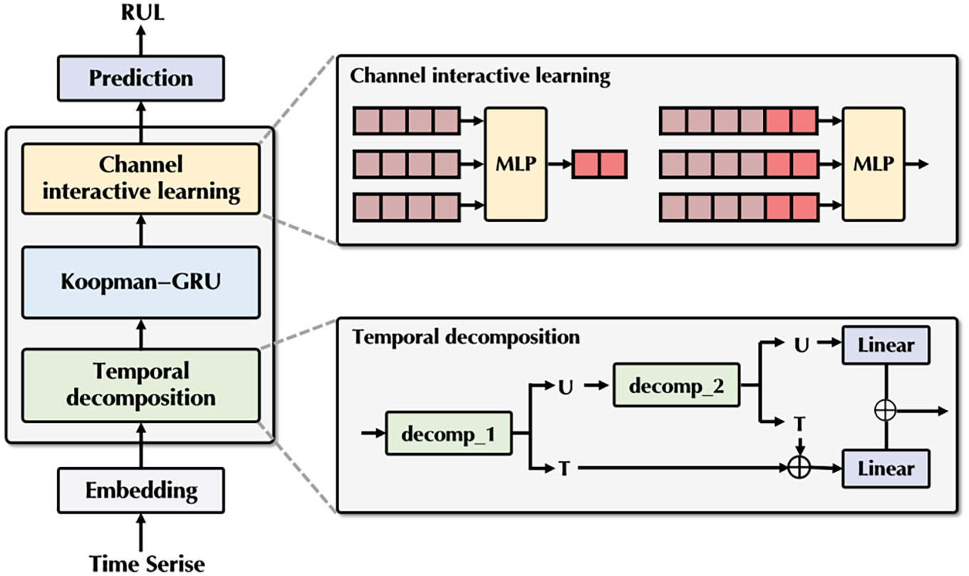
Figure 1: Overall architecture of the model.

2.2 Model Input

To obtain a learnable data representation, a standard 1 × 1 convolution is employed to preliminarily fuse inter-channel features, thereby mapping the input data into a high-dimensional latent space, as shown in Eq. (1).

O=Embedding(X)(1)

In Eq. (1), O represents the preprocessed multi-sensor time-series data, while Embedding(∙) denotes the operation of preliminary inter-channel feature fusion using standard 1 × 1 convolution.

2.3 TDB

Affected by unstable loads and varying operating conditions, the degradation trajectory of equipment often exhibits nonlinearity. Therefore, it is crucial to accurately identify the stable degradation trends and unstable variations in time series data. The former reflects the long-term degradation behavior of the equipment state, while the latter captures short-term fluctuations and anomalies. This paper employs a moving average-based TDB [25], to better separate trends and unstable components, thereby providing a more sufficient feature representation for subsequent models. To more effectively separate the two, a quadratic decomposition method is employed, as follows:

Ot_1=avgpool(padding(X))(2)

Ou1=O−Ot_1(3)

Ot_2=avgpool(padding(Ou1))(4)

Ou2=Ou1−Ot_2(5)

where avgpool(∙) denotes the average pooling operation, padding(∙) represents the zero-padding operation at the boundaries in average pooling, Ot_1 corresponds to the trend component obtained from the first decomposition, Ou1 signifies the unstable component derived from the first decomposition, Ot_2 indicates the trend component of the second decomposition, and Ou2 stands for the unstable component of the second decomposition. Compared to the single-pass version, the two-pass filter achieves a flatter passband (better trend preservation) and a steeper stopband attenuation, which effectively removes residual oscillations while preserving the underlying degradation trajectory. From a signal processing perspective, additional passes would further suppress noise, but at the cost of significantly amplified phase lag. For RUL prediction, temporal fidelity is as critical as noise suppression—excessive smoothing delays the detection of degradation onset, leading to overestimated RUL. Thus, two passes represent the optimal trade-off between denoising adequacy and phase lag minimization. In recent years, linear layers have been proven effective in modeling the inherent complex patterns within time series [26]. Through linear transformation of the trend and unstable components, dimensional alignment and information enhancement in the feature space are achieved. The trend components from the two-level decomposition are summed element-wise to form an integrated trend representation, which comprehensively captures multi-scale trend characteristics during equipment degradation.

P=Linear1(Ou2)+Linear2(Ot_1+Ot_2)(6)

In Eq. (6), Linear1 denotes the linear transformation operation for the unstable component, Linear2 represents the linear transformation operation for the trend component, and P stands for the integrated trend representation.

2.4 Koopman-GRU

For the task of RUL prediction, handling the complex dynamic processes in sequences is a critical challenge in model design. Koopman operator theory provides strong support for addressing this issue by mapping nonlinear dynamic systems to a high-dimensional linear space to capture linear trends within the system. This paper designs a Koopman-GRU module, which first extracts local dependency features from the time series through GRU, and then uses the Koopman operator to model the linear dynamic evolution of these features in the high-dimensional space, to better describe the complex dynamic characteristics during the system’s degradation process. Our Koopman-GRU module consists of four sequential steps that together embed the Koopman evolution into the GRU’s hidden state transition. Step 1: GRU Candidate Hidden State; Step 2: Observable (Lifting Functions) Construction; Step 3: Koopman Linear Evolution; Step 4: Hidden State Update via Projection. The Koopman operator is not used as a standalone predictor or feature extractor; rather, it is embedded within the GRU’s hidden state transition. The GRU first computes a nonlinear candidate hidden state ht−. This candidate is lifted to the Koopman observable space gt;=[xt;ϕ(xt);ht−]. The trainable Koopman matrix K advances this observable linearly: gt+1pred=Kgt+gt. Finally, a linear projection extracts the hidden-state component: ht=Wproj+gt+1pred. This ht; replaces the raw GRU output and is passed to the next time step. In this way, the Koopman operator serves as a stability regularizer that linearly constrains the GRU’s nonlinear dynamics, preventing long-term error accumulation. The complete loss function used to train the Koopman operator includes a linearity loss, a consistency loss between the Koopman-predicted and GRU hidden states, and a multi-step prediction loss. The spectral properties of K are enforced via eigenvalue reparameterization to ensure stable long-term evolution.

rt=σ(ptWxr+ht−1Whr+br)(7)

ut=σ(ptWxu+ht−1Whu+bu)(8)

ct=RELU(ptWxc+rt⊙Whc+bc)(9)

ht=(1−ut)⊙ht−1+ut⊙ct(10)

where ⊙ denotes element-wise multiplication, σ represents the sigmoid activation function, pt signifies the input at time step t, and Wxr, Whr, Wxu, Whu, Wxc, Whc, br, bu, and bc are all model parameters. The GRU structure can effectively capture local dependencies within a time series and obtain the hidden representations H={h1,h2,…,ht,…,hT} for all time steps.

ht=(1−ut)⊙ht−1+ut⊙ctH^=Wproj⋅H(11)

where H^ represents the feature representation in the high-dimensional space, and Wproj denotes a linear layer with a Relu activation function. Subsequently, the Koopman operator performs a linear transformation on the feature H^, capturing the dynamic evolution within the sequence, and re-maps it to the same feature dimension as the original data. In standard deep Koopman architectures, the training objective typically consists of three complementary loss components. The total loss is a weighted combination: L=Lrecλ1+Llinλ2+Lpredλ3. This paradigm ensures that the learned Koopman matrix K truly captures the linear evolution of the observables. Lrec ensures the encoder-decoder mapping is invertible; Llin enforces linear dynamics in the lifted space; Lpred ensures accurate future state prediction.

H^′=K⋅H^(12)

Z=Winv⋅H^′(13)

where K is a trainable Koopman matrix that represents the linear dynamic relationship within the feature space. Specifically, instead of directly optimizing the raw matrix K, we parameterize it as: K=VΛV−1. Λ is a diagonal matrix of eigenvalues, V is a matrix of eigenvectors (trainable). Winv denotes a linear layer with a Relu activation function.

2.5 CILB

In multivariate time series forecasting, capturing the dependencies between various channels is an important means to improve prediction accuracy. In previous studies, the attention mechanism has been widely used. However, traditional attention mechanisms incur computational complexity proportional to the square of the number of channels. Therefore, the STar proposed by Han et al. was introduced [27]. This method aggregates information from each channel to generate a series core representation and redistributes this representation to each channel, enhancing the feature expression capability of each channel. The STar can reduce complexity and effectively model the dependencies between channels in multivariate data, as shown in Fig. 2.

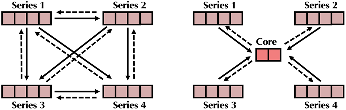
Figure 2: The schematic diagram of the STAR.

Core representations are extracted from the inputs of various channels and used to capture global information. For the aforementioned multivariate time series feature representation Z∈RT×C, each channel input is denoted as zi∈RT. Specifically, the sequence representation of each channel is first projected, and then a channel-level representation is generated through a multi-layer perceptron (MLP).

ui=MLP1(zi)(14)

In Eq. (14), MLP1(∙) denotes the MLP operation for the i-th channel, while ui represents the feature representation at each channel level, whose output dimension is defined as the series core.

Subsequently, a stochastic pooling mechanism is employed to integrate these channel-level representations, generating a series core representation. This core representation effectively extracts important information from all channels, capturing the global characteristics of the entire time series.

U=Sto_Poolomh(u1,u2,…,ui)(15)

In Eq. (15), Sto_Poolomh(∙) denotes the stochastic pooling operation, while U represents the global core representation. Max pooling selects only the maximum activation, discarding all other information. This is suitable for classification tasks where the most salient feature matters, but for RUL prediction, degradation information is distributed across multiple sensors/channels—a sensor that is not maximally activated at the current time step may still carry critical trend information. Average pooling preserves all features but treats them equally, which dilutes the contribution of informative channels. Stochastic pooling strikes a balance: it samples channels according to a probability distribution proportional to their activation values, thereby preserving diversity while still giving higher selection probability to more informative channels.

After generating the series core representation U, it is necessary to redistribute it to each channel to enhance the local feature representation of each channel. Therefore, the global core representation U is concatenated with the feature representation ui of each channel to produce an enhanced channel representation fi.

fi=Concat(ui,U)(16)

In Eq. (16), Concat(∙) denotes the concatenation operation.

At present, the features of each channel contain both the local information of that channel and the global information from other channels. Finally, another multi-layer perceptron is used to project the concatenated features, generating the final channel feature representation z~i.

z~i=MLP2(fi)(17)

2.6 Prediction Block

Recent studies have indicated that simple linear models, which are capable of handling non-linear dependencies, also offer fast inference speeds. Therefore, a residual-structured linear layer has been designed to serve as the final output module. A linear layer is used to obtain the ultimate prediction result Y, as shown in Fig. 3.

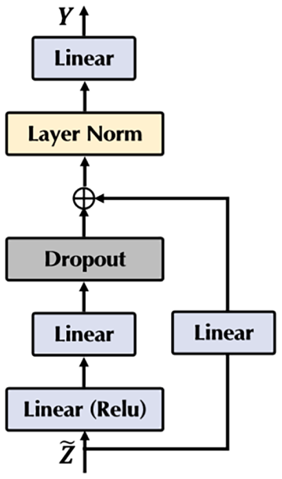
Figure 3: The structure of the prediction block.

2.7 Ensemble Learning

There are four main steps involved:

(1) Sensor data is preprocessed, involving selecting appropriate sensors, standardizing the data, applying smoothing techniques, organizing the training and testing samples as required by the model, and assigning RUL labels to the training samples.

(2) The MST-K network architecture is constructed and the network is trained with the training set data, with the best model being saved.

(3) Utilizing test data, the well-trained MST-K model is employed for RUL prediction.

(4) The results, including point predictions and interval probability predictions, are outputted. Subsequently, an evaluation of the model’s performance is conducted.

Our ensemble uncertainty quantification framework generates 100 differentiated predictions per model through two complementary stochastic mechanisms. Mechanism 1: Monte Carlo Dropout (MC-Dropout); Mechanism 2: Stochastic Pooling. Following the Monte Carlo Dropout framework, we enable dropout during inference (i.e., at test time). For each of the 100 predictions, we perform a different random dropout mask applied to the GRU layers: (1) During training, dropout is used for regularization (dropout rate = 0.2); (2) During inference, we keep dropout active rather than turning it off; (3) Each forward pass uses a different random subset of neurons in the GRU layers. This produces a different prediction for the same input with each pass.

The STAR (Stochastic sTAtus-feature inteRaction) module uses stochastic pooling to capture channel interactions. During training, stochastic pooling samples channels according to a probability distribution proportional to their activation values. Crucially, we also use stochastic pooling during inference for uncertainty quantification: (1) For each of the 100 predictions, the STAR module performs independent random sampling from the channel probability distribution; (2) Different samples produce different channel selection patterns, leading to different predictions.

3  Experiments

3.1 Settings

(1)   Benchmark Datasets

The dataset information is shown in Table 1.

Fig. 4 illustrates the main components of a turbofan engine, such as the fan, combustor, and high-pressure compressor (HPC) [28]. Each dataset consists of three subsets: a training set, a testing set, and the actual RUL for each engine in the testing set. The training set data with complete degradation trajectories are used to train the proposed MST-K model, while the testing set data with incomplete degradation trajectories are used to simulate online applications for obtaining point predictions and interval probability predictions of RUL.

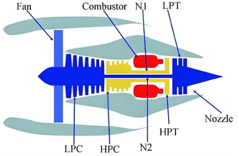
Figure 4: The structural diagram of the turbofan engine.

(2)   Data pre-processing

The dataset comprises 21 available sensor measurements. However, not all sensor data contains information that aids in RUL prediction. For instance, measurements from multiple sensors remain constant throughout the engine’s lifecycle, rendering such data meaningless for RUL forecasting [29].

Monoi=|dx(i)>0M−1−dx(i)<0M−1|(18)

Corri=|∑t=1M(xt(i)−x¯t(i))(t−t¯)||∑t=1M(xt(i)−x¯t(i))2∑t=1M(t−t¯)2|(19)

Crii=θ⋅Corri+(1−θ)⋅Monoi−γ(20)

From Table 1, it can be observed that the fault mode does not significantly impact the sensor monitoring data, it need not be considered during data preprocessing. However, varying operating conditions affect the values of sensor monitoring data, complicating the analysis and prediction of RUL. It is crucial to account for the influence of operating conditions during data preprocessing [30]. To simplify the processing of sequences and achieve better RUL prediction results, an exponential weighted moving average was applied to the full lifecycle data collected by the sensors [31].

Xj′=β∗Xj+(1−β)∗Xj−1′(21)

The lower the value of β, the better the smoothing effect. Although smoothing the sensor monitoring data will lose some of the original information, since the purpose of modeling is not to detect faults or anomalies, but to obtain the overall degradation trend, therefore, smoothing treatment will not have an adverse effect on the data. Before constructing the MST-K model, due to the inconspicuous performance degradation, it is necessary to revise the RUL labels. As shown in Fig. 5, a piecewise linear function with an inflection point at 125 was adopted due to its good model generalization performance. Subsequently, the model was run on a personal computer equipped with an AMD R7-4800H (2.90 GHz) with Radeon Graphics and 16.0 GB of memory, operating on the Microsoft Windows 10 system.

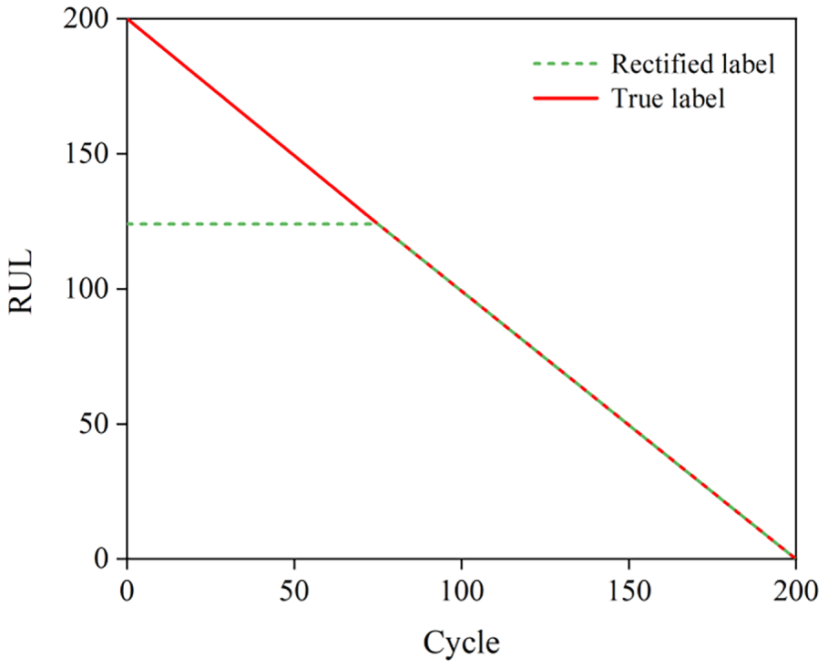
Figure 5: The revised engine RUL label.

(3)   Implementation details

The parameters involved in the MST-K model include feature dimension, training epochs, batch size, time step, and optimizer. Before training the network, the time step for prediction was set to 30. In the sensor selection process, considering that monotonicity and correlation are equally important, the value of θ in Eq. (17) was set to 0.5. The threshold γ was empirically set to 0.2, with sensors numbered 1, 5, 6, 10, 16, 18, and 19 being discarded. FD001/FD003 (single operating condition): The data is relatively homogeneous, allowing for smaller batch sizes (64–128) and moderate learning rates. FD002/FD004 (multiple operating conditions): The data is more heterogeneous, requiring larger batch sizes (256–512) to stabilize gradient estimates and lower learning rates to avoid overfitting to dominant conditions. FD003/FD004 (multiple fault modes): The presence of multiple degradation patterns necessitates different regularization strengths (dropout and weight decay). This variation is a well-known phenomenon in transfer learning and multi-domain RUL prediction.

The weight factor θ = 0.5 is selected to achieve an equal balance between two complementary criteria: (1) Correlation with RUL: Captures sensors whose absolute magnitude degrades monotonically with RUL (e.g., temperature and pressure sensors that rise steadily with degradation); (2) Monotonicity: Captures sensors whose trajectory shape is monotonic but may have a delayed or nonlinear relationship with RUL (e.g., sensors that exhibit accelerated degradation near the end of life).

The threshold γ = 0.2 is selected based on three considerations: (1) Statistical significance: With n = 128 of Batch size in FD001, a Pearson correlation coefficient of |r| ≥ 0.2 corresponds to a p-value < 0.005 (two-tailed test). This ensures that all retained sensors have statistically significant linear relationships with the RUL, minimizing the inclusion of noise-dominated or irrelevant sensors. (2) Empirical sensor analysis in C-MAPSS: In the C-MAPSS dataset, sensors with |r| < 0.2 typically exhibit either: Flat or highly noisy trajectories with little degradation information, or highly redundant information already captured by other sensors with stronger signals.

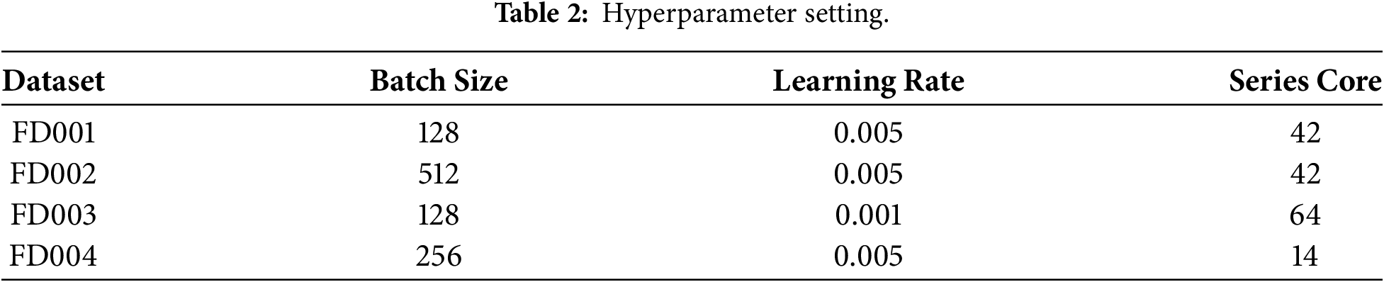
The hyperparameters reported in Table 2 were obtained through dataset-specific optimization (Bayesian optimization performed separately on each sub-dataset). The observed differences primarily reflect the following factors: (1) Data heterogeneity: FD002 and FD004 (multiple operating conditions) require larger batch sizes and lower learning rates to stabilize gradient estimates across diverse data distributions. (2) Degradation complexity: FD003 and FD004 (multiple fault modes) benefit from different regularization strengths (dropout and weight decay) to prevent overfitting to specific fault patterns. The optimizer used was the Adam optimizer, with 100 training epochs and an early stopping mechanism implemented, the settings for batch size, learning rate, and series core parameters varied for each sub-dataset, Table 2 shows this situation.

(4)   Valuation metrics

The RMSE measures the deviation between actual and predicted values, given by following equation [32]:

RMSE=1n∑i=1n(r^i−ri)2(22)

Usually, compared to predictions that are greater than the actual failure time, there is a preference for predictions that are less than the actual failure time. This preference is primarily because when predictions are less than the actual failure time, maintenance personnel will typically take action earlier to prevent engine failure. Consequently, predictions greater than the actual failure time are penalized more severely than those less than the actual failure time. The S-score is represented as follows:

S−score=∑i=1nedia−1(23)

where n is the number of test samples and di = r^i−ri. When di < 0, a = −13; otherwise, a = 10. The RMSE value and the S-score value assess only the performance of point RUL predictions. The α-Coverage (Prediction Interval Coverage Probability, PICP) metric must be defined based on whether the predicted intervals contain the ground truth, not the reverse. The credibility diagram for probabilistic forecasts are used to assess the quality of the prediction intervals constructed by probabilistic predictions, that is, the degree of match between the predicted probabilities and observed outcomes [33].

α−Coverage=1n∑i=1nℐ(α)i(24)

ℐ(α)i={1,ri∈[ri^0.5−0.5α,ri^0.5+0.5α]0, Otherwise (25)

where α ∈ [0, 1] is a parameter defined, [ri^0.5−0.5α,ri^0.5+0.5α] is therefore the α-level confidence interval. The α-Mean width is average width of α-percent confidence interval estimated for the RUL distribution of test sample i [34].

α−Meanwidth=1n∑i=1n(ri^0.5−0.5α,ri^0.5+0.5α)(26)

3.2 Results

(1)   RUL point prediction

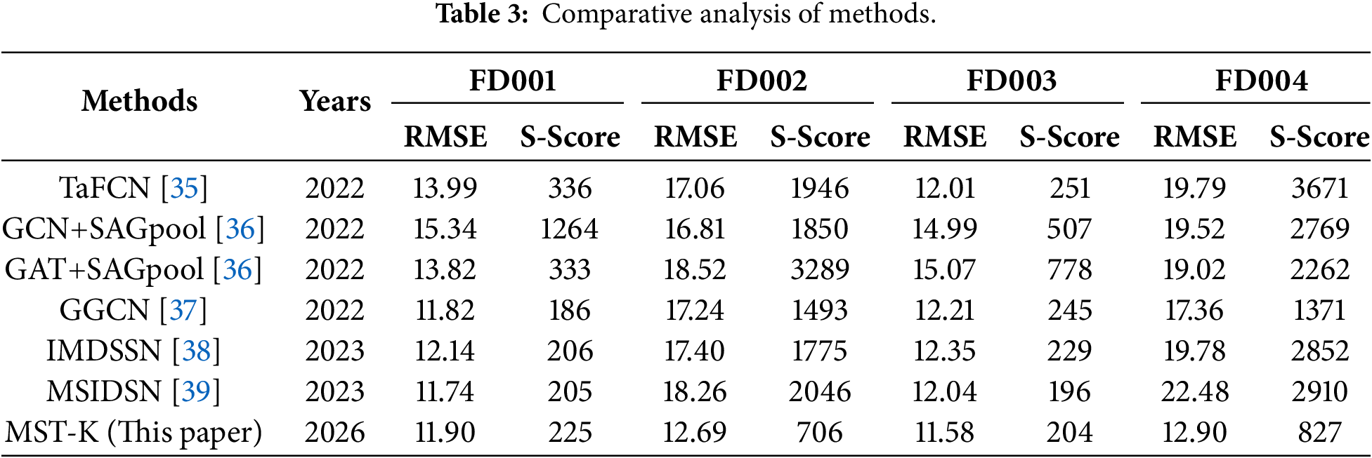
Fig. 6 illustrates the change in loss values for the MST-K model in both the training and validation sets. The model did not reach the maximum training epochs and stopped early at the 21st training epoch, at which point the best model was saved. Table 3 presents the RMSE and S-score values for RUL point predictions, with the best results highlighted in bold.

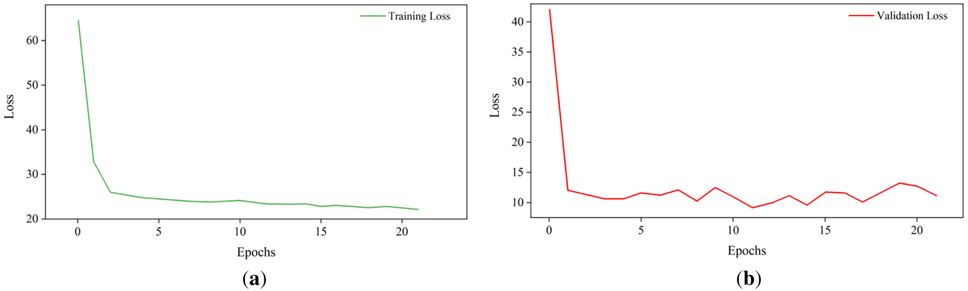
Figure 6: Changes in loss values of MST-K model: (a) training set; (b) validation set.

Further comparison of the RUL point predictions with actual value is made. When making Fig. 7, the actual value lengths corresponding to all test samples are first sorted in ascending order along the horizontal axis and matched with the RUL point predictions for each test sample. As the engine cycle count increases, the RUL predicted by the MST-K model gets closer to actual value. This indicates that the accuracy of MST-K model’s RUL point predictions generally increases over time, mainly because more and more engine status data are detected as time progresses, allowing the MST-K model to predict the engine’s RUL more accurately. As shown in Table 1, the FD001 sub-dataset provided 100 training samples, and the data was collected under a single operating condition; whereas the FD004 sub-dataset was collected under six different operating conditions but only provided 249 training samples.

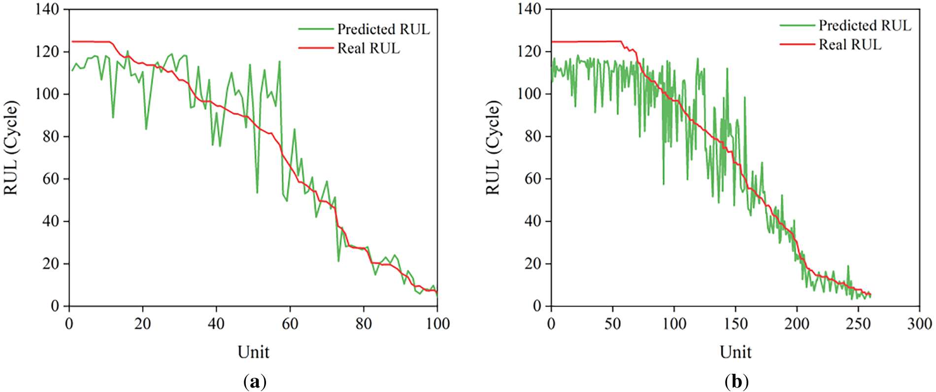
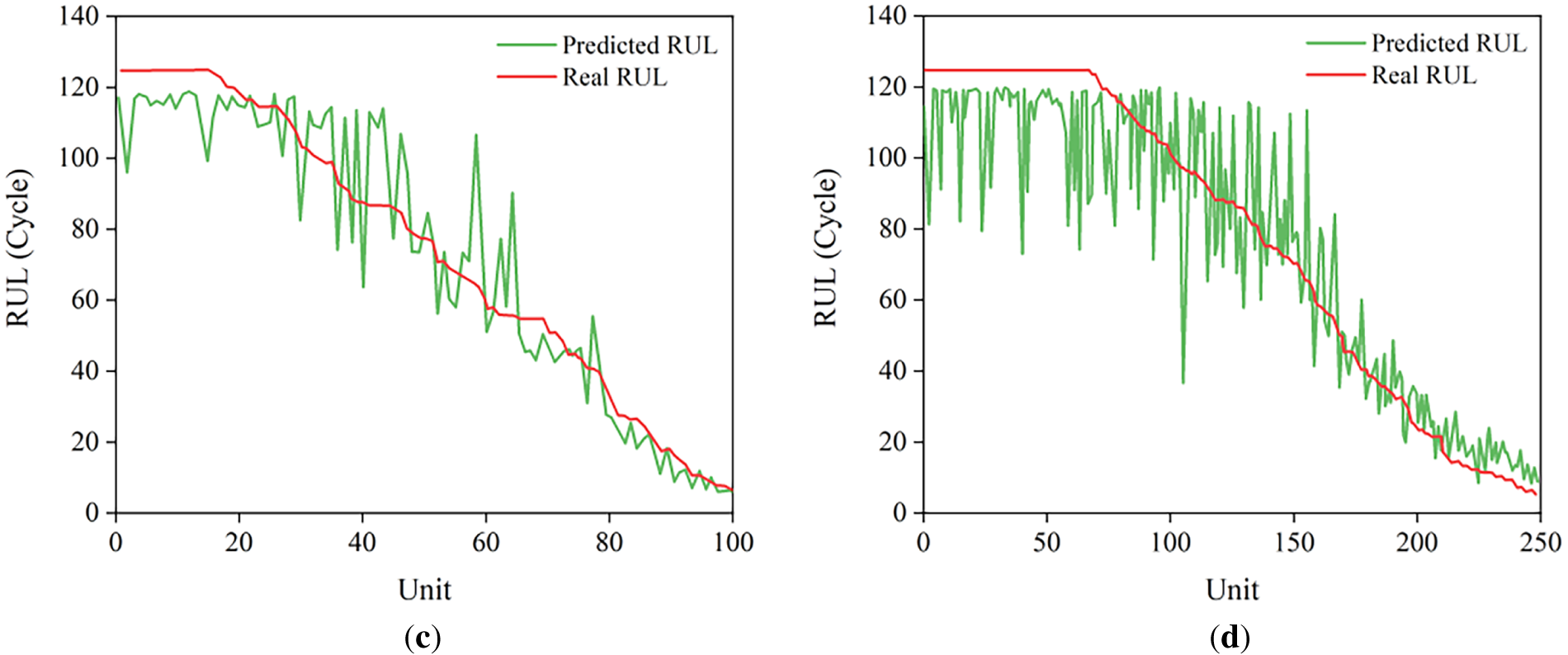
Figure 7: Comparison between real RUL and predicted RUL: (a) FD001; (b) FD002; (c) FD003; (d) FD004.

(2)   RUL interval probability prediction

In addition to point RUL predictions, the proposed MST-K model in this paper can also provide interval probability predictions for engine RUL. Fig. 8 shows the probability density functions of one engine each in the test sets of sub-datasets FD001 and FD002. Compared with point RUL predictions, interval probability predictions provide richer information and can effectively measure the probability of engine failure at every moment in the future, which is very important for ensuring flight safety and optimizing maintenance plans.

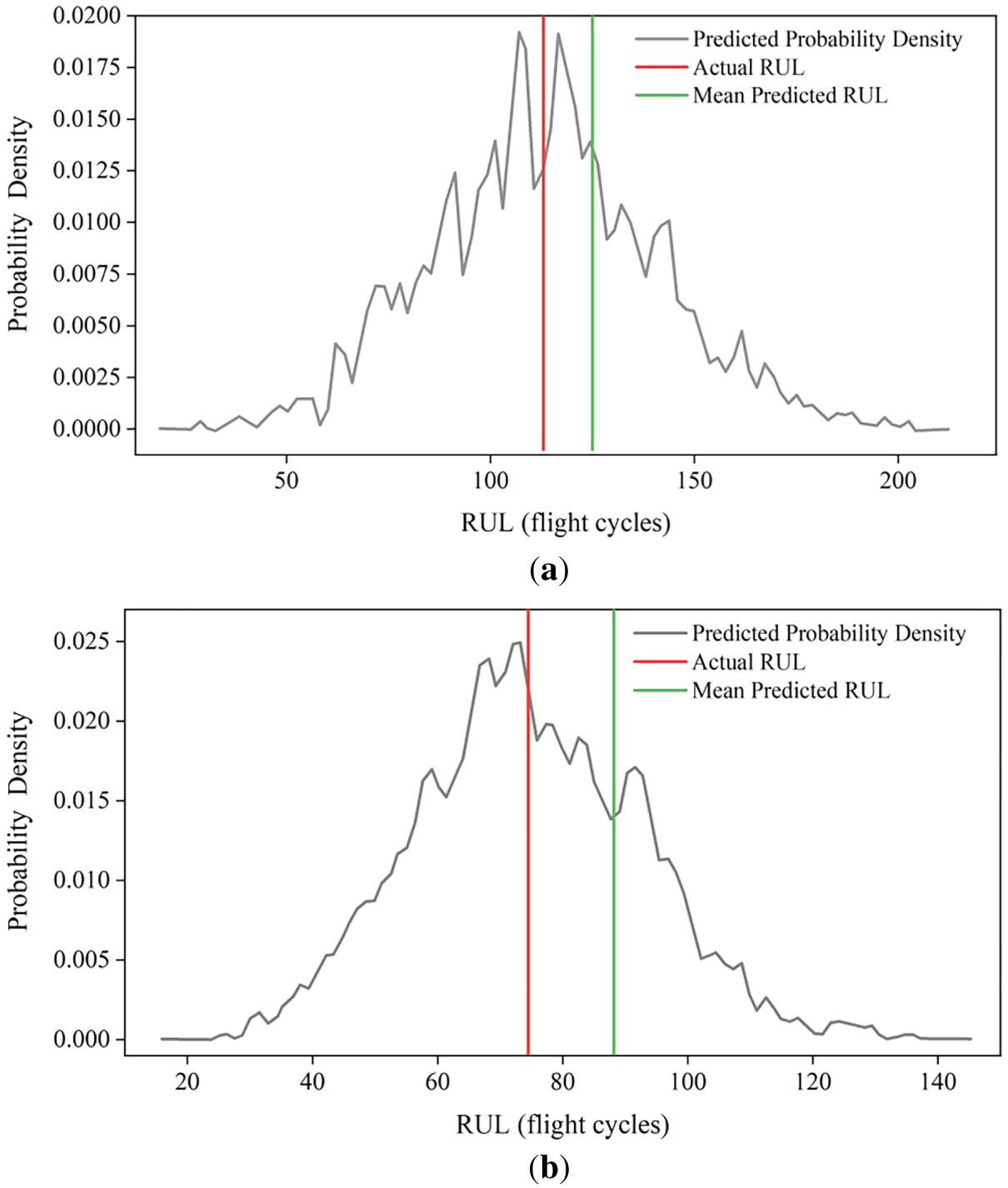
Figure 8: Probability density function of RUL for two engines: (a) test instance 6, data subset FD001 of CMAPSS; (b) test instance 25, data subset FD002 of CMAPSS.

Table 4 shows the values of α-Coverage when α∈{0.5,0.9,0.95}. It illustrates the practical significance of the α-Coverage value with an example of α=0.9. When α equals 0.9, the confidence interval [ri^0.5−0.5α,ri^0.5+0.5α] can be obtained according to Eq. (25), where ri^0.05 and ri^0.95 are the 5th percentile and the 95th percentile of the RUL prediction results, respectively. When α equals 0.9, after obtaining the confidence interval for each engine’s RUL in the test set, it can be determined whether the actual RUL falls within the confidence interval. For sub-dataset FD001, when α equals 0.9, the value of α-Coverage is 0.83, which means that the actual RUL of 83% of the engines falls within the confidence interval. This indicates that the uncertainty is slightly underestimated but is close to 90%, which is an acceptable result. From Table 4, it can be seen that the α-Coverage values for the RUL of engines in all sub-dataset test sets are close to the α value, indicating that the predicted probabilities match the observed results very well, thus the RUL interval probability prediction results obtained by the MST-K model are reliable. It can also be observed that when α=0.90 and α=0.95, the value of α-Mean width is large, that is, the average width of the confidence interval is large, indicating a higher level of predicted uncertainty. Fig. 9 further displays the α-Coverage curves corresponding to each sub-dataset when α∈{0,0.1,0.2,…,1}, showing that the α-Coverage curves of all four sub-datasets are close to the ideal curve, which again confirms that the MST-K model has well estimated the uncertainty of RUL prediction.

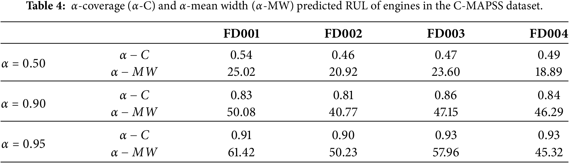
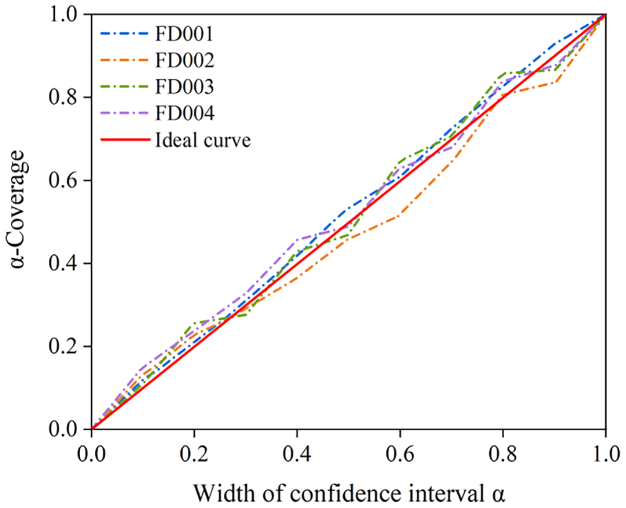
Figure 9: Credibility diagram of RUL interval probability prediction for the C-MAPSS.

(3)   Real-time RUL prediction

In the aforementioned analysis, the status information collection of the test set engines stops at a certain moment before the fault, meaning that the degradation data used is not complete, which limits the implementation of real-time RUL prediction. Fig. 10 shows the probability density functions of RUL obtained for Engine 1 in FD001 at actual RULs of 125, 75, and 25 flight cycles.

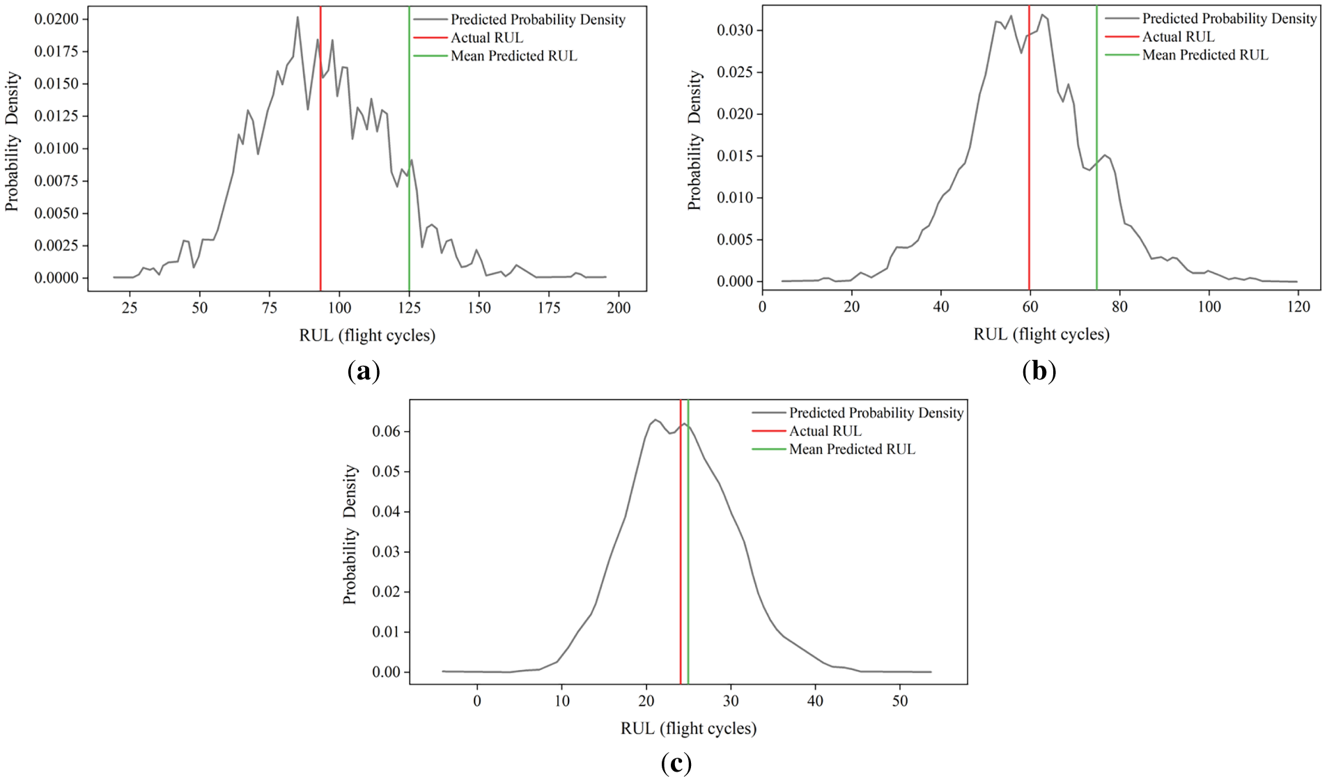
Figure 10: Probability density functions of RUL for engine 1 in FD001 at different flight cycles: (a) actual RUL = 125; (b) actual RUL = 75; (c) actual RUL = 25.

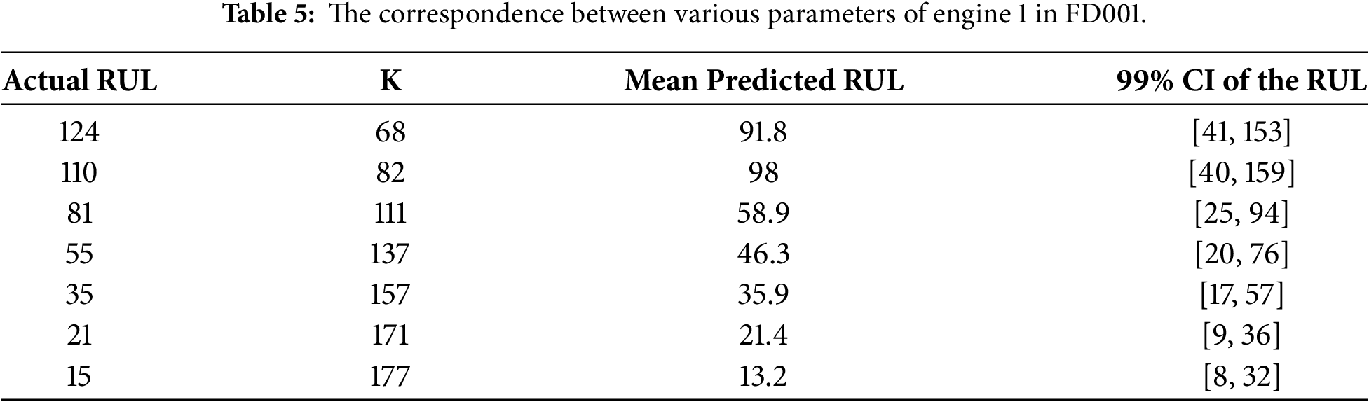
Fig. 11 displays the point predictions of RUL, as the collected condition monitoring data is not sufficient, leading to certain deviations in the predictions of the MST-K model. However, as the engine approaches failure and the condition monitoring data becomes richer. Table 5 means that if the procedure were repeated many times, 99% of such intervals would contain the true RUL. The interval [41, 153] is a 99% confidence interval for the RUL. This conclusion is more conducive to maintenance personnel making reasonable decisions about engine replacement.

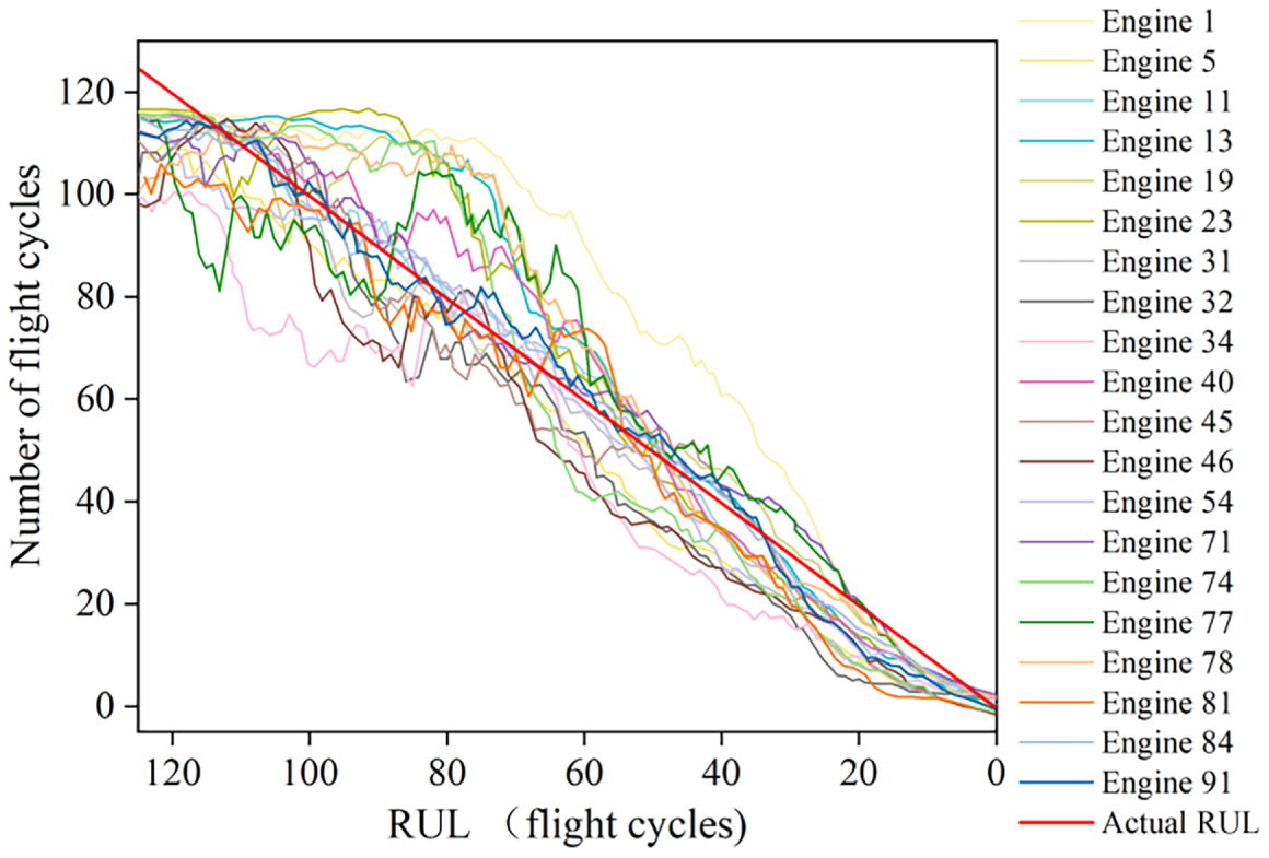
Figure 11: The average RUL of the last 125 flight cycles selected for real-time RUL prediction in FD001.

3.3 Ablation Study

Several strategies and components are proposed to adapt the MST-K model architecture for RUL prediction with multi-source time series data, including TDB, Koopman-GRU, and CILB. The results are shown in Table 6.

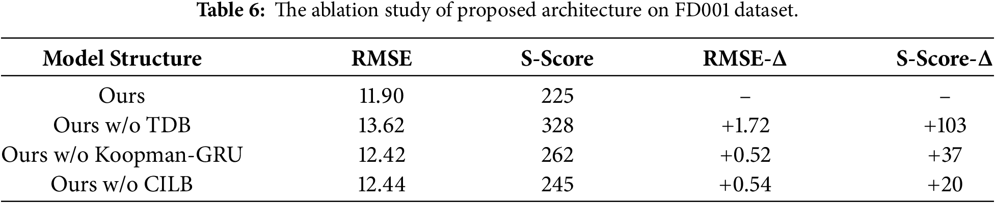
As shown in Table 6, when the TDB is removed, the RMSE increased by 1.72 and the S-score value increased by 103 on the FD001 dataset. This is primarily because, without the TDB, the model cannot effectively identify the stable degradation trends and unstable variations in the time series data, leading to a decrease in RUL prediction performance. When the Koopman-GRU module is removed, the RMSE increases by 0.52 and the S-score value increases by 37 on the FD001 dataset. This is mainly due to the model’s reduced ability to capture nonlinear dynamic features and local dependencies in the time series after the removal of the Koopman-GRU module, resulting in poorer RUL prediction outcomes. We conducted the sensitivity analysis on FD001, with all other hyperparameters fixed at their optimal values (batch size = 128, learning rate = 0.005, etc.). For each parameter configuration, we repeated the experiment 5 times with different random seeds and reported the mean RMSE and standard deviation. The GRU hidden size H determines the capacity of the recurrent network to capture temporal dependencies in the degradation signals. The observable vector used for Koopman lifting includes the GRU hidden state, so H simultaneously affects the Koopman mapping dimension. When the CILB is removed, the RMSE increased by 0.54 and the S-score value increased by 20 on the FD001 dataset. This is primarily because, without the CILB, the model cannot effectively model the dependencies between channels to generate the final channel feature representations, which reduces the model’s RUL prediction performance.

4  Conclusion

This paper introduces a spatiotemporal neural network for RUL prediction that integrates the Koopman operator with multivariate data fusion. The network structure includes a TDB that decomposes time series into trend and irregular components, a Koopman-GRU module for linear modeling of complex temporal dependency features in high-dimensional space, and a CILB to enhance feature expression capabilities. It also uses a combination of ensemble learning and KDE to obtain the probability density function of RUL, effectively measuring the uncertainty in RUL. The proposed method was applied to the C-MAPSS dataset and underwent RUL point prediction, interval probability prediction, real-time RUL prediction, and the ablation study.

(1) The MST-K model can effectively identify unstable changes in equipment performance degradation trends and enhance the comprehensive modeling capability of multivariate time series by capturing spatial features, thus outperforming other existing methods in RUL prediction. It ranks first in average performance across the four sub-datasets, with an RMSE value of 12.2675, which is 2.39 lower than the second-ranked GGCN method. The S-score value is 490.5, which is 333.25 lower than the second-ranked GGCN method. It also provides a good estimate of the uncertainty in RUL prediction.

(2) Real-time RUL prediction results indicate that the closer to the failure moment, the more accurate the RUL predictions of the MST-K model become, which is crucial for ensuring flight safety and optimizing maintenance plans.

(3) The ablation study confirms the necessity and effectiveness of each module in the proposed network architecture.

In future research, further consideration should be given to maintenance decision-making based on predictive information. Additionally, the effectiveness of the methods proposed in this paper should be tested on other types of sensor data, such as vibration signals and acoustic signals, to further expand the scope of model applicability.

Acknowledgement: Not applicable.

Funding Statement: The authors received no specific funding for this study.

Author Contributions: Conceptualization, Xinjian Gao and Zhonghua Cheng; methodology, Shizhuang Yin; software, Tielu Gao; validation, Yu Wang; formal analysis, Enzhi Dong; investigation, Enzhi Dong; resources, Xinjian Gao; data curation, Yu Wang; writing—original draft preparation, Xinjian Gao; writing—review and editing, Enzhi Dong; visualization, Xinjian Gao; supervision, Yu Wang; project administration, Zhonghua Cheng; funding acquisition, Tielu Gao. All authors reviewed and approved the final version of the manuscript.

Availability of Data and Materials: Not applicable.

Ethics Approval: Not applicable.

Conflicts of Interest: The authors declare no conflicts of interest.

References

1. Wang Y, Li Y, Zhang Y, Lei J, Yu Y, Zhang T, et al. Incorporating prior knowledge into self-supervised representation learning for long PHM signal. Reliab Eng Syst Saf. 2024;241:109602. doi:10.1016/j.ress.2023.109602. [Google Scholar] [CrossRef]

2. Yang S, Tang B, Wang W, Yang Q, Hu C. Physics-informed multi-state temporal frequency network for RUL prediction of rolling bearings. Reliab Eng Syst Saf. 2024;242:109716. doi:10.1016/j.ress.2023.109716. [Google Scholar] [CrossRef]

3. Wen M, Ibrahim MS, Meda AH, Zhang G, Fan J. In-situ early anomaly detection and remaining useful lifetime prediction for high-power white LEDs with distance and entropy-based long short-term memory recurrent neural networks. Expert Syst Appl. 2024;238:121832. doi:10.1016/j.eswa.2023.121832. [Google Scholar] [CrossRef]

4. Zhang Q, Liu Q, Ye Q. An attention-based temporal convolutional network method for predicting remaining useful life of aero-engine. Eng Appl Artif Intell. 2024;127:107241. doi:10.1016/j.engappai.2023.107241. [Google Scholar] [CrossRef]

5. Jiang K, Fan Y, Wen L, Xie ZG, Dong EZ, Zhu B, et al. Health status assessment of unmanned aerial vehicle engine based on AHP enhancement and multimodal fusion. Comput, Mater Continua. 2026;87(3):44. doi:10.32604/cmc.2026.077392. [Google Scholar] [CrossRef]

6. Guo J, Li D, Du B. A stacked ensemble method based on TCN and convolutional bi-directional GRU with multiple time windows for remaining useful life estimation. Appl Soft Comput. 2024;150:111071. doi:10.1016/j.asoc.2023.111071. [Google Scholar] [CrossRef]

7. Zhu B, Dong EZ, Cheng ZH, Jiang KX, Guo CM, Yue S. An integrated attention-BiLSTM approach for probabilistic remaining useful life prediction. Comput Mater Contin. 2026;87(1):38. doi:10.32604/cmc.2025.074009. [Google Scholar] [CrossRef]

8. Wang Y, Wang YB, Wen L, Li BY, Qin MZ, Li F, et al. Context-adaptive and physics-consistent constrained multimodal interpretable remaining useful life prediction. Comput Mater Contin. 2026;87(3):77. doi:10.32604/cmc.2026.077026. [Google Scholar] [CrossRef]

9. Duan F, Wang G. Bayesian analysis for the transformed exponential dispersion process with random effects. Reliab Eng Syst Saf. 2022;217:108104. doi:10.1016/j.ress.2021.108104. [Google Scholar] [CrossRef]

10. Yu W, Shao Y, Xu J, Mechefske C. An adaptive and generalized Wiener process model with a recursive filtering algorithm for remaining useful life estimation. Reliab Eng Syst Saf. 2022;217:108099. doi:10.1016/j.ress.2021.108099. [Google Scholar] [CrossRef]

11. Zhao YP, Chen YB. Extreme learning machine based transfer learning for aero engine fault diagnosis. Aerosp Sci Technol. 2022;121:107311. doi:10.1016/j.ast.2021.107311. [Google Scholar] [CrossRef]

12. Wang S, Tian J, Liang P, Xu X, Yu Z, Liu S, et al. Single and simultaneous fault diagnosis of gearbox via wavelet transform and improved deep residual network under imbalanced data. Eng Appl Artif Intell. 2024;133:108146. doi:10.1016/j.engappai.2024.108146. [Google Scholar] [CrossRef]

13. Liang P, Xu L, Shuai H, Yuan X, Wang B, Zhang L. Semisupervised subdomain adaptation graph convolutional network for fault transfer diagnosis of rotating machinery under time-varying speeds. IEEE ASME Trans Mechatron. 2024;29(1):730–41. doi:10.1109/tmech.2023.3292969. [Google Scholar] [CrossRef]

14. Shi J, Zhong J, Zhang Y, Xiao B, Xiao L, Zheng Y. A dual attention LSTM lightweight model based on exponential smoothing for remaining useful life prediction. Reliab Eng Syst Saf. 2024;243:109821. doi:10.1016/j.ress.2023.109821. [Google Scholar] [CrossRef]

15. Zhang J, Tian J, Li M, Leon JI, Franquelo LG, Luo H, et al. A parallel hybrid neural network with integration of spatial and temporal features for remaining useful life prediction in prognostics. IEEE Trans Instrum Meas. 2023;72:1–12. doi:10.1109/tim.2022.3227956. [Google Scholar] [CrossRef]

16. Yang H, Mei X, Jiang G, Tao T, Sun Z, Zhao F. Remaining useful life prediction of ball screw under time-varying conditions with limited data. IEEE ASME Trans Mechatron. 2022;27(5):4057–66. doi:10.1109/tmech.2022.3144351. [Google Scholar] [CrossRef]

17. Fu E, Hu Y, Peng K, Chu Y. Supervised contrastive learning based dual-mixer model for remaining useful life prediction. Reliab Eng Syst Saf. 2024;251:110398. doi:10.1016/j.ress.2024.110398. [Google Scholar] [CrossRef]

18. Cao Y, Ding Y, Jia M, Tian R. A novel temporal convolutional network with residual self-attention mechanism for remaining useful life prediction of rolling bearings. Reliab Eng Syst Saf. 2021;215:107813. doi:10.1016/j.ress.2021.107813. [Google Scholar] [CrossRef]

19. Xu Z, Zhang Y, Miao Q. An attention-based multi-scale temporal convolutional network for remaining useful life prediction. Reliab Eng Syst Saf. 2024;250:110288. doi:10.1016/j.ress.2024.110288. [Google Scholar] [CrossRef]

20. Fu S, Lin L, Wang Y, Guo F, Zhao M, Zhong B, et al. MCA-DTCN: a novel dual-task temporal convolutional network with multi-channel attention for first prediction time detection and remaining useful life prediction. Reliab Eng Syst Saf. 2024;241:109696. doi:10.1016/j.ress.2023.109696. [Google Scholar] [CrossRef]

21. Chang Y, Chen J, Lv H, Liu S. Heterogeneous bi-directional recurrent neural network combining fusion health indicator for predictive analytics of rotating machinery. ISA Trans. 2022;122:409–23. doi:10.1016/j.isatra.2021.04.024. [Google Scholar] [CrossRef]

22. Gao S, Xiong X, Zhou Y, Zhang J. Bearing remaining useful life prediction based on a scaled health indicator and a LSTM model with attention mechanism. Machines. 2021;9(10):238. doi:10.3390/machines9100238. [Google Scholar] [CrossRef]

23. Yu Y, Si X, Hu C, Zhang J. A review of recurrent neural networks: LSTM cells and network architectures. Neural Comput. 2019;31(7):1235–70. doi:10.1162/neco_a_01199. [Google Scholar] [CrossRef]

24. Shao Z, Wang F, Xu Y, Wei W, Yu C, Zhang Z, et al. Exploring progress in multivariate time series forecasting: comprehensive benchmarking and heterogeneity analysis. arXiv:2310.06119. 2023. doi:10.48550/arXiv.2310.06119. [Google Scholar] [CrossRef]

25. Wu HX, Xu JH, Wang JM, Long M. Autoformer: decomposition transformers with auto-correlation for long-term series forecasting. Adv Neural Inf Process Syst. 2021;34:22419–30. [Google Scholar]

26. Zeng A, Chen M, Zhang L, Xu Q. Are transformers effective for time series forecasting? Proc AAAI Conf Artif Intell. 2023;37(9):11121–8. doi:10.1609/aaai.v37i9.26317. [Google Scholar] [CrossRef]

27. Han L, Chen XY, Ye HJ, Zhan DC. SOFTS: efficient multivariate time series forecasting with series-core fusion. arXiv:2404.14197. 2024. doi:10.48550/arXiv.2404.14197. [Google Scholar] [CrossRef]

28. Saxena A, Goebel K. Turbofan engine degradation simulation data set. Moffett Field, CA, USA: NASA Ames Prognostics Data Repository; 2008. p. 878–87. [cited 2026 May 01]. Available from: http://ti.arc.nasa.gov/project/prognostic-data-repository. [Google Scholar]

29. Wu Y, Yuan M, Dong S, Lin L, Liu Y. Remaining useful life estimation of engineered systems using Vanilla LSTM neural networks. Neurocomputing. 2018;275:167–79. doi:10.1016/j.neucom.2017.05.063. [Google Scholar] [CrossRef]

30. Costa N, Sánchez L. Variational encoding approach for interpretable assessment of remaining useful life estimation. Reliab Eng Syst Saf. 2022;222:108353. doi:10.1016/j.ress.2022.108353. [Google Scholar] [CrossRef]

31. Miao H, Li B, Sun C, Liu J. Joint learning of degradation assessment and RUL prediction for aeroengines via dual-task deep LSTM networks. IEEE Trans Ind Inf. 2019;15(9):5023–32. doi:10.1109/tii.2019.2900295. [Google Scholar] [CrossRef]

32. Li Y, Chen Y, Hu Z, Zhang H. Remaining useful life prediction of aero-engine enabled by fusing knowledge and deep learning models. Reliab Eng Syst Saf. 2023;229:108869. doi:10.1016/j.ress.2022.108869. [Google Scholar] [CrossRef]

33. Mitici M, de Pater I, Barros A, Zeng Z. Dynamic predictive maintenance for multiple components using data-driven probabilistic RUL prognostics: the case of turbofan engines. Reliab Eng Syst Saf. 2023;234:109199. doi:10.1016/j.ress.2023.109199. [Google Scholar] [CrossRef]

34. De Pater I, Mitici M. Novel metrics to evaluate probabilistic remaining useful life prognostics with applications to turbofan engines. PHM Soc Eur Conf. 2022;7(1):96–109. doi:10.36001/phme.2022.v7i1.3320. [Google Scholar] [CrossRef]

35. Fan L, Chai Y, Chen X. Trend attention fully convolutional network for remaining useful life estimation. Reliab Eng Syst Saf. 2022;225:108590. doi:10.1016/j.ress.2022.108590. [Google Scholar] [CrossRef]

36. Li T, Zhou Z, Li S, Sun C, Yan R, Chen X. The emerging graph neural networks for intelligent fault diagnostics and prognostics: a guideline and a benchmark study. Mech Syst Signal Process. 2022;168:108653. doi:10.1016/j.ymssp.2021.108653. [Google Scholar] [CrossRef]

37. Wang L, Cao H, Xu H, Liu H. A gated graph convolutional network with multi-sensor signals for remaining useful life prediction. Knowl Based Syst. 2022;252:109340. doi:10.1016/j.knosys.2022.109340. [Google Scholar] [CrossRef]

38. Zhang J, Li X, Tian J, Luo H, Yin S. An integrated multi-head dual sparse self-attention network for remaining useful life prediction. Reliab Eng Syst Saf. 2023;233:109096. doi:10.1016/j.ress.2023.109096. [Google Scholar] [CrossRef]

39. Zhao K, Jia Z, Jia F, Shao H. Multi-scale integrated deep self-attention network for predicting remaining useful life of aero-engine. Eng Appl Artif Intell. 2023;120:105860. doi:10.1016/j.engappai.2023.105860. [Google Scholar] [CrossRef]