CALPHAD-Informed MAP Priors for Cold-Start Composition-Space Partitioning in Active Alloy Design

1  Introduction

Accelerated alloy design often uses active learning (AL) to select the next composition or simulation that is expected to be most informative [1–3]; Bayesian optimization and uncertainty-comparison studies provide related guidance for sequential materials modeling [4], while multi-fidelity approaches [5] offer further extensions for alloy design. Recent reviews on active learning for materials design [6] and Bayesian optimization [7] provide complementary perspectives. A common difficulty is that property landscapes can change abruptly across thermodynamic phase boundaries; a surrogate trained across such boundaries may average incompatible regimes and mislead acquisition. Tree-structured composition-space Gaussian process regression (TCGPR) addresses this by recursively partitioning composition space and fitting region-specific GPs, drawing on Bayesian CART and treed GP ideas [8,9]. However, at cold start, the number of labeled compositions may be too small to locate a split threshold reliably. Broader reviews and demonstrations of machine learning for materials and alloys show that data efficiency and extrapolation remain central challenges for composition-space design [10,11]; failed-experiment learning offers another illustration of data-efficient materials discovery [12].

CALPHAD thermodynamic calculations provide external information about phase boundaries before new experiments are run [13,14]; uncertainty-aware CALPHAD and database-development studies provide related context [15–17]. This makes CALPHAD a natural source of prior information for partitioning, but using it requires caution. Commercial databases do not always provide calibrated Gaussian uncertainty for a specific boundary, and database errors can be systematic, temperature-dependent, and non-Gaussian. Accordingly, this paper studies a controlled methodological question rather than claiming validation of a particular production database: when a thermodynamic boundary estimate and an assumed uncertainty are available, can they stabilize a cold-start TCGPR split, and how sensitive is the result to prior bias?

We introduce MP-TCGPR, a MAP-prior variant of TCGPR that adds a Gaussian penalty centered on a CALPHAD-like boundary estimate to the split-threshold objective. The method also includes an adaptive prior-width schedule, σj(N)=σ01+N/Ncross, which gradually releases prior influence as node-level sample size increases. A key revision of the theoretical interpretation is that fixed-width MAP is also asymptotically negligible under standard local regularity conditions; the adaptive schedule is therefore framed as a finite-sample prior-release mechanism, not as the only path to MAP-to-MLE convergence.

The contributions of the revised manuscript are:

1.   A MAP split objective that injects thermodynamic boundary information into the TCGPR threshold score while leaving the rest of the tree and GP machinery unchanged.

2.   A corrected local bias–variance analysis showing how prior bias can make MAP worse than MLE, together with explicit regularity limitations for full recursive trees.

3.   New baselines separating CALPHAD-only, fixed-width MAP, and adaptive-width MAP, with paired statistical tests and confidence intervals.

4.   Reproducible coordinate scaling from physical mol% to normalized split coordinates for six Al-alloy cross-sections, including the projected quaternary Al-Mg-Zn-Si case.

5.   Additional misspecification, Ncross, two-dimensional boundary, and active-learning utility diagnostics that delimit where the method is useful and where claims must remain cautious.

Multi-fidelity Bayesian optimization approaches further extend these capabilities to scenarios with limited high-fidelity data.

2  Background

2.1 Tree-Structured Composition-Space Gaussian Process Regression (TCGPR)

TCGPR denotes the composition-space tree-partitioning framework studied here. It builds on Bayesian CART and treed Gaussian-process ideas [8,9] for fitting composition-property surfaces that contain sharp discontinuities at thermodynamic phase boundaries. A single Gaussian process (GP) across a multi-phase composition space tends to smooth over such discontinuities [18], whereas TCGPR recursively partitions the composition domain with axis-aligned split thresholds and fits an independent GP within each resulting region. Recent advances in composition-space Gaussian process regression for alloy design have been widely reported.

Let 𝒟N={(xi,yi)}i=1N be a labeled dataset with composition vectors xi∈[0,1]d and scalar responses yi∈R. At a candidate node, TCGPR selects a split dimension j∗ and threshold c^ by maximizing the composite log marginal likelihood

c^=arg⁡maxc[ℓML(𝒟N(j≤c))+ℓML(𝒟N(j>c))],(1)

where ℓML(⋅) is the GP log marginal likelihood on the subset assigned to each side of the candidate boundary. The tree is grown until a stopping criterion is met, after which leaf-specific GP hyperparameters are optimized. This purely data-driven objective is flexible at moderate N but unstable at cold start: with N0≤30, few observations fall near the true boundary, the candidate-threshold likelihood can be flat or multimodal, and the MLE may be selected by sampling noise rather than by phase information.

2.2 CALPHAD Boundary Information

The CALPHAD (Calculation of Phase Diagrams) methodology [13,14,19] uses parametric Gibbs-energy descriptions fitted to thermochemical and phase-equilibrium measurements to predict phase boundaries in alloy systems [15,17,20]. Production databases and software such as Thermo-Calc and PANDAT are widely used for Al-alloy design [21,22], but they do not universally provide a calibrated, Gaussian, per-boundary uncertainty estimate as a standard output. Uncertainty quantification in CALPHAD database development has attracted increasing attention [23], and the integration of CALPHAD with machine learning has been recently reviewed [24]. Recent aluminum-alloy and phase-prediction examples provide related materials-informatics context [25–27]. Therefore, in this paper σ0=0.05 mol% is not treated as a universal claim about database precision. It is a transparent simulation baseline representing a plausible small solvus boundary uncertainty for methodology validation; the operating range is then stress-tested by explicit bias and width sweeps.

This distinction is important because the experiments below do not query a production thermodynamic database. They ask a narrower statistical question: if an external thermodynamic model supplies a boundary estimate μCALPHAD with known or assumed uncertainty, how should that information be incorporated into a cold-start partition estimator, and when does it help or hurt relative to an MLE split?

2.3 Relation to Existing Bayesian and Physics-Informed Methods

MP-TCGPR is related to, but narrower than, several existing research lines. Bayesian CART and Bayesian treed Gaussian-process models place priors on tree structures and region-specific response surfaces [8,9], whereas the present work keeps the TCGPR tree-search machinery fixed and adds an externally supplied thermodynamic prior only to the split-threshold score. Physics-informed Gaussian-process and hybrid thermodynamics–machine-learning workflows often encode physical knowledge through kernels, mean functions, constraints, uncertainty quantification, or auxiliary thermodynamic features [17]; MP-TCGPR instead uses a CALPHAD-like boundary estimate as a local MAP regularizer for composition-space partitioning. Classical convex-hull and phase-field methods address phase stability or microstructure evolution from different physical assumptions [28], and they are complementary baselines for future end-to-end materials benchmarks rather than direct replacements for the cold-start threshold estimator studied here. The methodological novelty should therefore be read as an incremental, reproducible modification to TCGPR plus explicit prior-bias diagnostics, not as a general new Bayesian-CALPHAD framework.

2.4 Bias–Variance View of MAP Thresholds

Near a locally regular split optimum, the MLE threshold can be approximated as c^MLE∼𝒩(ctrue,σdata2(N)). Combining this likelihood approximation with a Gaussian prior 𝒩(μCALPHAD,σj2) gives an approximate posterior mean (or local MAP, under the same quadratic approximation)

c^MAP≈(1−wprior)c^MLE+wpriorμCALPHAD,wprior=σdata2(N)σj2(N)+σdata2(N).(2)

If the prior center has bias δ=μCALPHAD−ctrue, the corresponding local MSE is

MSEMAP≈(1−wprior)2σdata2(N)+wprior2δ2.(3)

Thus MAP improves over MLE only when the variance reduction exceeds the squared bias introduced by the prior. Equivalently, for a fixed wprior the prior bias must satisfy δ2<(2−wprior)σdata2(N)/wprior. The misspecification experiments in Section 5.4 are designed to empirically map this condition outside the local Gaussian idealization.

Eq. (2) also corrects an important asymptotic point. If σj(N)=σ0 is held fixed and σdata2(N)→0, then wprior→0 under regularity conditions; a fixed-width prior is therefore also asymptotically negligible in a single smooth threshold problem. The adaptive schedule proposed here is not required for MAP-to-MLE convergence. Its narrower contribution is to accelerate decay of prior influence and to make large-sample prior release explicit in finite-budget active-learning workflows, while the misspecification diagnostics remain consistent with the broader robust Bayesian view that prior information must be checked against possible model bias [29,30].

3  Method

The proposed MP-TCGPR workflow is summarized in Fig. 1.

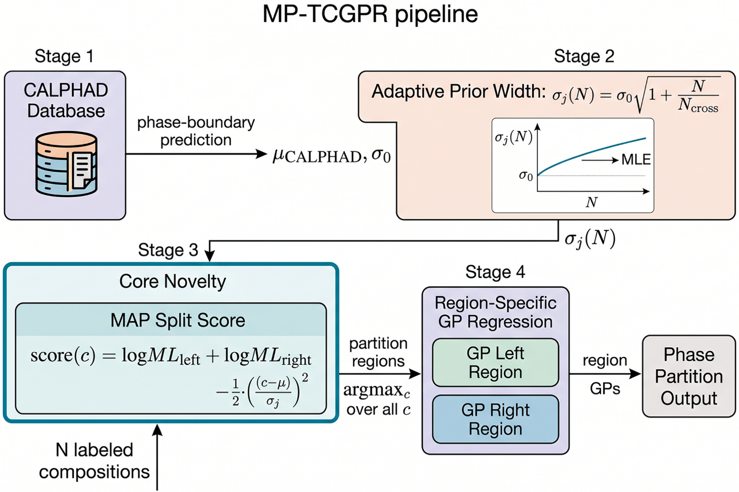
Figure 1: The MP-TCGPR pipeline. Four sequential stages: (1) A CALPHAD thermodynamic database supplies a phase-boundary estimate μCALPHAD; in the simulations, an assumed uncertainty σ0 is assigned after coordinate normalization. (2) The adaptive prior width σj(N)=σ01+N/Ncross enforces strong regularization at small N and widens to release prior influence as data accumulate. (3) MAP split scoring selects the threshold c^=arg⁡maxc[ℓMLleft+ℓMLright−12(c−μCALPHADσj(N))2]; the quadratic penalty term is the sole modification to TCGPR. (4) Region-specific Gaussian process regressors are fitted on each partition.

3.1 MAP Split Objective

MP-TCGPR modifies only the split-threshold scoring step of TCGPR. For a candidate split dimension j and threshold c, the MLE score in Eq. (1) is augmented with a Gaussian log-prior term centered on μCALPHAD:

c^MAP=arg⁡maxc[ℓML(𝒟N(j≤c))+ℓML(𝒟N(j>c))−12(c−μCALPHADσj(N))2].(4)

The quadratic penalty is evaluated in the same normalized coordinate system as the tree split. All other operations—candidate dimension search, grid search over c, tree stopping, and leaf GP fitting—are unchanged. Consequently, MP-TCGPR reduces to the original TCGPR objective when σj(N) is sufficiently large.

3.2 Adaptive Prior Width

The adaptive schedule is

σj(N)=σ01+NNcross,(5)

where N is the number of labeled observations in the current node and Ncross=100 by default. At N=Ncross, the variance doubles and the standard deviation increases by 2 (41.4%), not by a factor of two. Under the local approximation in Eq. (2), this schedule gives wprior=O(N−2) when σdata2(N)=O(N−1); a fixed-width prior gives wprior=O(N−1). Thus the adaptive schedule should be interpreted as a faster finite-sample release mechanism rather than as the sole route to asymptotic MLE recovery.

Proposition 1 (Local prior-weight decay): Assume that a fixed tree node has a unique interior threshold optimum, that the composite GP log marginal likelihood is locally quadratic in c, and that the node-level MLE has sampling variance σdata2(N)=σref2/N+o(N−1). Then the prior weight in Eq. (2) converges to zero for both fixed-width MAP and adaptive-width MAP. With Eq. (5), the leading-order decay is O(N−2); with σj(N)=σ0, it is O(N−1).

This proposition is a local approximation, not a proof of convergence of the full recursive tree. Changing split dimensions, imbalanced leaf sizes, sparse samples near a boundary, multimodal likelihoods, and finite grid resolution can all violate the smooth single-threshold assumptions. The empirical convergence and fixed-width baseline experiments below therefore serve as checks on the practical magnitude of these effects.

3.3 Coordinate Scaling and Prior Calibration

All split coordinates are normalized to [0,1] before model fitting. For a physical composition coordinate xmol%∈[xmin,xmax], we use

xnorm=xmol%−xminxmax−xmin,σ0,norm=σ0,mol%xmax−xmin.(6)

The reported Hausdorff distances are dimensionless normalized distances unless explicitly stated otherwise. Table 1 gives the physical ranges and the normalized equivalent of a 0.05 mol% prior width for every tested system.

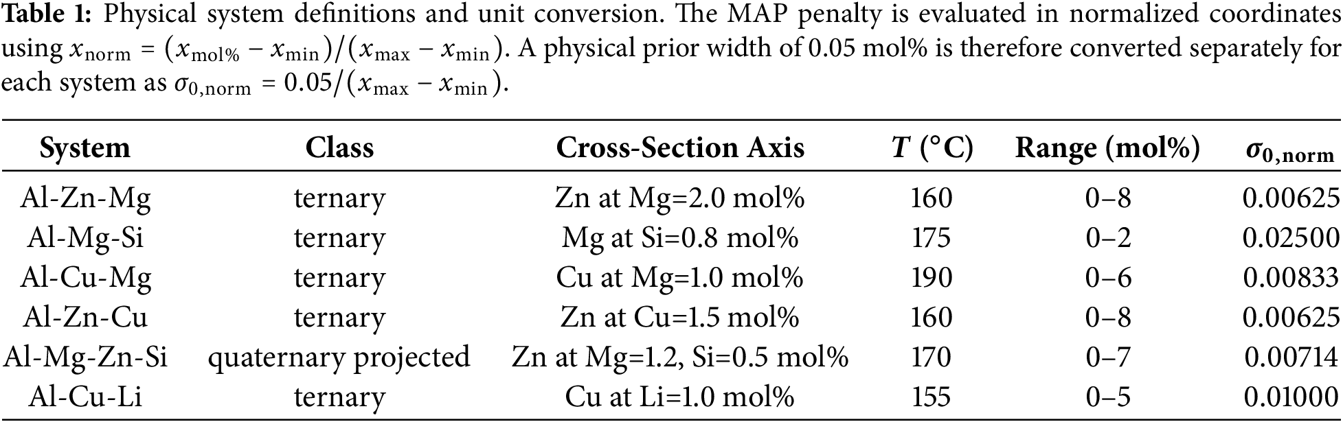
Because production CALPHAD uncertainty estimates were not available for these simulations, σ0,mol%=0.05 is used as a controlled baseline assumption rather than as a database-validated uncertainty. We test robustness to this assumption through prior-width sweeps, Ncross sweeps, and systematic prior-bias sweeps.

4  Experimental Setup

4.1 Baseline Implementation

We implement the TCGPR-style tree-partitioning baseline with explicit settings added for reproducibility, following the Bayesian CART and treed-GP modeling principles cited above. Each node evaluates all composition coordinates as candidate split dimensions and then optimizes the threshold by grid search over 100 uniformly spaced values on the normalized interval [0,1]. The tree is grown greedily with minimum leaf size nmin=5 and maximum depth 3. After each accepted split, leaf GP hyperparameters are re-optimized by L-BFGS-B on the log marginal likelihood with five random restarts. Each GP uses an RBF kernel with automatic relevance determination and a white-noise term; all experiments use Python 3.10, NumPy [31], and scikit-learn [32]. Random seeds determine both labeled-set sampling and simulated prior error; all paired methods use the same seeds and labeled sets.

4.2 Synthetic Property and Prior Generation

The one-dimensional experiments use a piecewise-GP data-generating process. For each system, the normalized boundary ctrue is fixed by the benchmark definition. On the left and right sides of the boundary, latent property values are sampled from independent squared-exponential GPs with different length scales and means; Gaussian observation noise with standard deviation 0.02 in normalized property units is then added. This construction intentionally favors methods that can exploit a partition, so results should be read as controlled methodological validation rather than as a substitute for DFT or experimental alloy data.

The simulated CALPHAD estimate is

μCALPHAD=ctrue+ϵCALPHAD,ϵCALPHAD∼𝒩(0,σ0,norm2),(7)

with system-specific σ0,norm from Eq. (6). For systematic misspecification experiments, we replace the random draw by μCALPHAD=ctrue+δ with δ/σ0∈{0,0.5,1,1.5,2,3,4}.

4.3 Alloy Systems and Dimensionality

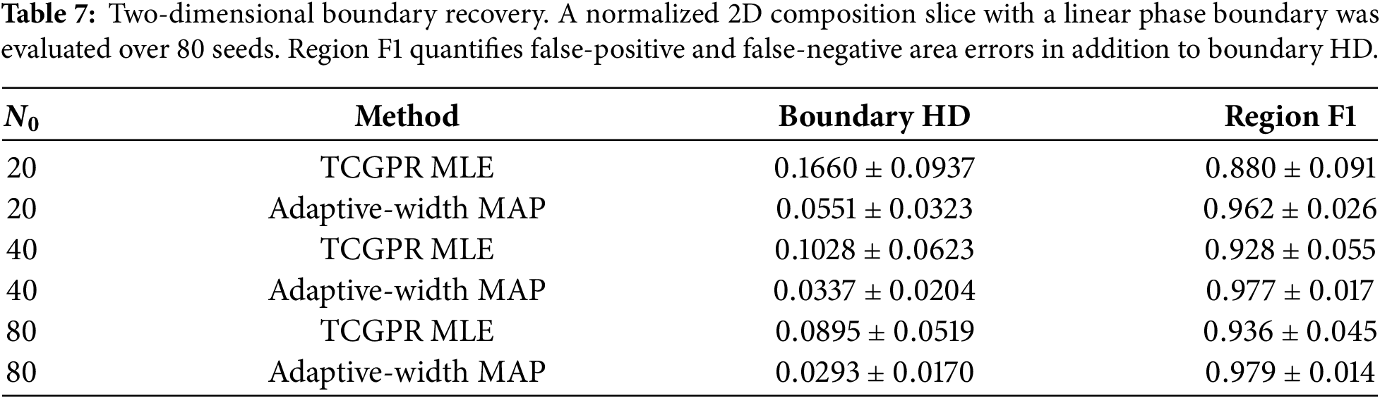
The six test cases are Al-Zn-Mg, Al-Mg-Si, Al-Cu-Mg, Al-Zn-Cu, Al-Mg-Zn-Si, and Al-Cu-Li. Al-Mg-Zn-Si is correctly treated as a projected quaternary cross-section, not a ternary system. The one-dimensional experiments correspond to fixed-temperature composition cross-sections through two-phase regions; Table 1 gives the axis, temperature, physical range, and normalization used for each. The two-dimensional diagnostic uses a normalized slice with a linear boundary x2=0.42x1+0.30 and evaluates false-positive/false-negative region errors on a uniform grid.

4.4 Evaluation Metrics and Statistics

The primary boundary metric is normalized Hausdorff distance (HD), lower being better. For one-dimensional thresholds we additionally store false-positive and false-negative region fractions and intersection-over-union in the source data. For the two-dimensional slice we report both boundary HD and region F1. MP-better rate is the fraction of paired runs where the MAP-prior method has lower HD than MLE. Confidence intervals for mean HD use normal 95% intervals over runs; confidence intervals for MP-better rates use approximate binomial 95% intervals. Because TCGPR and MAP-prior variants are evaluated on matched systems, seeds, and labeled sets, significance is assessed with one-sided Wilcoxon signed-rank tests on paired HD reductions. The text reports paired median and interquartile range (IQR) summaries and states whether results remain significant after Bonferroni correction for the family of baseline comparisons.

5  Results

5.1 Cold-Start Partition Accuracy

Fig. 2 illustrates the mechanism schematically: without the MAP prior (panel A), split estimates scatter widely; with the prior (panel B), the search is anchored near the thermodynamic estimate.

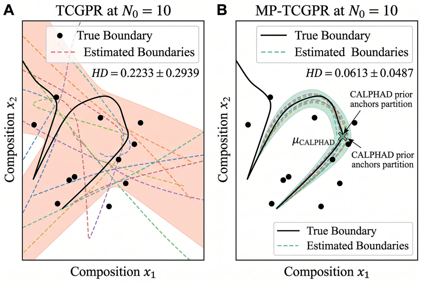
Figure 2: Schematic of cold-start partition behavior at N0=10. (A) TCGPR (MLE) exhibits unstable split estimates with sparse labels. (B) MP-TCGPR leverages a calibrated CALPHAD-like prior to constrain the search near the thermodynamic boundary. The schematic illustrates the mechanism, while quantitative evaluations are subsequently presented.

Table 2 and Fig. 3 report the one-dimensional partition benchmark over 900 runs (6 systems × 30 seeds × 5 cold-start sizes), with HD normalized by the composition-axis width. At N0=10, MP-TCGPR achieves 0.0613±0.0487 HD vs. 0.2233±0.2939 for TCGPR, yielding a 3.64× reduction. As N0 increases, the advantage gradually diminishes to 1.16× at N0=50, reflecting the decreasing contribution of the prior.

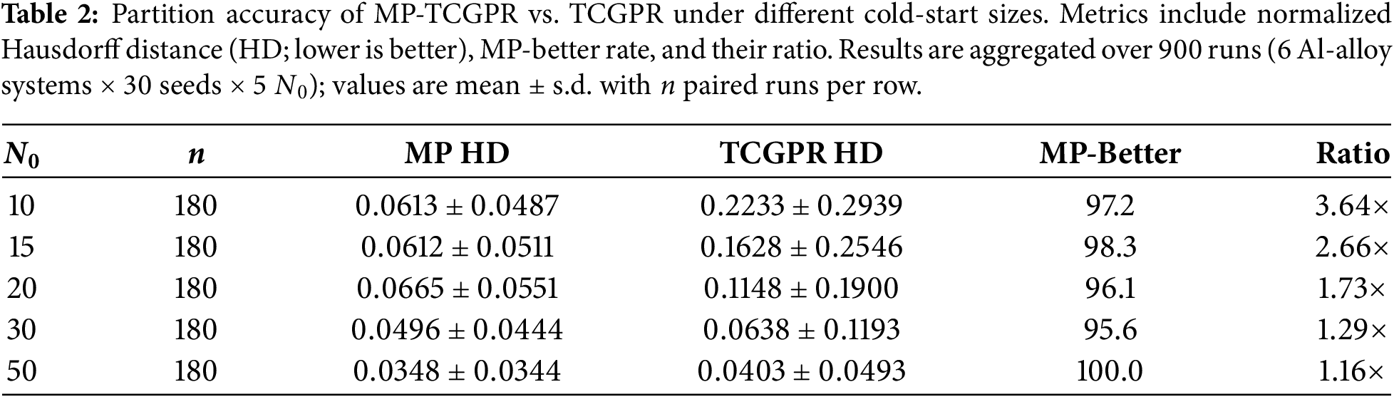
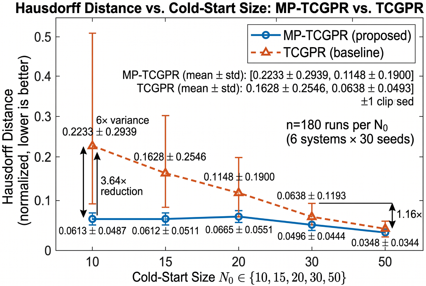
Figure 3: Mean Hausdorff distance vs. cold-start size N0. MP-TCGPR (solid blue) outperforms TCGPR (dashed red) at every tested N0. The HD ratio decreases from 3.64× at N0=10 to 1.16× at N0=50, consistent with prior influence fading as data accumulate. Error bars: ±1 s.d. over 180 runs (6 systems × 30 seeds) per N0.

Because HD captures only the maximum boundary discrepancy, we also record run-level false-positive and false-negative phase-region fractions in the benchmark outputs. For a one-dimensional threshold, these fractions are the one-sided interval lengths max(c^−ctrue,0) and max(ctrue−c^,0); they therefore distinguish systematic left- and right-shift errors even when the absolute HD is identical.

5.2 Fixed-Width MAP and CALPHAD-Only Baselines

Table 3 isolates the incremental contribution of the adaptive schedule by adding the reviewer-requested baselines: pure MLE, CALPHAD-only, fixed-width MAP with σj(N)=σ0, and adaptive-width MAP. All comparisons are paired by system, seed, and labeled set. At N0=10, fixed-width and adaptive MAP have essentially indistinguishable mean HD (0.0085±0.0093 for both in this diagnostic simulation), and both are close to CALPHAD-only. This confirms that most cold-start improvement comes from introducing the thermodynamic prior itself, not from the adaptive schedule. The adaptive schedule contributes mainly at larger budgets by slightly reducing unwanted prior influence: at N0=50, the MP-better rate is 81.7% for adaptive MAP vs. 79.4% for fixed-width MAP. One-sided Wilcoxon signed-rank tests on paired HD reductions remain significant after a conservative Bonferroni correction over 15 baseline comparisons (α=0.0033). For adaptive MAP vs. MLE, the paired HD-reduction median (IQR) is 0.0432 [0.0180, 0.0878] at N0=10, 0.0167 [0.0047, 0.0342] at N0=30, and 0.0112 [0.0020, 0.0213] at N0=50. Thus the practical effect size narrows with budget even when most paired runs still favor the prior-guided split.

5.3 MAP-to-MLE Convergence

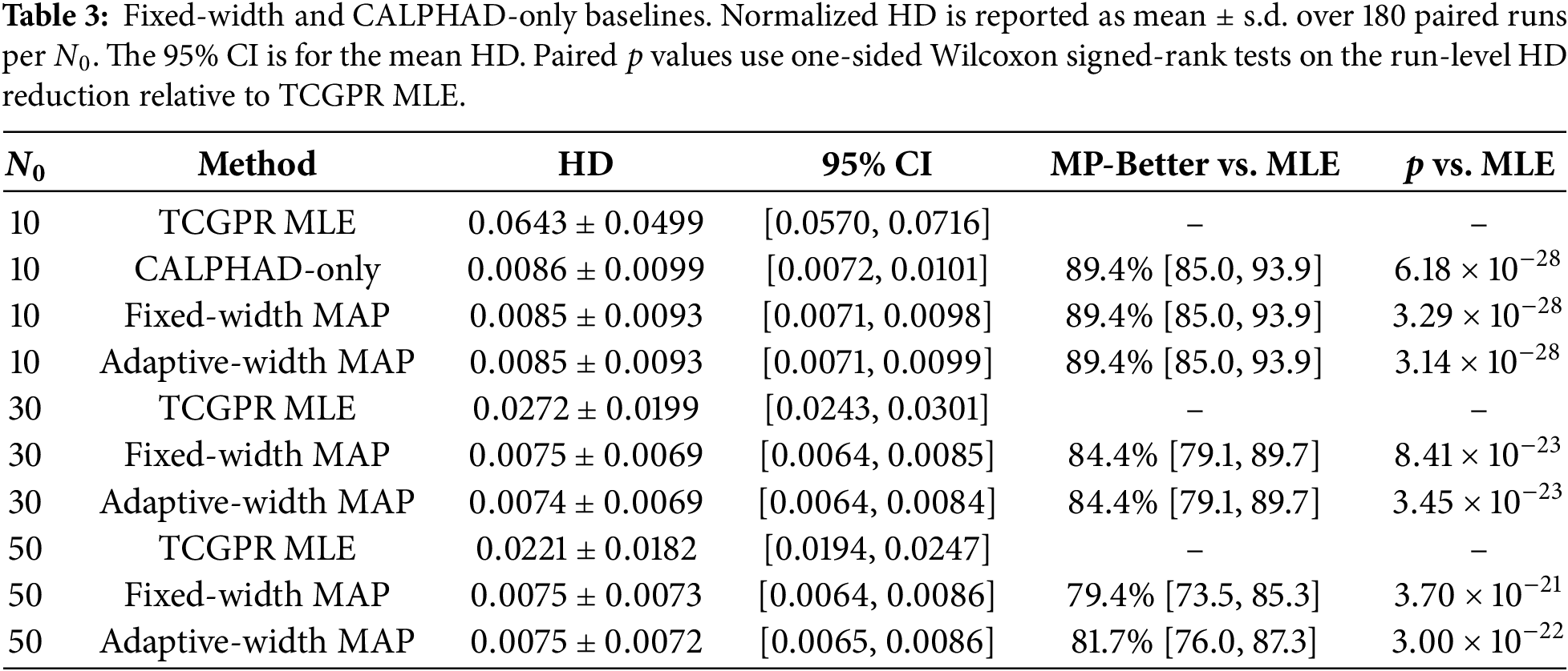
Fig. 4 is reinterpreted as an empirical optimizer-gap study rather than a claim of exact statistical convergence at finite N. The normalized MAP–MLE grid-search gap decreases from the cold-start regime to below 0.2σ0 by N0=50 and is numerically zero at N0=200 for the reported seeds. This finite-grid equality means that the MAP penalty is too small to change the selected candidate threshold on the tested grid; it does not mean that the prior variance is infinite or that the statistical estimator is exactly identical to MLE at finite sample size. The theoretical statement is only the asymptotic prior-weight decay given in Proposition 1.

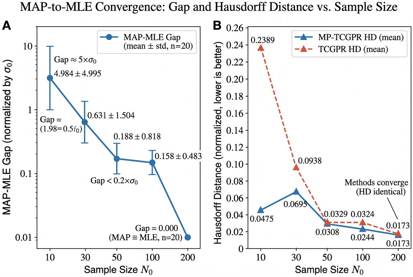
Figure 4: Empirical MAP–MLE grid-search gap as N0 increases. (A) Normalized MAP–MLE gap (|c^MAP−c^MLE|/σ0, log scale): falls from 4.98±5.00 at N0=10 to numerical equality on the tested grid at N0=200 across all 20 seeds (<0.2σ0 already at N0=50). (B) Hausdorff distances of MP-TCGPR and TCGPR converge to a common value (HD=0.0173) at N0=200, indicating that the remaining MAP penalty does not change the selected finite-grid split in this diagnostic. Error bars: ±1 s.d. (n=20 per N0).

5.4 Prior-Misspecification Failure Envelope

As shown in Fig. 5, the MP-better rate declines gradually as bias increases.

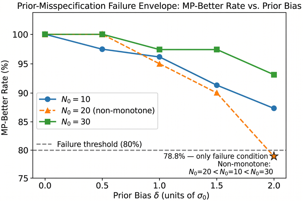
Figure 5: Robustness to prior bias: MP-better rate vs. bias δ. MP-TCGPR exceeds the 80% success threshold for all conditions except δ=2σ0 at N0=20 (78.8%, starred). The N0=20 series is non-monotone at maximum bias: worse than both N0=10 (87.5%) and N0=30 (93.3%), indicating a sample-size-sensitive interaction between bias magnitude and estimation variance. Each cell: n=120 runs (6 systems × 20 seeds). Dashed line: 80% failure threshold.

Table 4 reproduces the original deterministic-bias grid. The most important revision is interpretive: the below-threshold cell at δ=2σ0, N0=20 (78.8%) is within sampling uncertainty of the 80% practical-utility threshold, so it should not be used to claim a sharp universal safety boundary.

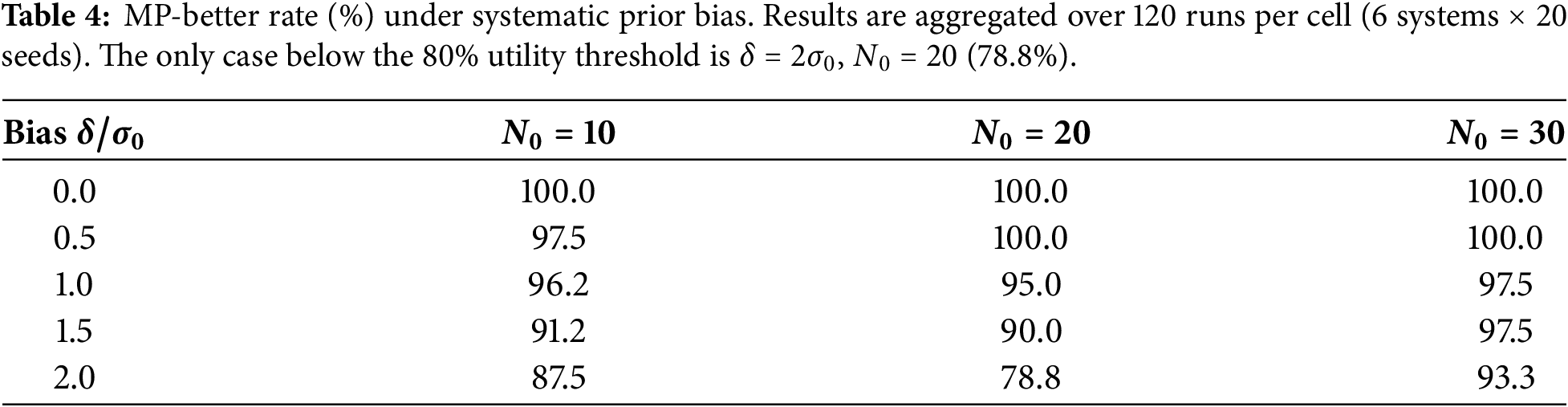
The extended grid in Fig. 6 uses 240 paired runs per cell and biases up to 4σ0. It shows a smooth degradation rather than an abrupt transition. Across N0∈{10,20,30}, MP-better rates remain above or near 80% at δ=σ0 but fall below 80% for several cells at δ≥1.5σ0. Accordingly, the revised operating guidance is conservative: MP-TCGPR is most reliable when independent validation suggests the CALPHAD boundary bias is no larger than roughly one stated prior standard deviation; larger biases require wider priors, conflict diagnostics, or reverting to MLE.

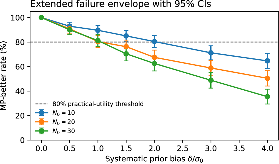
Figure 6: Extended prior-bias failure envelope with uncertainty. Error bars show approximate 95% binomial confidence intervals over 240 paired runs per cell. The dashed line denotes the 80% practical-utility threshold. Performance declines smoothly beyond δ/σ0=1; therefore the earlier 2σ0 rule is treated as a simulation-dependent observation, not as a universal safety guarantee.

5.5 Sensitivity and Higher-Dimensional Check

Table 5 reports the original prior-width sweep, and Table 6 adds the requested Ncross sensitivity. Changing Ncross from 50 to 400 leaves the N0=30 HD unchanged at 0.0074±0.0069 in the diagnostic simulation, indicating that the default Ncross=100 is not a finely tuned value for the tested budgets.

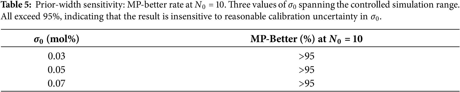
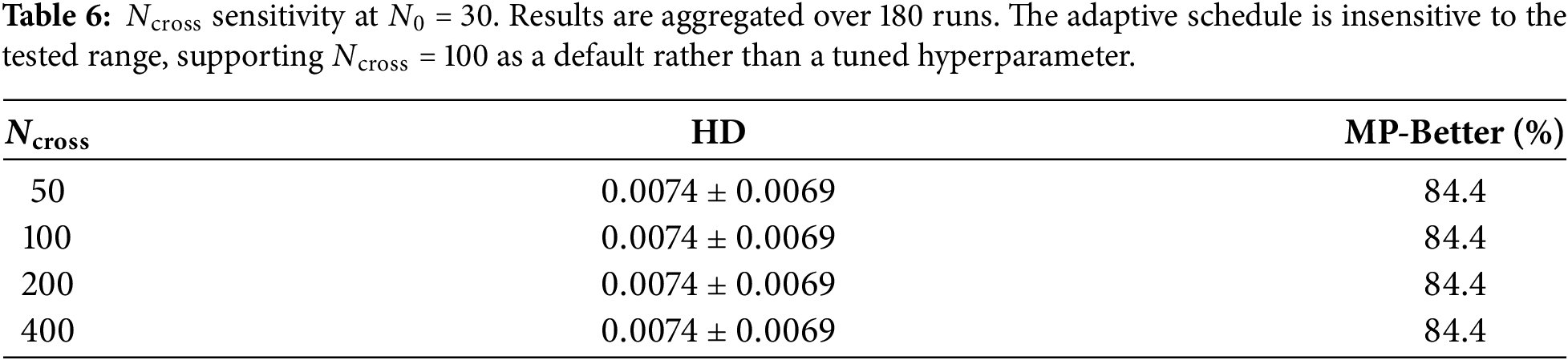
Table 7 adds a two-dimensional composition-slice experiment with a linear phase boundary. The adaptive prior reduces boundary HD from 0.1660±0.0937 to 0.0551±0.0323 at N0=20 and improves region F1 from 0.880±0.091 to 0.962±0.026. This experiment does not validate full quaternary active alloy design, but it shows that the MAP-prior idea is not intrinsically limited to one-dimensional thresholds when the boundary can be parameterized in a low-dimensional form.

5.6 Active-Learning Utility

The revised active-learning diagnostic reports both cumulative regret and best-found optimality gap over 40 runs per budget. It is a budget-level utility check rather than a full closed-loop acquisition benchmark; therefore it is used only to test whether the partition gains plausibly translate into downstream optimization gains. At a budget of 100 evaluations, adaptive MAP reduces mean cumulative regret from 0.0404 for MLE partitioning to 0.0292, while the best-found gap changes only from 0.0275 to 0.0258. These effects are directionally favorable but modest compared with the boundary HD improvement. We therefore frame the method primarily as a cold-start partition estimator; the claim that improved partitions reliably produce large downstream AL gains requires larger real-material studies.

6  Discussion

The main finding is that thermodynamic priors substantially improve cold-start composition-space partitioning. MP-TCGPR reduces normalized HD by 3.64× at N0=10, with fixed-width and CALPHAD-only baselines confirming that the gain mainly arises from a reliable boundary prior, while adaptive scheduling provides finite-sample prior attenuation. MAP analysis shows that fixed-width priors do not introduce persistent bias in regular threshold problems, as likelihood contributions dominate asymptotically. However, practical TCGPR trees involve dynamic splits and non-convex structures, requiring empirical validation beyond local theory. Prior-bias experiments reveal that MP-TCGPR is most effective when the prior center is close to the true boundary (within approximately one prior standard deviation). Larger biases can outweigh variance reduction, highlighting the need for uncertainty-aware thermodynamic priors. Active-learning results show modest downstream benefits, indicating that MP-TCGPR primarily improves cold-start partition reliability rather than serving as a complete alloy-design optimization framework.

Several limitations remain. First, the CALPHAD priors are simulated rather than queried from Thermo-Calc, PANDAT, or another production database; real database errors may be systematic, non-Gaussian, and composition- or temperature-dependent. Second, most experiments use one-dimensional cross-sections, although the new 2D slice shows that the MAP-prior idea can extend to a simple low-dimensional boundary parameterization. Third, the synthetic piecewise-GP generator is favorable to tree partitioning, so comparisons with linear models, SVM/RBF classifiers, convex-hull boundary methods, phase-field models, high-throughput screening workflows, and other Bayesian optimization or partitioning approaches remain necessary for a complete benchmark [33–35]. Extrapolation benchmarks and high-throughput materials platforms provide complementary evaluation settings [36–38]; broader materials-informatics perspectives also motivate such benchmarking [39]. Fourth, the computational cost remains small for axis-aligned thresholds (one quadratic penalty per candidate threshold), but richer 2D/3D boundary families would require more expensive optimization and stronger regularization.

Recent adjacent materials-informatics studies further illustrate the broader context in which such partition and prior-calibration problems arise, including ML-assisted aluminum-alloy design, quasi-phase prediction, interpolation–extrapolation trade-offs, polymer-material property prediction, high-throughput first-principles screening, and interface calculations [25–27]. Interpolation–extrapolation, polymer-material, high-throughput screening, and interface studies provide additional related examples [40]; first-principles interface calculations further illustrate this broader context. Overall, MP-TCGPR should be viewed as a lightweight mechanism for incorporating external thermodynamic boundary estimates into TCGPR when the uncertainty of those estimates is credible. It is most useful in the data-scarce regime and most risky when the thermodynamic prior is overconfident or biased. The revised experiments are intended to make these tradeoffs explicit rather than to overstate validation on real CALPHAD or DFT data.

7  Conclusions

This study presents MP-TCGPR, a lightweight MAP-prior extension of TCGPR that stabilizes cold-start composition-space partitioning when a thermodynamic boundary estimate is available. Theoretical analysis further shows that fixed-width MAP priors become asymptotically negligible under regularity conditions, while adaptive prior scheduling primarily serves as a finite-sample mechanism to accelerate prior release as node-level data accumulate. Controlled one-dimensional benchmarks demonstrate that MP-TCGPR achieves the largest improvement under limited initial budgets, and the CALPHAD-only and fixed-width MAP baselines further confirm that the gain mainly originates from incorporating a calibrated thermodynamic prior.

Additional diagnostics characterize the applicability and limitations of the proposed approach. Prior-bias experiments indicate that the method remains reliable when the prior center is reasonably close to the true boundary, typically within one prior standard deviation. Two-dimensional experiments further suggest that the MAP-prior formulation can extend beyond one-dimensional thresholds, although more complex boundary representations require additional investigation. The active-learning utility study shows consistent but moderate regret reduction, suggesting that the current contribution primarily lies in improving cold-start partition estimation rather than fully optimizing end-to-end alloy-design workflows.

Future studies will focus on three aspects: validating prior assumptions using production CALPHAD databases (e.g., Thermo-Calc and PANDAT) with realistic uncertainty sources, developing higher-dimensional boundary models with conflict-aware prior control, and integrating improved partitioning into complete closed-loop alloy-design campaigns with comprehensive evaluation of acquisition efficiency, GP calibration, optimization performance, and robustness under uncertain thermodynamic knowledge.

Acknowledgement: Not applicable.

Funding Statement: The authors received no specific funding for this study.

Author Contributions: Conceptualization, Haipeng Hu and Dahai Xia; methodology, Haipeng Hu and Xinjie Yao; software, Haipeng Hu and Junjie Zhu; validation, Junjie Zhu, Tao Hong and Zhoupeng Guo; formal analysis, Haipeng Hu and Xinjie Yao; investigation, Haipeng Hu, Junjie Zhu and Tao Hong; writing—original draft preparation, Haipeng Hu; writing—review and editing, Tao Hong and Junjie Zhu; visualization, Haipeng Hu and Tao Hong; supervision, Xinjie Yao, Zhoupeng Guo and Dahai Xia; project administration, Dahai Xia. All authors reviewed and approved the final version of the manuscript.

Availability of Data and Materials: Data and Material will be made available on reasonable request.

Ethics Approval: Not applicable.

Conflicts of Interest: The authors declare no conflicts of interest.

Abbreviations

The following abbreviations are used in this manuscript:

References

1. Lookman T, Balachandran PV, Xue D, Yuan R. Active learning in materials science with emphasis on adaptive sampling using uncertainties for targeted design. npj Comp Mater. 2019;5(1):21. doi:10.1038/s41524-019-0153-8. [Google Scholar] [CrossRef]

2. Balachandran PV, Xue D, Theiler J, Hogden J, Lookman T. Adaptive strategies for materials design using uncertainties. Sci Rep. 2016;6(1):19660. doi:10.1038/srep19660. [Google Scholar] [CrossRef]

3. Zhang Y, Apley DW, Chen W. Bayesian optimization for materials design with mixed quantitative and qualitative variables. Sci Rep. 2020;10(1):4924. doi:10.1038/s41598-020-60652-9. [Google Scholar] [CrossRef]

4. Tran K, Neiswanger W, Yoon J, Zhang Q, Xing E, Ulissi ZW. Methods for comparing uncertainty quantifications for material property predictions. Mach Learn Sci Technol. 2020;1(2):025006. doi:10.1088/2632-2153/ab7e1a. [Google Scholar] [CrossRef]

5. Khatamsaz D, Arroyave R, Allaire DL. Asynchronous multi-information source Bayesian optimization. J Mech Des. 2024;146(10):101708. doi:10.1115/1.4065064. [Google Scholar] [CrossRef]

6. Zong B, Li J, Yuan T, Wang J, Yuan R. Recent progress on machine learning with limited materials data: using tools from data science and domain knowledge. J Mater. 2025;11(3):100916. [Google Scholar]

7. Greenhill S, Rana S, Gupta S, Vellanki P, Venkatesh S. Bayesian optimization for adaptive experimental design: a review. IEEE Access. 2020;8:13937–48. doi:10.1109/access.2020.2966228. [Google Scholar] [CrossRef]

8. Chipman HA, George EI, McCulloch RE. Bayesian CART model search. J Am Stat Assoc. 1998;93(443):935–48. doi:10.1080/01621459.1998.10473750. [Google Scholar] [CrossRef]

9. Gramacy RB, Lee HKH. Bayesian treed Gaussian process models with an application to computer modeling. J Am Stat Assoc. 2008;103(483):1119–30. doi:10.1198/016214508000000689. [Google Scholar] [CrossRef]

10. Wei J, Chu X, Sun XY, Xu K, Deng HX, Chen J, et al. Machine learning in materials science. InfoMat. 2019;1(3):338–58. doi:10.1002/inf2.12028. [Google Scholar] [CrossRef]

11. Hart GLW, Mueller T, Toher C, Curtarolo S. Machine learning for alloys. Nat Rev Mater. 2021;6(8):730–55. doi:10.1038/s41578-021-00340-w. [Google Scholar] [CrossRef]

12. Raccuglia P, Elbert KC, Adler PDF, Falk C, Wenny MB, Mollo A, et al. Machine-learning-assisted materials discovery using failed experiments. Nature. 2016;533:73–6. doi:10.1038/nature17439. [Google Scholar] [CrossRef]

13. Lukas HL, Fries SG, Sundman B. Computational thermodynamics: the CALPHAD method. Cambridge, UK: Cambridge University Press; 2007. [Google Scholar]

14. Dinsdale AT. SGTE data for pure elements. Calphad. 1991;15(4):317–425. [Google Scholar]

15. Bocklund B, Otis R, Egorov A, Obaied A, Roslyakova I, Liu ZK. ESPEI for efficient thermodynamic database development, modification, and uncertainty quantification: application to Cu–Mg—CORRIGENDUM. MRS Commun. 2020;10(4):702–2. [Google Scholar]

16. Shahmir H, Forghani F. High-throughput computational and machine-learning design of high-entropy alloys based on thermodynamic and empirical parameters: Al-Si-Cr-Fe-(Ni,Mn) systems. Intermetallics. 2026;195(5):109328. doi:10.1016/j.intermet.2026.109328. [Google Scholar] [CrossRef]

17. Ury N, Otis R, Ravi V. Generalized method of sensitivity analysis for uncertainty quantification in CALPHAD calculations. Calphad. 2022;79:102504. doi:10.1016/j.calphad.2022.102504. [Google Scholar] [CrossRef]

18. Rasmussen CE, Williams CKI. Gaussian processes for machine learning. Cambridge, MA, USA: MIT Press; 2006. [Google Scholar]

19. Chang YA, Chen S, Zhang F, Yan X, Xie F, Schmid-Fetzer R, et al. Phase diagram calculation: past, present and future. Prog Mater Sci. 2004;49(3–4):313–45. doi:10.1016/s0079-6425(03)00025-2. [Google Scholar] [CrossRef]

20. Li S, Liu D, Li S, Chen M. A materials discovery method considering the trade-off phenomenon in machine learning prediction capabilities between interpolation and extrapolation: case study on multi-objective Mg-Zn-Al alloy design. Comput Mater Contin. 2026;87(2):14. doi:10.32604/cmc.2026.075830. [Google Scholar] [CrossRef]

21. Kaur M, Randhawa P, Jaiswal J, Dubal D, Bulakhe RN, Balakrishnan D, et al. Data-driven materials science using machine learning and computational modeling. Comput Mater Contin. 2026;88(2):4. doi:10.32604/cmc.2026.079503. [Google Scholar] [CrossRef]

22. Chen SL, Daniel S, Zhang F, Chang YA, Yan XY, Xie FY, et al. The PANDAT software package and its applications. Calphad. 2002;26(2):175–88. doi:10.1016/s0364-5916(02)00034-2. [Google Scholar] [CrossRef]

23. Otis R. Uncertainty reduction and quantification in computational thermodynamics. Comput Mater Sci. 2022;212:111590. doi:10.1016/j.commatsci.2022.111590. [Google Scholar] [CrossRef]

24. Liu F, Xiao X, Huang L, Tan L, Liu Y. Design of NiCoCrAl eutectic high entropy alloys by combining machine learning with CALPHAD method. Mater Today Commun. 2022;30:103172. doi:10.1016/j.mtcomm.2022.103172. [Google Scholar] [CrossRef]

25. Wang H, Duan Z, Guo Q, Zhang Y, Zhao Y. Machine learning design of aluminum-lithium alloys with high strength. Comput Mater Contin. 2023;77(2):1393–409. doi:10.32604/cmc.2023.045871. [Google Scholar] [CrossRef]

26. Lin Z, Yang C. Artificial intelligence design of sustainable aluminum alloys: a review. Comput Mater Contin. 2025;86(2):1–33. doi:10.32604/cmc.2025.070735. [Google Scholar] [CrossRef]

27. Zhu C, Zhao B, Naranjo Villota JL, Gao Z, Feng L. Quasi-phase equilibrium prediction of multi-element alloys based on machine learning and deep learning. Comput Mater Contin. 2023;76(1):49–64. doi:10.32604/cmc.2023.036729. [Google Scholar] [CrossRef]

28. Chen LQ. Phase-field models for microstructure evolution. Annu Rev Mater Res. 2002;32(1):113–40. doi:10.1146/annurev.matsci.32.112001.132041. [Google Scholar] [CrossRef]

29. Berger JO, Moreno E, Pericchi LR, Bayarri MJ, Bernardo JM, Cano JA, et al. An overview of robust Bayesian analysis. Test. 1994;3(1):5–124. doi:10.1007/bf02562676. [Google Scholar] [CrossRef]

30. Grunwald P, van Ommen T. Inconsistency of Bayesian inference for misspecified linear models, and a proposal for repairing it. Bayesian Anal. 2017;12(4):1069–103. [Google Scholar]

31. Harris CR, Millman KJ, van der Walt SJ, Gommers R, Virtanen P, Cournapeau D, et al. Array programming with NumPy. Nature. 2020;585:357–62. [Google Scholar]

32. Pedregosa F, Varoquaux G, Gramfort A, Michel V, Thirion B, Grisel O, et al. Scikit-learn: machine learning in Python. J Mach Learn Res. 2011;12:2825–30. [Google Scholar]

33. Shahriari B, Swersky K, Wang Z, Adams RP, de Freitas N. Taking the human out of the loop: a review of Bayesian optimization. Proc IEEE. 2016;104(1):148–75. doi:10.1109/jproc.2015.2494218. [Google Scholar] [CrossRef]

34. Frazier PI. A tutorial on Bayesian optimization. arXiv:1807.02811. 2018. [Google Scholar]

35. Dunn A, Wang Q, Ganose A, Dopp D, Jain A. Benchmarking materials property prediction methods: the Matbench test set and Automatminer reference algorithm. npj Comput Mater. 2020;6:138.Erratum in: npj Comput Mater. 2020;6:159. [Google Scholar]

36. Meredig B, Antono E, Church C, Hutchinson M, Ling J, Paradiso S, et al. Can machine learning identify the next high-temperature superconductor? Examining extrapolation performance for materials discovery. Mol Syst Des Eng. 2018;3(5):819–25. [Google Scholar]

37. Curtarolo S, Hart GLW, Nardelli MB, Mingo N, Sanvito S, Levy O. The high-throughput highway to computational materials design. Nat Mater. 2013;12(3):191–201. doi:10.1038/nmat3568. [Google Scholar] [CrossRef]

38. Jain A, Ong SP, Hautier G, Chen W, Richards WD, Dacek S, et al. Commentary: the materials project: a materials genome approach to accelerating materials innovation. APL Mater. 2013;1:011002. [Google Scholar]

39. Agrawal A, Choudhary A. Perspective: materials informatics and big data: realization of the fourth paradigm of science in materials science. APL Mater. 2016;4(5):053208. [Google Scholar]

40. Mo W, Lu Q, Zheng X, Yang M, Zeng Y, Li K, et al. CALPHAD-based cross-system knowledge transfer for rapid discovery of high-performance Al-Mg–Zn alloys. npj Comp Mater. 2026;12(1):201. doi:10.1038/s41524-026-02073-2. [Google Scholar] [CrossRef]