Cross-View Geo-Localization via Dynamic Multi-Positive Mining from Unlabeled Data

1  Introduction

Cross-view geo-localization (CVGL) aims to estimate the geographic position of a street-level image by retrieving its matching GPS-tagged satellite tile. It offers an image-based alternative when satellite navigation is weak or unavailable, and supports applications such as autonomous driving, augmented reality, and visual positioning in GPS-denied areas [1–3].

Recent supervised CVGL methods learn a shared feature space from paired ground–satellite images. Early convolutional models [4] focus on view-invariant features. Later methods reduce the cross-view gap with spatial attention, view transformation, transformer-based matching, and geometry-aware representations, including SAFA [5], L2LTR [6], TransGeo [7], GeoDTR [8], and GeoDTR+ [9]. These methods achieve strong accuracy when many paired labels are available. However, collecting such labels requires accurate GPS annotations and careful image pairing, which is expensive at city scale. Moreover, models trained in one region may degrade when the test distribution changes, as observed in GeoDTR+ [9]. Therefore, reducing the dependence on paired labels is important for practical CVGL.

Most label-efficient studies so far concentrate on the UAV-to-satellite setting, where drone and satellite images share near-vertical viewpoints and are easier to align. Pseudo pairs can be mined by clustering and cross-view cluster matching [10–12]. Ground-to-satellite localization is more challenging because a horizontal panorama and a top-down tile have little appearance overlap, causing unsupervised alignment to fail at the beginning of training. To address this, Li et al. [13] introduced a semi-supervised pipeline that first warms up the model with a small labeled subset and then mines pseudo labels from unlabeled data via mutual matching and similarity-gap filtering. Each accepted query is assigned only one reference for single-positive contrastive training, as shown in Fig. 1a.

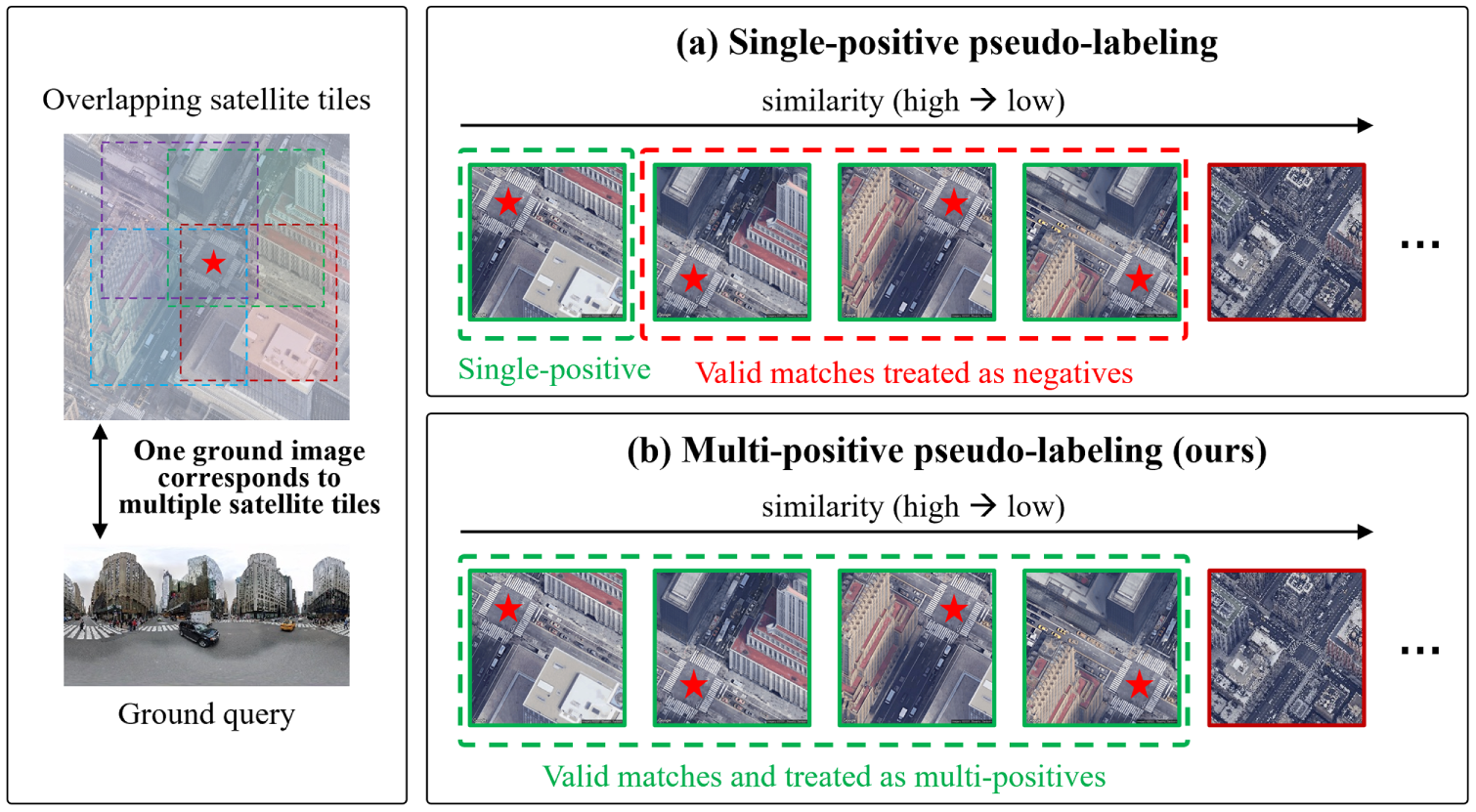
Figure 1: Single-positive pseudo-labeling (a) vs. the proposed dynamic multi-positive paradigm (b) for semi-supervised ground-to-satellite geo-localization.

Although this semi-supervised pipeline is effective, its pseudo-label selection still assumes that each query has only one positive reference. It expects the correct reference to rank clearly above all others and treats the remaining candidates as negatives. This assumption often fails in real galleries. Satellite tiles are usually sampled with overlap, and a ground image may not be located at the center of a tile. Therefore, several adjacent tiles can all be valid matches. VIGOR [14] explicitly models this many-to-many relation between ground images and satellite tiles. In this case, single-positive pseudo-labeling may reject a query when several true matches have similar scores. It may also keep only one valid tile and push the other valid tiles into the negative set. This reduces pseudo-label recall and introduces false negatives during training.

To address this limitation, we propose DMP-Geo, a semi-supervised cross-view geo-localization method that mines multiple positives for each query from unlabeled data, as illustrated in Fig. 1b. DMP-Geo first employs a Bird’s-Eye Fusion Encoder (BFE) to combine the original panorama with its bird’s-eye-view (BEV) projection, which provides the query representation with additional top-down geometric cues. Based on this representation, Adaptive Multi-Positive Mining (AMM) analyzes the ranked similarity sequence, identifies the first clear score drop, and retains the candidates before this boundary as provisional positives. These candidates are then verified by mutual consistency to reduce false matches. In this way, the number of pseudo positives is determined adaptively for each query instead of being fixed to one. Finally, a confidence-weighted multi-positive contrastive loss assigns larger weights to more reliable positives and optimizes the model with all verified positives.

Our main contributions are summarized as follows.

•   We propose DMP-Geo, a semi-supervised cross-view geo-localization method that dynamically adapts the number of pseudo positives for each query and reduces false-negative supervision in many-to-many galleries.

•   We design a bird’s-eye fusion encoder (BFE) that integrates the original panorama with its bird’s-eye-view projection, producing a query representation that is more consistent with satellite imagery and thus alleviating the cross-view appearance gap.

•   We introduce AMM, an adaptive breakpoint-based mining strategy with mutual consistency verification. AMM mines multiple reliable pseudo positives from unlabeled data and improves pseudo-label recall while maintaining high precision.

•   Experiments on CVUSA, CVACT, and VIGOR show that DMP-Geo consistently outperforms the existing semi-supervised baseline under 10%–30% annotation budgets. On VIGOR, it achieves the strongest Cross-area R@1 among the compared methods, demonstrating strong generalization to unseen cities.

2  Related Work

2.1 Supervised Cross-View Geo-Localization

Cross-view geo-localization has been extensively studied in both ground-to-satellite and UAV-to-satellite retrieval. Closely related to this retrieval-based localization paradigm, visual place recognition also aims to identify the place depicted by a query image from a geo-referenced database, and recent methods have improved retrieval robustness under domain or environmental changes [15,16]. Early ground-to-satellite studies introduced deep convolutional networks to learn viewpoint-invariant representations from paired ground panoramas and aerial images [4]. Subsequent methods further reduce the cross-view discrepancy by designing view transformation, attention, and local feature aggregation mechanisms. For example, SAFA [5] uses polar transformation and spatial-aware feature aggregation. L2LTR [6] introduces Transformer-based layer-to-layer matching, and TransGeo [7] suppresses irrelevant regions with attention-guided non-uniform cropping. GeoDTR and GeoDTR+ [8,9] further learn geometric correspondence through disentangled and generic alignment strategies. Recent methods such as FRGeo [17] and VimGeo [18] improve geometric-spatial alignment and efficient cross-view modeling.

UAV-to-satellite geo-localization has also been actively explored after the construction of University-1652 [19]. Related UAV visual localization studies have also investigated multi-modal scene matching, where visible, infrared, and satellite images are matched by combining target recognition, deep feature matching, and mismatch filtering [20]. Representative methods such as LPN [21], PCL [22], and MCCG [23] improve local feature extraction and multi-view fusion under the aerial-to-aerial retrieval setting. Despite their effectiveness, the above supervised approaches depend on abundant paired annotations. This dependence makes data collection expensive and limits practical deployment in new cities or domains where only a small portion of labeled pairs is available.

2.2 Label-Efficient Cross-View Geo-Localization

To reduce annotation cost, recent studies have investigated unsupervised or semi-supervised CVGL. Most unsupervised efforts focus on UAV-to-satellite retrieval. Because UAV and satellite images share approximately top-down viewpoints, their feature distributions are more compatible than those of ground panoramas and satellite tiles. Under this relatively aligned setting, methods such as EM-CVGL [11], paired-labeled-data-free learning [10], unsupervised multi-view UAV localization [12], and coarse-to-fine cluster matching [24] mine pseudo pairs by clustering or mutual matching in the embedding space. Xie et al. [25] further introduce the UAV view as an intermediate bridge to assist cross-view graph learning.

However, these unsupervised UAV-oriented paradigms cannot be directly transferred to ground-to-satellite geo-localization. A ground panorama is captured from a horizontal perspective, whereas the satellite image is observed from a top-down perspective. The resulting projection discrepancy is much larger than that in UAV-to-satellite matching, making direct cross-view clustering unreliable at the beginning of training. Ground-to-satellite localization therefore usually requires a small amount of annotated data for warm-up before unlabeled data can be safely exploited. Li et al. [13] are the first to explore this semi-supervised setting, generating high-confidence pseudo labels through mutual matching and similarity-gap filtering, but their pseudo-label selection still follows a one-to-one assumption that treats every reference other than the single chosen one as negative. This assumption is at odds with the many-to-many correspondences that arise in real galleries such as VIGOR [14], where adjacent tiles jointly cover a single location. Our work keeps the warm-up stage required by this setting, but replaces the single-positive pseudo label with a variable-size positive set for each query, as described in Section 3.

2.3 Multi-Positive and Neighbor-Based Contrastive Learning

Multi-positive contrastive and metric learning methods generally optimize positive relations supplied by class labels, augmented views, temporal co-occurrence, labeled pairs, or predefined neighbor-selection rules. Supervised Contrastive Learning (SupCon) defines multiple positives using class labels and augmented views [26], whereas Multi-Similarity Loss mines and weights informative positive and negative pairs within labeled batches [27]. MIL-NCE aggregates a predefined bag of temporally related video–text candidates [28]. In self-supervised learning, NNCLR retrieves the nearest neighbor from a representation-space support set and treats it as an additional positive [29], while false-negative cancellation avoids repelling samples that are likely to be semantic neighbors [30].

These methods rely on positives defined by supervision, preconstructed candidate bags, or generic representation-space neighborhood rules. The setting considered in DMP-Geo is different: for an unlabeled ground query in an overlapping satellite gallery, both the identities and the number of matching tiles are unknown, and an unverified nearest-neighbor rule can be unreliable under the severe cross-view discrepancy. DMP-Geo therefore performs positive-set discovery before multi-positive optimization. It estimates a query-dependent boundary from the first pronounced drop in the ranked cross-view similarities, verifies the provisional candidates through reverse Top-1 consistency, and assigns confidence weights within the verified set. Its distinction lies in combining query-dependent positive-set discovery, mutual-consistency verification, and confidence-weighted multi-positive optimization within an alternating semi-supervised ground-to-satellite framework.

3  Method

3.1 Overview

Fig. 2 shows the overall pipeline of DMP-Geo. Let 𝒟l={(gi,sπ(i))} denote the small set of labeled ground–satellite pairs, 𝒟u={gi} the unlabeled ground queries, and 𝒮={sj}j=1Ns the satellite reference gallery. A dual-branch ground encoder and a satellite encoder map both domains into a shared d-dimensional space, in which each query is represented by a bird’s-eye fused feature that carries both fine-grained ground texture and satellite-like overhead geometry.

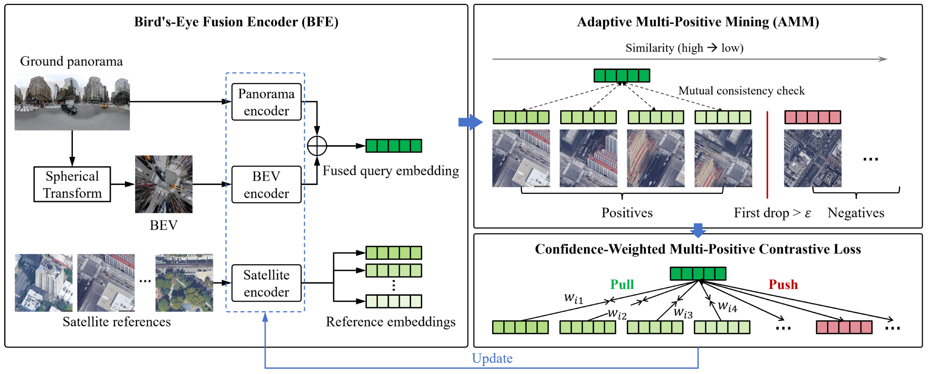
Figure 2: Pipeline of DMP-Geo. The fused query embedding and the reference embeddings are produced by the dual-branch and satellite encoders, respectively. AMM scans the ranked similarities of each unlabeled query, accepts all candidates above the first pronounced similarity drop, and verifies them via mutual consistency. The resulting multi-positive sets, together with in-batch references, drive the confidence-weighted multi-positive contrastive objective, and mining and training alternate iteratively.

Training proceeds in two phases. A short supervised warm-up on 𝒟l first moves the two encoders away from random initialization. This step is important in ground-to-satellite matching because a panorama and a satellite tile share little low-level appearance, and rankings before warm-up are usually unreliable. After warm-up, the model alternates between mining and updating once per epoch. The mining stage analyzes the current similarity ranking of every unlabeled query and assigns it an adaptive set of pseudo positives. The update stage then optimizes the encoders using batches formed by the queries, their mined positives, and the remaining in-batch references. Since pseudo labels are regenerated at the beginning of each epoch, better features can lead to more reliable mining in later epochs. Algorithm 1 summarizes the procedure.

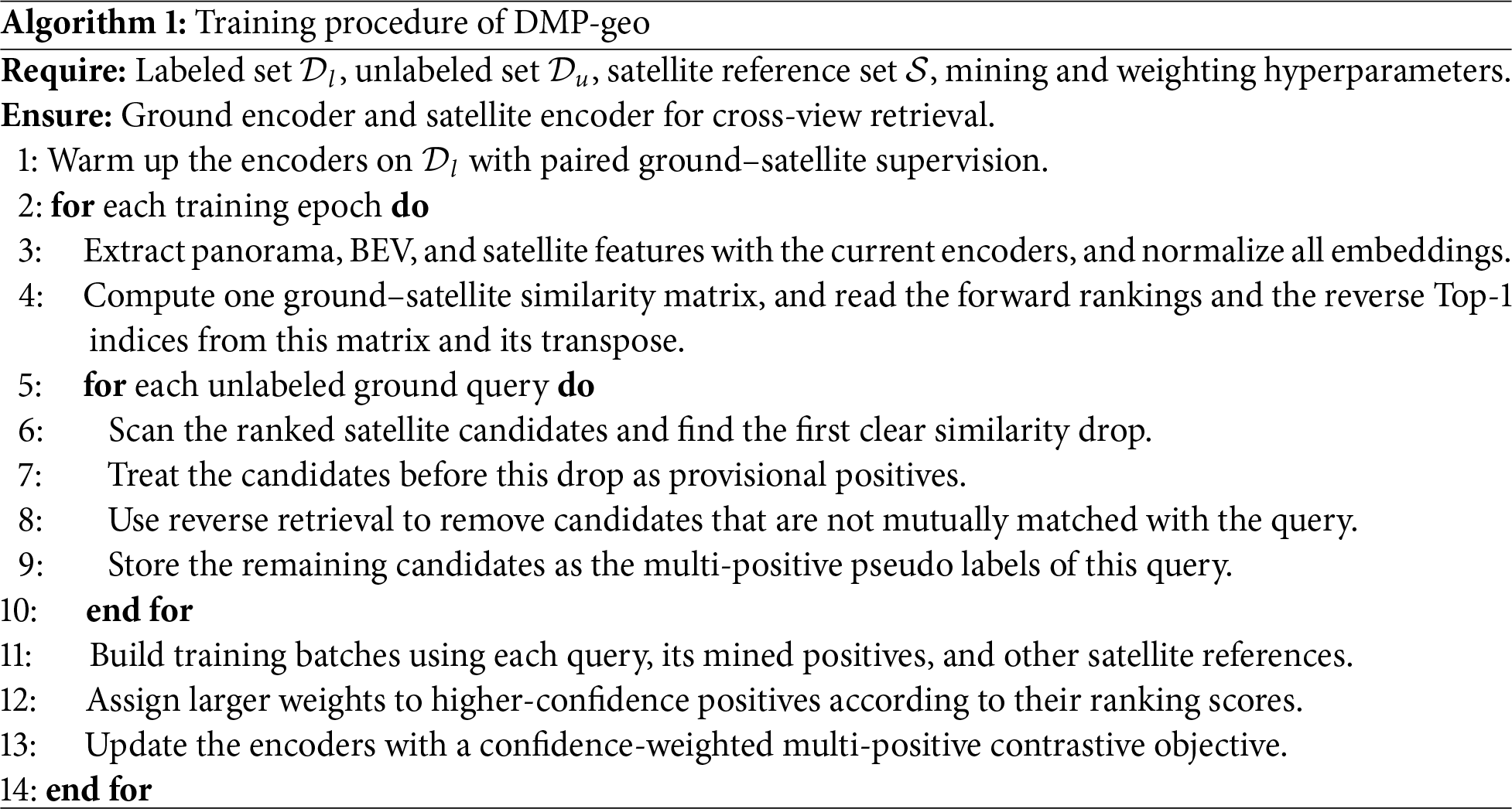
These three components address different needs of the loop. The Bird’s-Eye Fusion Encoder makes the query embedding more comparable to satellite tiles. Adaptive Multi-Positive Mining decides how many positives to keep for each query, and the confidence-weighted contrastive loss turns these variable-size positive sets into stable training signals.

3.2 Bird’s-Eye Fusion Encoder

Every pseudo positive is mined from the similarity ranking that the query embedding produces, so the query must be geometrically comparable to satellite tiles before mining can be trusted. A single panorama branch cannot meet this need, because its horizontal field of view arranges scene content in a way that has little geometric resemblance to the bird’s-eye layout of a satellite tile. As a result, the rankings used for early-stage mining are noisy. The Bird’s-Eye Fusion Encoder (BFE) reduces this geometric gap by pairing each ground image with a complementary bird’s-eye-view (BEV) description. The panorama keeps a 360∘ field of view and rich texture that is discriminative yet misaligned with the overhead view, whereas the BEV projection re-renders the scene onto a top-down plane and recovers the road layouts and building footprints that approximate the satellite domain. Fusing the two gives the query feature both texture cues and a more satellite-like layout, which helps produce more reliable rankings for mining.

BEV projection. The BEV branch relies on a spherical projection that maps the panorama onto a top-down plane through a virtual overhead camera [31]. Concretely, let the panorama have size Wp×Hp with pixel coordinates (up,vp), and let the target BEV image have size Wb×Hb with pixel coordinates (ub,vb). The focal length of the virtual camera is f=0.5Wb/tan⁡(fov), where fov is its half field-of-view angle. Each BEV pixel is then traced back to its source location in the panorama by

up=Wp2(1−atan2⁡(xb,yb)π),vp=Hp(12−atan2⁡(−f,db)π),(1)

where xb=ub−Wb/2 and yb=Hb/2−vb are the BEV pixel coordinates measured from the projection center of the virtual camera, and db=xb2+yb2 is the distance of the pixel to that center. Sampling the panorama at the coordinates given by Eq. (1) for every BEV pixel produces the BEV image, which we denote by Π(gi). The half field-of-view angles used for each dataset, together with their provenance, are reported in Section 4.1.

Feature fusion. Two parallel encoders then process the two descriptions. The encoder ϕp consumes the raw panorama gi, and ϕb consumes its BEV image Π(gi). Their outputs are merged by element-wise averaging,

qi=12(ϕp(gi)+ϕb(Π(gi))).(2)

We keep the fusion parameter-free instead of using a learnable attention module or projection head, because a heavier module may overfit the few labeled pairs during warm-up and make later mining less stable. Element-wise averaging keeps the two branches balanced, adds no parameters, and empirically yields a smoother similarity space. Section 4.4 examines this choice empirically: an inference-time branch-weight scan peaks at equal weights, a descriptor-level cross-attention variant performs substantially worse at a large parameter cost, and a learnable two-scalar gate converges to an almost symmetric split. These observations support averaging as a simple and stable choice for the evaluated model and protocol, without implying that averaging is universally preferable to attention-based fusion. Each satellite reference is encoded independently as rj=ϕr(sj).

3.3 Adaptive Multi-Positive Mining

Existing semi-supervised pseudo-labeling fixes the number of positives to one and treats every other reference as a negative. This is not suitable for many-to-many galleries, where several adjacent tiles may cover the same location. Adaptive Multi-Positive Mining (AMM) instead keeps a variable number of positive candidates for each query. The design is based on a simple observation. True tiles covering the same location are often spatially close and visually similar, so their similarities to the query tend to form a compact group at the top of the ranking. Once the ranking reaches non-matching tiles, the score usually drops. AMM uses this drop to estimate the positive boundary, and then applies a mutual consistency check to reduce false positives.

Dynamic gap detection. Given a query gi, we compute its similarity sij=⟨qi,rj⟩ to every satellite embedding and sort the references in descending order, obtaining the index sequence {j1,j2,…,jNs}. Rather than inspecting only the Rank-1/Rank-2 gap, AMM traverses the head of the sequence and locates the first adjacent pair whose similarity decrease exceeds a threshold ε,

bi=min{k|si,jk−si,jk+1>ε}.(3)

The position bi marks the transition from the positive cluster to the non-matching region, and all candidates ranked no lower than bi form the provisional positive set 𝒞i={j1,…,jbi}, whose size adapts automatically to each query. This single mechanism resolves both failure modes of one-positive mining. When several true tiles score very closely, the boundary moves rightward to include them all, so the Rank-1/Rank-2 gap is no longer a bottleneck, and when a query has only one clear match, the first large drop often appears after Rank-1, so AMM usually keeps only one positive.

Mutual consistency check. A breakpoint alone cannot remove visually confusing distractors such as repetitive road segments or near-duplicate building blocks that occasionally enter the head of the ranking. To refine the provisional set, each candidate sj∈𝒞i is used as a reverse query against all ground images and survives only when the original query gi is returned at the top of that reverse ranking,

ℳi={j∈𝒞i | gi=arg⁡maxg∈𝒟u∪𝒟l⟨q(g),rj⟩}.(4)

This check is used because a forward match only shows that sj is similar to gi. The reverse match further requires gi to be the most similar query for sj, which helps remove tiles that look generic and are similar to many queries. In implementation, the encoders are run once per mining round to form a single ground–satellite similarity matrix; the forward rankings and the reverse Top-1 indices are then read from this matrix and its transpose, so no candidate-specific feature extraction and no additional full-gallery retrieval are performed. The surviving candidates form the final multi-positive set ℳi. Compared with Rank-1/Rank-2 gap filtering, this two-stage procedure can keep more true matches through the adaptive boundary, while the reverse check keeps precision high. We quantify this trade-off in Section 4.6. Since mining is repeated every epoch, candidates rejected in early epochs may be selected later when the representation improves. Each mining round replaces the pseudo-label sets of the previous round rather than appending to a cumulative pool, so earlier mining errors are not permanently retained.

3.4 Confidence-Weighted Multi-Positive Contrastive Loss

The standard InfoNCE loss supports a single positive per anchor. If it is directly used with the sets produced by AMM, all but one mined positive may be pushed into the negative term, which brings back the false-negative problem. Treating all positives equally avoids this problem, but it ignores their different reliability. The top-ranked positive is usually more reliable, while lower-ranked positives may still contain noise even after the mutual check. Therefore, we use a loss that supports a variable number of positives and weights them according to their confidence.

Batch composition. Let ℬq and ℬr denote the query and reference indices of a training batch. For query i∈ℬq, the in-batch positives are ℳiB=ℳi∩ℬr, and all remaining batch references ℬr∖ℳiB serve as negatives.

Confidence weights. We convert the within-set similarity ordering into a soft confidence distribution via a temperature-scaled softmax over the gradient-detached scores restricted to the positive set,

ωij=exp(sg(sij)/γ)∑k∈ℳiBexp(sg(sik)/γ),j∈ℳiB,(5)

and ωij=0 otherwise. Here γ is the ranking temperature and sg(⋅) is the stop-gradient operator, so the weights act as fixed targets rather than trainable quantities and prevent a degenerate shortcut in which the model merely inflates its own confidence. Since ∑j∈ℳiBωij=1, each weight expresses the relative confidence of the corresponding pseudo positive. A small γ sharpens the distribution toward the top-ranked positive, while a large one approaches uniform treatment and recovers the unweighted multi-positive loss as a special case.

Objective. The per-query loss aggregates the weighted positives in the numerator and lets every non-positive batch reference compete in the denominator,

ℓi=−log⁡∑j∈ℳiBωijexp⁡(sij)∑j∈ℳiBωijexp⁡(sij)+∑k∈ℬr∖ℳiBexp⁡(sik),(6)

and the batch loss averages over all queries,

ℒ=1|ℬq|∑i∈ℬqℓi.(7)

The gradient of ℓi is scaled by ωij for each positive. Thus, higher-confidence positives have a larger effect, while lower-confidence positives contribute less. This reduces the impact of possible false positives. Meanwhile, the members of ℳi are excluded from the negative term, so valid matches are not pushed away as negatives. The objective can therefore handle a variable number of positives while still using in-batch negatives for discrimination.

4  Experiments

4.1 Datasets and Implementation Details

Datasets. Experiments are conducted on three mainstream cross-view geo-localization benchmarks: CVUSA [4], CVACT [32], and VIGOR [14].

CVUSA primarily comprises rural U.S. ground-satellite pairs. It provides 35,532 training pairs and 8884 validation pairs aligned in both location and orientation.

CVACT focuses on urban areas in Canberra, Australia. It contains 35,532 training pairs and 8884 validation pairs. Image pairs are also aligned. Compared to CVUSA, CVACT presents greater challenges in dense urban settings.

VIGOR collects 105,214 street-view images and 90,618 satellite images from four major U.S. city centers: New York, San Francisco, Chicago, and Seattle. Overlapping tiles, center offsets, and occlusions create genuine many-to-many correspondences, making it substantially more challenging than both CVUSA and CVACT. We follow both the official Same-area protocol and the Cross-area protocol (trained on New York and Seattle, tested on San Francisco and Chicago). The ablation and analysis experiments below use the Chicago split of the Same-area protocol, whose training set contains 12,740 ground panoramas and whose test set contains 12,739, while the city gallery holds 22,308 satellite tiles. Each panorama has one primary positive and three semi-positive neighboring tiles, all of which are regarded as valid matches. Thus, the training split contains 12,740×4=50,960 annotated positive relations. Under the 30% protocol, only the selected labeled subset is exposed during training; the remaining annotations are used only for post-hoc pseudo-label evaluation.

Implementation Details. ConvNeXt-Base [33], initialized from ImageNet-22K pre-training followed by ImageNet-1K fine-tuning, serves as the backbone of all encoders. Panoramas are resized to 512×128. BEV projections and satellite tiles are resized to 256×256. Random cropping, horizontal flipping, and color jitter are applied for augmentation. All encoders are optimized with Adam (β1=0.5, β2=0.999, weight decay 0) at an initial learning rate of 1×10−4, which is decayed per epoch by a cosine schedule without restarts, ηt=η0[1+cos⁡(πt/T)]/2. Every batch pairs 40 queries with 40 references, so |ℬq|=|ℬr|=40. Training runs for T=100 epochs on a single NVIDIA RTX A6000 (48 GB), of which the first 8 epochs form the supervised warm-up.

The spherical projection uses fields of view of 87.5∘, 85∘, and 85∘ on CVUSA, CVACT, and VIGOR, respectively. These values are half field-of-view angles in the focal-length definition of Section 3.2. The corresponding full apertures, 175∘ for CVUSA and 170∘ for CVACT, are taken from the public preprocessing scripts released by Li et al. [13], which implement the projection of Eq. (1) introduced in [31]. No corresponding script is provided for VIGOR, so we reuse the CVACT urban-scene setting of 170∘. None of the three values was selected by observing test performance.

The gap threshold ε is set to 0.05, 0.025, and 0.035 on CVUSA, CVACT, and VIGOR, respectively, and the ranking temperature is fixed at γ=0.05 throughout. These three values are not tuned on our data: they are the similarity-gap thresholds released by Li et al. [13] for the same three benchmarks. Their filter applies the threshold to the Rank-1/Rank-2 gap, whereas Eq. (3) applies it to the first adjacent gap in the ranked head; both operate on the same similarity-difference scale, so the published per-dataset values transfer directly to our criterion. We additionally verify that they are consistent with a calibration that uses only labels available during training. For every labeled query we measure the boundary gap, that is, the similarity difference between the last annotated positive in the ranked head and the first negative below it. On VIGOR Chicago the median of these gaps is 0.0328, close to the adopted 0.035; the median is used rather than the mean because the distribution is right-skewed by a few easy queries with very large separations. No validation or test retrieval score enters this choice at any point. The same values, the same γ, and the same once-per-epoch mining frequency are used for all three datasets and all annotation budgets reported below, and Section 4.5 reports a controlled sensitivity analysis of ε, γ, and the warm-up length. Unless otherwise stated, the semi-supervised protocol randomly keeps a labeled subset (10% on CVUSA/CVACT, 30% on VIGOR) for warm-up and treats the rest of the training data as unlabeled; pseudo-label mining and model updating then alternate epoch by epoch.

Evaluation Metrics. Retrieval quality is reported as Top-k recall (R@k), where a query counts as localized if any of its ground-truth tiles appears among the k nearest references under cosine similarity. R@1% uses k equal to 1% of the gallery size. Among these, R@1 is the strictest and most informative metric for our setting, since it directly reflects whether the correct tile is placed at the very top of the ranking, while R@1% is nearly saturated on the one-to-one datasets and mainly reflects coarse global feature quality.

4.2 Comparison with State-of-the-Art Methods

We compare DMP-Geo with the semi-supervised ground-to-satellite method of Li et al. [13], the most direct competitor in unlabeled-data exploitation, and against recent fully supervised models including L2LTR [6], TransGeo [7], GeoDTR [8], GeoDTR+ [9], FRGeo [17] and VimGeo [18].

The method of Li et al. [13] serves as the primary semi-supervised baseline because it follows the same ground-panorama/satellite setting and small-label warm-up protocol. The fully supervised results serve as performance references. Recent label-efficient UAV–satellite methods are not included in these tables because they use aerial or UAV images rather than ground panoramas, are evaluated on different datasets and retrieval protocols, or require an additional UAV view as a bridge. These differences change both the cross-view gap and the available supervision, making their published results not directly comparable to our two-view ground-panorama/satellite setting.

4.2.1 Results on CVUSA and CVACT

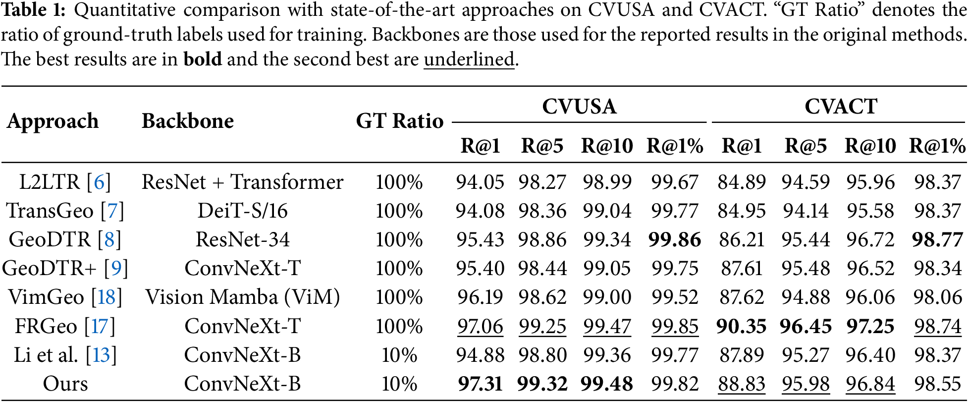
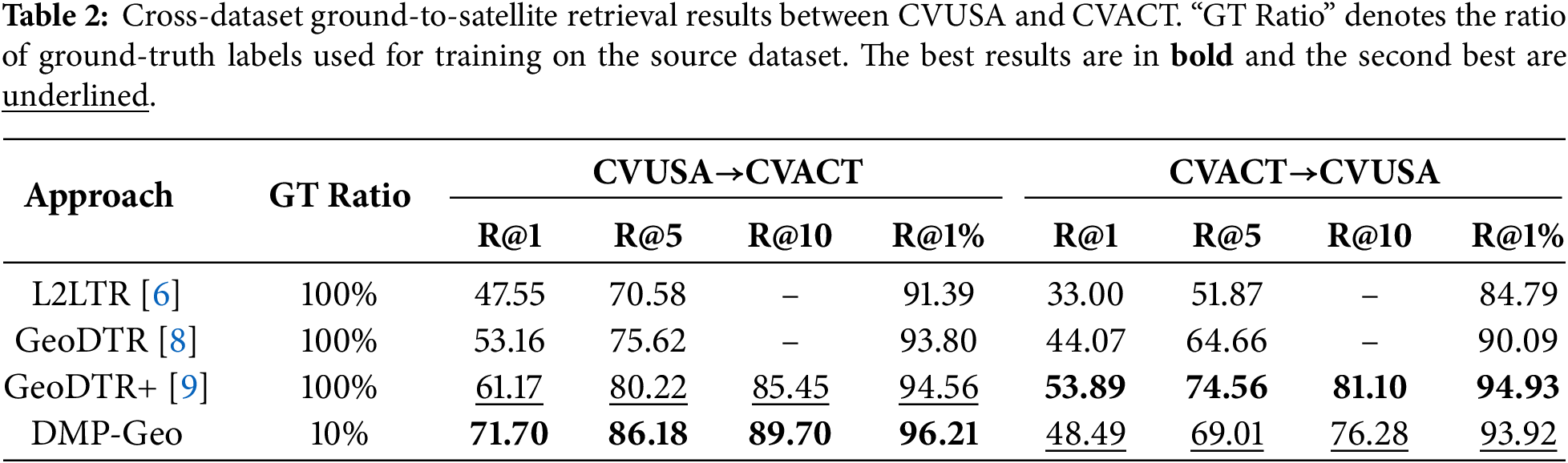
Although CVUSA and CVACT are mostly based on one-to-one pairing, near-duplicate tiles and similar neighbors still exist, so adaptive multi-positive mining remains useful. As reported in Table 1, with only 10% of the labels DMP-Geo reaches 97.31% R@1 on CVUSA and 88.83% R@1 on CVACT, exceeding the semi-supervised baseline of Li et al. by 2.43 and 0.94 percentage points, respectively. Two points are worth noting. First, this comparison controls the backbone and the initialization and therefore provides the clearest evidence for the proposed training changes. DMP-Geo is also numerically higher than several fully supervised entries, including FRGeo on CVUSA (97.06%), and higher than VimGeo (87.62%) and GeoDTR+ (87.61%) on CVACT while still trailing FRGeo there. Because these methods use different backbones, as now made explicit in Table 1, we report these differences without attributing them solely to the proposed components. Second, even on these near one-to-one datasets, the multi-positive treatment does not hurt performance. When a query has only one clear match, AMM usually keeps only one positive and behaves similarly to conventional single-positive training.

We further evaluate cross-dataset generalization between CVUSA and CVACT. The model is trained on the source dataset using 10% labeled data and the remaining source data as unlabeled data, then tested on the target dataset without any fine-tuning. This protocol is much harder than within-dataset evaluation, as the model must transfer across different geographic layouts, satellite appearances, and ground-view statistics. As shown in Table 2, with only 10% source labels DMP-Geo reaches 71.70% R@1 on CVUSA→CVACT, clearly ahead of all fully supervised competitors (e.g., 61.17% for GeoDTR+), and 48.49% on CVACT→CVUSA, surpassing L2LTR and GeoDTR though below GeoDTR+. The strong CVUSA→CVACT result supports our expectation that pseudo-label mining from relative similarity structure, combined with the geometry-aware representation learned by BFE, transfers better than the absolute region-specific cues that fully supervised models tend to overfit. The two directions are, however, clearly asymmetric, and we retain the weaker one rather than reporting only the favorable direction. One plausible explanation is that CVACT is geographically concentrated in Canberra, whereas CVUSA spans a much broader range of U.S. road layouts, building styles, vegetation, and imaging conditions, so training on the more concentrated source covers the diverse CVUSA target less completely. We present this as a plausible interpretation rather than an established cause, and the stronger GeoDTR+ result in this direction also indicates that its geometric disentanglement remains advantageous for this particular transfer setting.

4.2.2 Results on VIGOR

VIGOR is the benchmark that best reflects many-to-many correspondences and therefore directly tests the core motivation of this work. As shown in Table 3, DMP-Geo achieves 61.15% R@1 under the Same-area protocol with only 30% labeled data. This result is higher than GeoDTR+ and GeoDTR, while still remaining below TransGeo and the strongest fully supervised method FRGeo. Concretely, it is 0.33 and 10.11 percentage points below TransGeo and FRGeo, respectively. The remaining gap under Same-area is expected because fully supervised methods can access complete labeled correspondences, whereas DMP-Geo uses only a limited labeled subset and relies on mined pseudo positives.

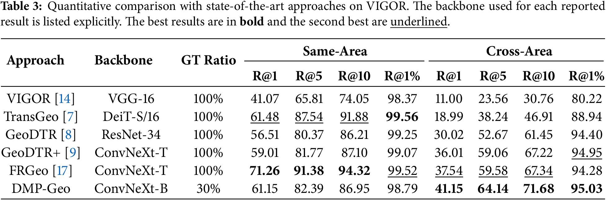
The Cross-area setting gives a clearer view of generalization across regions. Under this protocol, DMP-Geo reaches 41.15% R@1, outperforming all compared fully supervised methods. It exceeds FRGeo by 3.61 percentage points and GeoDTR+ by 5.14 percentage points. Its Same-area to Cross-area R@1 drop is 20.00 points, smaller than those of VIGOR, TransGeo, GeoDTR, GeoDTR+, and FRGeo. These results suggest that learning from adaptive multi-positive pseudo labels and bird’s-eye fused representations reduces the dependence on region-specific cues and improves robustness when the test cities change. Since Cross-area trains only on New York and Seattle and evaluates on the completely unseen cities of San Francisco and Chicago, this specifically supports transfer to unseen cities; it does not remove the Same-area gap noted above. Together with the bidirectional CVUSA/CVACT transfer, it provides two complementary forms of cross-domain evidence. All three benchmarks nevertheless rely on established acquisition pipelines and do not cover the full range of weather, season, sensor, and country-scale shifts encountered in deployment, which we leave to future work.

4.3 Ablation Study

Component contributions are examined on VIGOR (Chicago) under annotation budgets from 5% to 30%, starting from the panorama-only single-positive baseline of Li et al. [13] and adding BFE and AMM (the latter trained with the confidence-weighted multi-positive loss). Table 4 supports three observations.

First, both components are beneficial at every budget, and their value peaks under the weakest supervision. At 5% labels, BFE and AMM contribute +5.54 and +11.07 R@1 respectively, lifting the baseline from 25.82% to 42.43%, a total of +16.61 points. This confirms that the proposed designs convert unlabeled data into useful supervision when labels are scarce, which is the most important setting for a label-efficient method.

Second, the two components play distinct and complementary roles. BFE acts on the representation and therefore gives a fairly stable additive gain across budgets (+5.54, +9.81, +2.60, and +2.07 R@1 from 5% to 30%), being most pronounced when the warm-up signal is weakest and a geometry-aligned embedding is hardest to learn from labels alone. AMM acts on the supervision and is most effective when pseudo-label recall is the bottleneck. Its increment is largest at 5% (+11.07 R@1) and decreases as more labels make the head of the ranking cleaner on its own (+0.29, +0.26, and +0.53 at 10%–30%). The contrast indicates that under extreme label shortage the limiting factor is how many reliable positives can be recovered, which is exactly what the adaptive multi-positive boundary addresses.

Third, the two components remain complementary as the label budget grows. With 30% annotations the full model reaches 63.02% R@1, recovering 92.1% of the 68.40% R@1 attained by a fully labeled baseline at less than one third of the annotation cost. Overall, the ablation shows that stabilizing the representation (BFE) and enriching the supervision (AMM with the multi-positive loss) are both necessary, and that their combination, not either alone, is what closes most of the gap to full supervision.

4.4 Multi-Positive Objective and Feature-Fusion Analysis

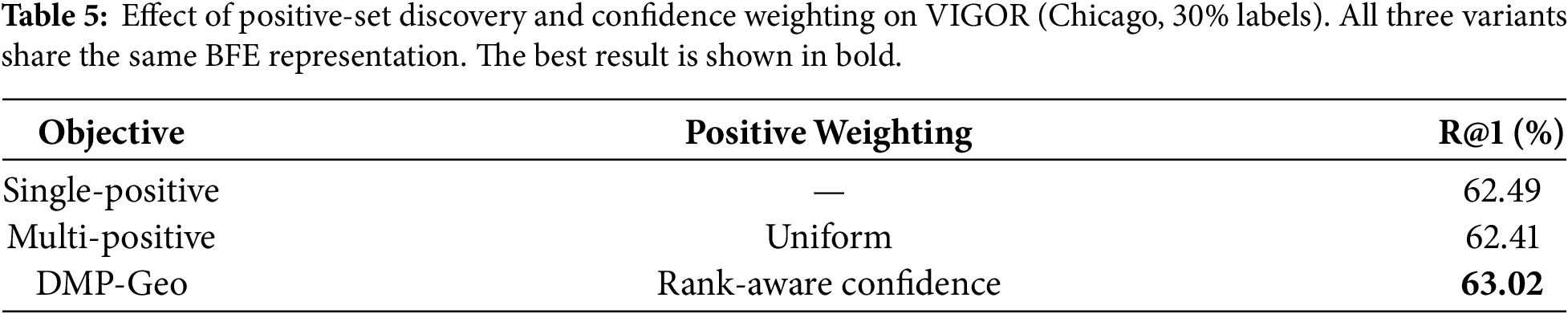
Effect of confidence weighting. To determine whether discovering multiple positives is sufficient by itself, we compare three variants that share the same BFE representation and differ only in the training objective. The single-positive variant corresponds to the “+BFE” row of Table 4 and reaches 62.49% R@1. Replacing its single pseudo positive by the AMM-mined positive set, with the confidence weights of Eq. (5) replaced by a uniform distribution over the members of that set and all other settings unchanged, reaches 62.41%. Restoring the rank-aware confidence weights reaches 63.02%. As shown in Table 5, uniform multi-positive training therefore does not improve over the single-positive variant, whereas rank-aware weighting improves R@1 by 0.61 percentage points over uniform weighting and by 0.53 percentage points over single-positive training. Positive-set discovery and confidence-aware weighting are thus complementary rather than independently sufficient: retaining several pseudo positives helps only when their unequal reliability is taken into account. Since uniform weighting is the limiting case of a large ranking temperature, this comparison also bounds the effect of γ at one end of its range.

Fixed branch-weight analysis. We next analyze the relative contribution of the two branches using the trained model that attains 63.02% R@1. At inference time the fused descriptor is replaced by q=wqBEV+(1−w)qpano without retraining, and w is scanned from 0 to 1. This post-hoc experiment diagnoses branch complementarity within a single model rather than replacing a train-time fusion ablation. Table 6 shows a clear peak at w=0.5, and moving toward either single branch reduces R@1 substantially, which indicates that the panorama and BEV descriptors carry complementary information.

Adaptive fusion variants. We further evaluate two learnable alternatives to averaging. The first is a descriptor-level cross-attention variant in which the BEV descriptor forms the query and both descriptors form the keys and values. Because the fused descriptors are d=8192-dimensional, its four d×d query, key, value and output projections add roughly 268M parameters, making it far heavier than the parameter-free mean; it reaches only 50.51% R@1, that is, 12.51 points lower. This suggests that the additional capacity is difficult to optimize with a small labeled warm-up set, rather than that attention-based fusion is inherently unsuitable. The second is a train-time two-scalar gate initialized at 0.5/0.5, which converges to BEV/panorama weights of 0.495/0.505, indicating that the optimization does not develop a stable asymmetric preference for either branch. Together with the fixed-weight curve, these results support element-wise averaging as a simple and stable choice under the evaluated limited-label protocol, although they do not establish that averaging is superior to every possible lightweight attention design.

4.5 Hyperparameter Sensitivity

Mining and weighting introduce three explicit hyperparameters: the gap threshold ε, the ranking temperature γ, and the length of the supervised warm-up. We therefore report a controlled sensitivity analysis on VIGOR (Chicago, 30% labels). For the ε and γ experiments, all runs start from the same epoch-8 warm-up checkpoint. For warm-up sensitivity, the supervised stage is run for 4, 8, or 12 epochs, while all remaining settings are kept unchanged. The results are summarized in Table 7.

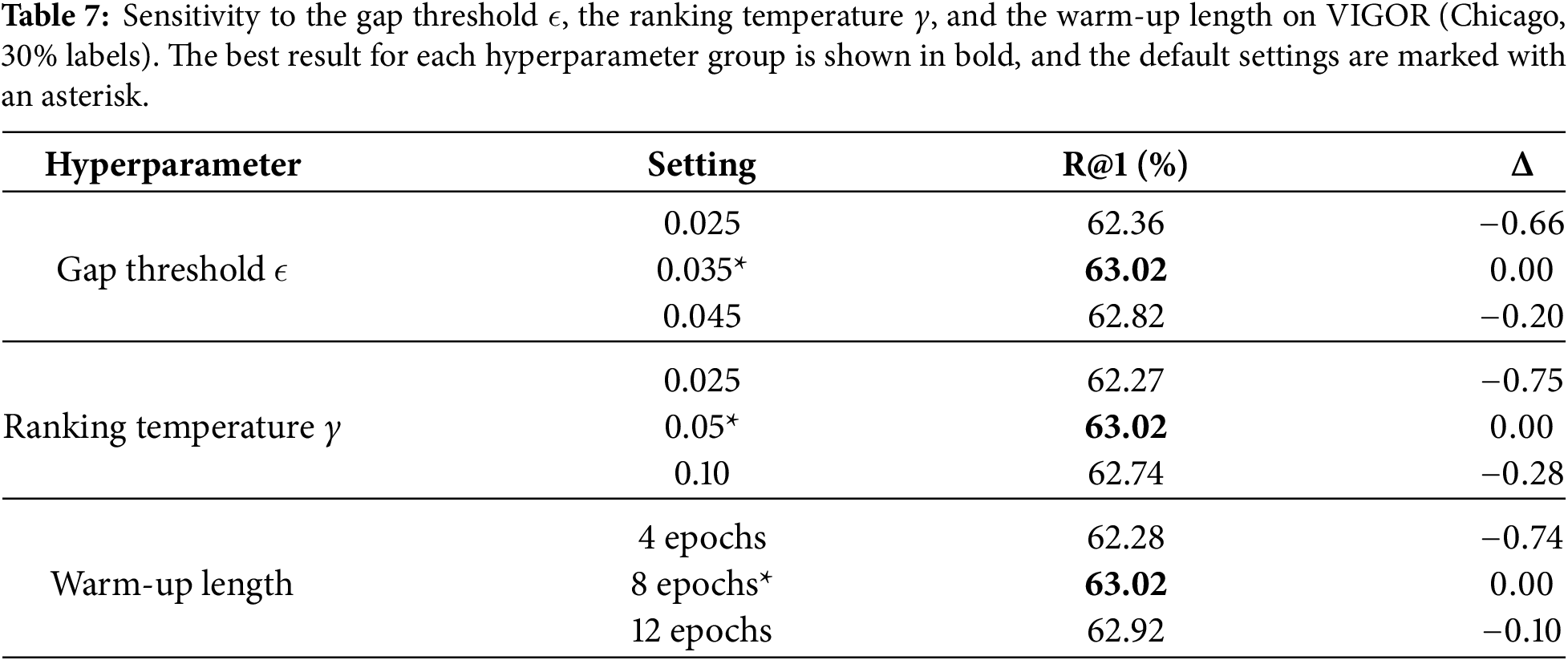
Gap threshold. We scan a window of ±0.01 around the value adopted in Section 4.1. The selected value ε=0.035 gives the best result, 63.02% R@1, and the largest drop inside the window is 0.66 percentage points. A smaller threshold more readily interprets a local similarity fluctuation as a breakpoint, whereas a larger one can skip a meaningful positive/negative boundary, so the intermediate value balances candidate coverage against reliability. Because all three settings stay within 62.36%–63.02%, the method does not depend on an exactly tuned single point. We do not claim a universal threshold that holds for every dataset, since the similarity scale varies with scene structure and gallery overlap; this is why ε is specified per dataset, and the subsequent mutual consistency check provides a second filter for candidates that occasionally cross the breakpoint by accident.

Ranking temperature and warm-up length. The ranking temperature controls how sharply the confidence mass is distributed inside a mined positive set. Values of 0.025, 0.05 and 0.10 give 62.27%, 63.02% and 62.74% R@1, a maximum difference of 0.75 percentage points, and γ=0.05 offers the best balance between emphasizing the most reliable positive and still using the remaining valid ones. Together with the uniform-weighting result of Table 5, which corresponds to the large-temperature limit, this indicates that the weighted objective is not sharply sensitive to this parameter. For the warm-up, extending it to 12 epochs still gives 62.92%, only 0.10 points from the default 8 epochs, so the model does not depend on a precise cut-off. Shortening it to 4 epochs lowers R@1 to 62.28%, which is consistent with the expectation that mining launched from an insufficiently converged representation is less reliable, although the decrease remains below one point. Eight epochs therefore provide a sufficiently mature initialization while allowing pseudo-label mining to begin early, rather than representing a fragile test-tuned cut-off.

Mining frequency. Pseudo labels are regenerated once per epoch in all experiments on CVUSA, CVACT and VIGOR, without any per-dataset adjustment. Changing this interval would simultaneously change the freshness of the pseudo labels, the total number of mining rounds, and the training budget, so we treat it as part of the alternating optimization protocol rather than as a dataset-specific tuning knob. Under this once-per-epoch protocol, the 91 consecutive rounds analyzed in Section 4.6 show that precision remains above 93% and that R@1 settles near 63% without evidence of error amplification, while the timing in Section 4.7 shows that mining occupies only 16.59% of a complete post-warm-up epoch. Updating every epoch therefore exploits the improved representation promptly at an acceptable cost.

4.6 Pseudo-Label Quality Analysis

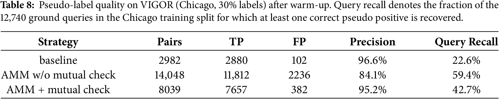
Since the framework depends on pseudo-label quality, we examine AMM on VIGOR (Chicago, 30% labels) right after warm-up, when the representation is weakest and mining most likely to make errors. A mined pair is counted as correct when the retrieved tile belongs to the annotated positive set of the query, that is, its primary tile or one of its three neighboring valid tiles. Table 8 compares three strategies along the precision–recall trade-off that governs iterative self-training. The mutual Top-1 baseline keeps precision high (96.6%) but recovers a correct positive for only 22.6% of the queries, leaving most unlabeled data unused. Dropping the reverse verification from AMM raises query recall to 59.4% but admits many false positives and lowers precision to 84.1%, which is harmful for iterative training because incorrect pseudo labels introduce biased gradients. The complete AMM, with the mutual consistency check as a built-in precision control, recovers 95.2% precision while retaining 42.7% query recall, delivering 7657 correct pseudo pairs, which is 2.66 times the number produced by the baseline. In addition, the true positives rejected by the check have a lower average similarity than those retained (0.376 vs. 0.414), confirming that it mainly removes ambiguous low-confidence matches. Since pseudo labels are regenerated every epoch, some low-confidence matches rejected early may be selected later after the representation improves.

Evolution over training. Because pseudo-label mining and model updating are performed alternately, we further examine how pseudo-label quality evolves during training and whether errors are progressively amplified. We record 91 consecutive mining rounds from epoch 9, the first epoch after warm-up, to epoch 99. Precision is defined as the number of correct accepted pairs divided by all accepted pairs, whereas pair recall is the number of correct accepted pairs divided by the 50,960 annotated positive pairs in the Chicago training split. Therefore, this pair-level recall differs from the query-level recall in Table 8, which only requires at least one correct positive for each query. Table 9 reports the two endpoints, while Fig. 3 presents the complete evolution curves.

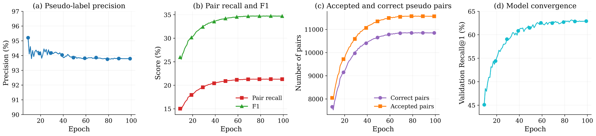
Figure 3: Evolution of pseudo-label quality and model convergence on VIGOR (Chicago, 30% labels): (a) pseudo-label precision, (b) pair recall and F1, (c) correct and accepted pseudo-label pairs, and (d) retrieval R@1 on the Chicago evaluation split. Pair recall, F1, and the number of correct pseudo-label pairs increase steadily, while precision remains above 93%. R@1 increases from 45.09% to 62.90% and remains stable at approximately 63% during late training.

Pseudo-label coverage expands steadily during training. The number of accepted pairs increases from 8039 to 11,567, while the number of correct pairs increases from 7657 to 10,849. Accordingly, pair recall improves from 15.03% to 21.29%, and F1 improves from 25.96% to 34.70%. Although precision decreases slightly from 95.25% to 93.79% as coverage expands, it remains above 93% throughout training and becomes stable after approximately epoch 60. Thus, no progressive precision collapse is observed.

R@1 increases from 45.09% at epoch 9 to 62.90% at epoch 99 and remains close to 63% during late training, rather than degrading as more pseudo-positive pairs are accepted. As coverage expands, the number of falsely accepted pairs also grows, from 382 at epoch 9 to 718 at epoch 99, so the absolute amount of label noise does increase. Precision nevertheless stays above 93% and retrieval accuracy does not deteriorate in the late stage. Because the pseudo-label sets are regenerated in each mining round instead of being accumulated permanently, an incorrectly accepted candidate is not necessarily retained in the following rounds. These observations therefore provide no evidence of progressive error amplification: the mutual consistency check expands positive-pair coverage while keeping precision high, and under the evaluated setting the residual pseudo-label noise does not prevent stable convergence.

4.7 Computational Overhead and Scalability

Because AMM adds reverse-consistency verification to pseudo-label mining, we compare the complete method with a single-positive variant under identical data, hardware, software, feature-extraction, and similarity-computation settings. The variant retains only one forward candidate and omits mutual verification. Unless stated otherwise, the times in Table 10 include feature extraction, similarity computation, and post-processing.

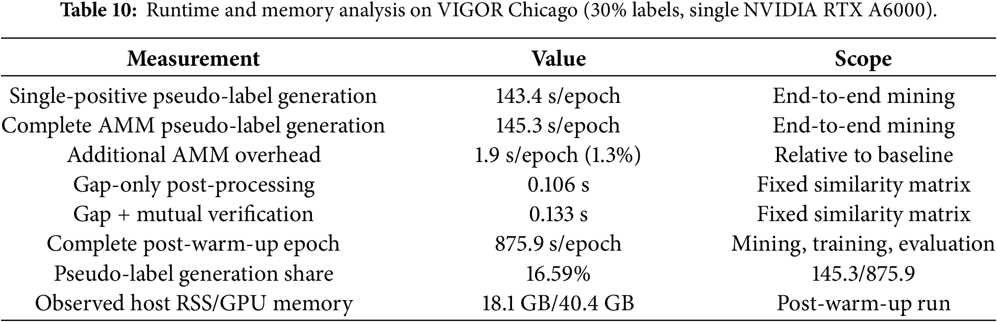
Complete AMM requires 145.3 s per mining round, compared with 143.4 s for the single-positive variant. Thus, mutual verification and multi-positive construction introduce approximately 1.9 s, or 1.3%, additional end-to-end mining time. Pseudo-label generation accounts for 16.59% of a complete post-warm-up epoch. With the similarity matrix fixed, adding mutual verification increases post-processing from 0.106 to 0.133 s. This increment is small because the reverse Top-1 matches are obtained from the same similarity matrix along its opposite dimension. Multi-positive training similarly reuses the existing in-batch logits and only constructs an additional positive mask and soft target distribution.

The dominant computational cost remains exact similarity computation. Let Nq denote the number of ground queries, Ns the gallery size, and D the descriptor dimension. Feature extraction scales linearly with Nq+Ns, while dense similarity computation requires O(NqNsD) time and O(NqNs) memory when the complete matrix is materialized. Extracting the ranked head of each query together with the reverse Top-1 matches requires a single pass whose cost scales approximately linearly with the size of the matrix. Breakpoint detection and mutual verification operate only on these retained candidates and therefore add negligible cost compared with feature extraction and similarity computation.

The 30% label setting changes the fraction of training queries with known correspondence labels, but AMM performs mining over all 12,740 ground queries in the Chicago training split. The resulting 12,740×12,740 FP32 similarity matrix occupies approximately 619 MiB. Comparing the same queries with the complete 22,308-tile Chicago gallery would require approximately 1.06 GiB. For substantially larger galleries, exact similarities can be computed blockwise while retaining only the leading candidates of each ranking and the reverse Top-1 state. This reduces peak memory without changing the asymptotic cost of exact similarity computation. Approximate nearest-neighbor indexing offers a possible further acceleration, but is not evaluated in this work.

4.8 Qualitative Retrieval Analysis

To look beyond overall recall, we visualize representative top-5 retrievals on VIGOR, where green and red boxes mark true and false positives according to the ground-truth positive set. Fig. 4 shows successful cases across industrial roads, vegetation-dominated residential areas, dense urban intersections, and open plaza-like areas. In these cases the model relies on shared spatial structure such as road layouts, building footprints, open regions, and vegetation. Multiple true positives often appear within the top-5. This supports the many-to-many setting of VIGOR and shows why single-positive training can be problematic. The highest-ranked tile is emphasized while the other valid tiles still contribute to the optimization instead of being repelled. Fig. 5 collects typical failures, driven mainly by repetitive transportation or industrial structures that produce near-identical candidates, dense-urban occlusions and shadows, vegetation that hides discriminative cues, and low-texture waterfronts that make different riverbank locations hard to tell apart. In most failures a true positive still appears at a lower rank, indicating fine-grained ranking ambiguity under weak or repetitive cues rather than a complete failure of the learned correspondence. This suggests that confidence-aware negative mining may be useful in future work.

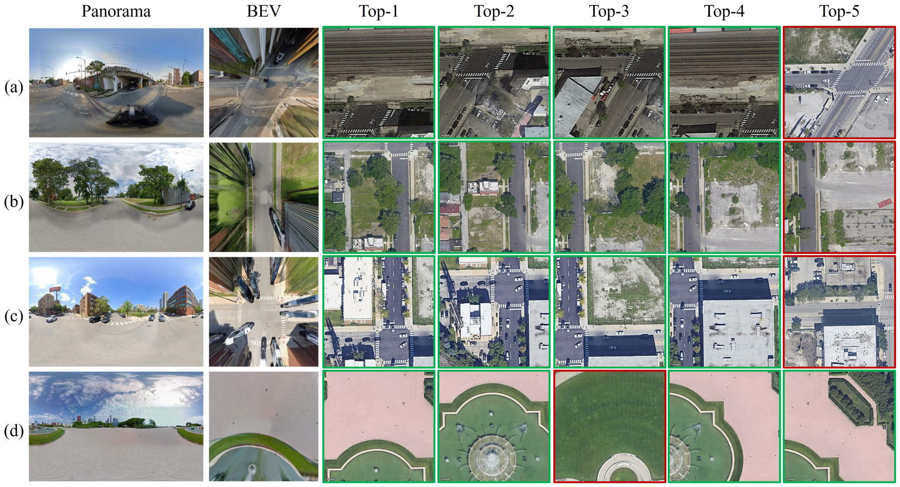
Figure 4: Successful top-5 retrieval examples on VIGOR. Each row is one ground panorama query, shown together with its BEV projection and its top-5 satellite retrievals; green boxes denote true positives and red boxes denote false positives. The four rows illustrate different scene types: (a) an industrial road and rail corridor; (b) a vegetation-dominated residential block; (c) a dense urban intersection; and (d) an open plaza-like area. In each case several geographically valid satellite candidates are retrieved within the top-5.

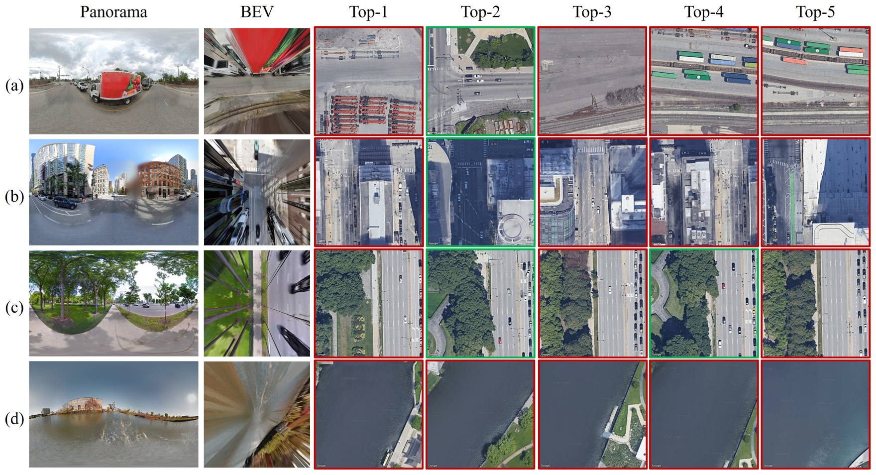
Figure 5: Representative failure cases on VIGOR, using the same layout as Fig. 4. The four rows illustrate the dominant failure modes: (a) repetitive transportation and industrial structures that produce near-identical candidates; (b) dense urban occlusions and shadows; (c) vegetation that hides discriminative cues; and (d) a low-texture waterfront in which different riverbank locations are hard to distinguish. Although the top-1 result is incorrect in these examples, a true positive still appears at a lower rank in most of them.

5  Conclusion

This paper studies semi-supervised ground-to-satellite geo-localization under realistic many-to-many correspondences. We show that one-to-one pseudo-labeling can miss valid positives and may treat true matches as negatives. The proposed DMP-Geo addresses this problem with a bird’s-eye fused query representation, adaptive breakpoint-based multi-positive mining with mutual consistency verification, and a confidence-weighted contrastive objective. Experiments on CVUSA, CVACT, and VIGOR show consistent improvements over the existing semi-supervised baseline under limited annotation budgets and strong generalization under the challenging VIGOR Cross-area protocol. The pseudo-label analysis further shows that DMP-Geo recovers more correct positive pairs while maintaining high precision and stable model convergence. Although the current evaluation covers bidirectional cross-dataset transfer and unseen-city testing, broader domain shifts involving weather, season, sensors, and geographic regions remain to be investigated. Future work will study these settings, confidence-aware negative selection, and meter-level fine-grained localization.

Acknowledgement: None.

Funding Statement: This work was supported by the National Natural Science Foundation of China (52405309), the Natural Science Foundation of Henan Province, China (252300421064), and the Henan Provincial Science and Technology Research Project (262102210190).

Author Contributions: The authors confirm contribution to the paper as follows: conceptualization, Long Yu and Ma Zhu; methodology, Long Yu; software, Long Yu; validation, Long Yu, Ma Zhu and Xu Wang; formal analysis, Long Yu and Yang Pei; investigation, Long Yu and Xu Wang; resources, Ma Zhu; data curation, Long Yu and Chunfang Yang; writing—original draft preparation, Long Yu; writing—review and editing, Ma Zhu, Xu Wang, Yang Pei and Chunfang Yang; visualization, Long Yu; supervision, Ma Zhu; project administration, Ma Zhu; funding acquisition, Chunfang Yang. All authors reviewed and approved the final version of the manuscript.

Availability of Data and Materials: The three benchmark datasets used in this study—CVUSA, CVACT, and VIGOR—are publicly available, and the implementations of the compared methods can be obtained from the links provided in their respective original publications. The BEV preprocessing uses the publicly released UCVGL GeometricProjection implementation. We report the exact projection geometry, the dataset-specific field-of-view values and their sources or rationale, the provenance of the ε values, the training hyperparameters, and pseudocode for the mining procedure. The source code developed in this study is not currently publicly available owing to ongoing follow-up research, but further methodological details are available from the corresponding author upon reasonable request.

Ethics Approval: Not applicable.

Conflicts of Interest: The authors declare no conflicts of interest.

References

1. Mithun NC, Minhas KS, Chiu HP, Oskiper T, Sizintsev M, Samarasekera S, et al. Cross-view visual geo-localization for outdoor augmented reality. In: Proceedings of the 2023 IEEE Conference on Virtual Reality and 3D User Interfaces (VR); 2023 Mar 25–29; Shanghai, China. p. 493–502. [Google Scholar]

2. Li A, Hu H, Mirowski P, Farajtabar M. Cross-view policy learning for street navigation. In: Proceedings of the 2019 IEEE/CVF International Conference on Computer Vision (ICCV); 2019 Oct 27–Nov 2; Seoul, Republic of Korea. p. 8099–108. [Google Scholar]

3. Häne C, Heng L, Lee GH, Fraundorfer F, Furgale P, Sattler T, et al. 3D visual perception for self-driving cars using a multi-camera system: calibration, mapping, localization, and obstacle detection. Image Vis Comput. 2017;68(1):14–27. doi:10.1016/j.imavis.2017.07.003. [Google Scholar] [CrossRef]

4. Workman S, Souvenir R, Jacobs N. Wide-area image geolocalization with aerial reference imagery. In: Proceedings of the 2015 IEEE International Conference on Computer Vision (ICCV); 2015 Dec 7–13; Santiago, Chile. p. 3961–9. [Google Scholar]

5. Shi Y, Liu L, Yu X, Li H. Spatial-aware feature aggregation for image based cross-view geo-localization. In: Proceedings of the 33rd International Conference on Neural Information Processing Systems; 2019 Dec 8–14; Vancouver, BC, Canada. Red Hook, NY, USA: Curran Associates, Inc.; 2019. p. 10090–100. [Google Scholar]

6. Yang H, Lu X, Zhu Y. Cross-view geo-localization with layer-to-layer transformer. In: Proceedings of the 35th International Conference on Neural Information Processing System; 2021 Dec 6–14; Virtual. Red Hook, NY, USA: Curran Associates, Inc.; 2021. p. 29009–20. [Google Scholar]

7. Zhu S, Shah M, Chen C. TransGeo: transformer is all you need for cross-view image geo-localization. In: Proceedings of the 2022 IEEE/CVF Conference on Computer Vision and Pattern Recognition (CVPR); 2022 Jun 18–24; New Orleans, LA, USA. New York, NY, USA: IEEE; 2022. p. 1152–61. [Google Scholar]

8. Zhang X, Li X, Sultani W, Zhou Y, Wshah S. Cross-view geo-localization via learning disentangled geometric layout correspondence. Proc AAAI Conf Artif Intell. 2023;37(3):3480–8. doi:10.1609/aaai.v37i3.25457. [Google Scholar] [CrossRef]

9. Zhang X, Li X, Sultani W, Chen C, Wshah S. GeoDTR+: toward generic cross-view geolocalization via geometric disentanglement. IEEE Trans Pattern Anal Mach Intell. 2024;46(12):10419–33. doi:10.1109/tpami.2024.3443652. [Google Scholar] [CrossRef]

10. Chen Z, Yang ZX, Rong HJ, Li G. Without paired labeled data: end-to-end self-supervised learning for drone-view geo-localization. IEEE Trans Neural Netw Learn Syst. 2026. doi:10.1109/tnnls.2026.3696684. [Google Scholar] [CrossRef]

11. Li H, Xu C, Yang W, Yu H, Xia GS. Learning cross-view visual geo-localization without ground truth. IEEE Trans Geosci Remote Sens. 2024;62:1–17. doi:10.1109/tgrs.2024.3425608. [Google Scholar] [CrossRef]

12. Li H, Xu C, Yang W, Mi L, Yu H, Zhang H, et al. Unsupervised multiview UAV image geolocalization via iterative rendering. IEEE Trans Geosci Remote Sens. 2025;63:1–15. doi:10.1109/tgrs.2025.3572710. [Google Scholar] [CrossRef]

13. Li G, Qian M, Xia GS. Unleashing unlabeled data: a paradigm for cross-view geo-localization. In: Proceedings of the 2024 IEEE/CVF Conference on Computer Vision and Pattern Recognition (CVPR); 2024 Jun 16–22; Seattle, WA, USA. New York, NY, USA: IEEE; 2024. p. 16719–29. [Google Scholar]

14. Zhu S, Yang T, Chen C. VIGOR: cross-view image geo-localization beyond one-to-one retrieval. In: Proceedings of the 2021 IEEE/CVF Conference on Computer Vision and Pattern Recognition (CVPR); 2021 Jun 20–25; Nashville, TN, USA. New York, NY, USA: IEEE; 2021. p. 5316–25. [Google Scholar]

15. Hou S, Qin Z, Wu C, Yin G, Wang X, Wang Z. DIEONet: domain-invariant information extraction and optimization network for visual place recognition. Comput Mater Contin. 2025;82(3):5019–33. doi:10.32604/cmc.2025.058233. [Google Scholar] [CrossRef]

16. Xiang L, Fu H, Yang C. CerfeVPR: cross-environment robust feature enhancement for visual place recognition. Comput Mater Contin. 2025;84(1):325–45. doi:10.32604/cmc.2025.062834. [Google Scholar] [CrossRef]

17. Zhang Q, Zhu Y. Aligning geometric spatial layout in cross-view geo-localization via feature recombination. Proc AAAI Conf Artif Intell. 2024;38(7):7251–9. doi:10.1609/aaai.v38i7.28554. [Google Scholar] [CrossRef]

18. Huang J, Wu M, Li P, Wu W, Yu R. VimGeo: efficient cross-view geo-localization with vision mamba architecture. In: Proceedings of the Thirty-Fourth International Joint Conference on Artificial Intelligence; 2025 Aug 16–22; Montreal, QC, Canada. p. 1188–96. [Google Scholar]

19. Zheng Z, Wei Y, Yang Y. University-1652: a multi-view multi-source benchmark for drone-based geo-localization. In: Proceedings of the 28th ACM International Conference on Multimedia; 2020 Oct 12–16; Seattle, WA, USA. New York, NY, USA: ACM; 2020. p. 1395–403. [Google Scholar]

20. Fan J, Yang X, Lu R, Li Q, Wang S. Multi-modal scene matching location algorithm based on M2Det. Comput Mater Contin. 2023;77(1):1031–52. doi:10.32604/cmc.2023.039582. [Google Scholar] [CrossRef]

21. Wang T, Zheng Z, Yan C, Zhang J, Sun Y, Zheng B, et al. Each part matters: local patterns facilitate cross-view geo-localization. IEEE Trans Circuits Syst Video Technol. 2022;32(2):867–79. doi:10.1109/tcsvt.2021.3061265. [Google Scholar] [CrossRef]

22. Tian X, Shao J, Ouyang D, Shen HT. UAV-satellite view synthesis for cross-view geo-localization. IEEE Trans Circuits Syst Video Technol. 2022;32(7):4804–15. doi:10.1109/tcsvt.2021.3121987. [Google Scholar] [CrossRef]

23. Shen T, Wei Y, Kang L, Wan S, Yang YH. MCCG: a ConvNeXt-based multiple-classifier method for cross-view geo-localization. IEEE Trans Circuits Syst Video Technol. 2024;34(3):1456–68. [Google Scholar]

24. Wang X, Zhang L, Fan Z, Liu Y, Chen C, Deng F. From coarse to fine: a matching and alignment framework for unsupervised cross-view geo-localization. Proc AAAI Conf Artif Intell. 2025;39(8):8024–32. [Google Scholar]

25. Xie K, Zhou W, Huang X, Guan H, Yulong F. Self-supervised cross-view graph search framework for ground-to-satellite geo-localization. IEEE Trans Geosci Remote Sens. 2025;63(86):1–14. doi:10.1109/tgrs.2025.3602685. [Google Scholar] [CrossRef]

26. Khosla P, Teterwak P, Wang C, Sarna A, Tian Y, Isola P, et al. Supervised contrastive learning. In: Proceedings of the 34th International Conference on Neural Information Processing System; 2020 Dec 6–12; Vancouver, BC, Canada. p. 18661–73. [Google Scholar]

27. Wang X, Han X, Huang W, Dong D, Scott MR. Multi-similarity loss with general pair weighting for deep metric learning. In: Proceedings of the 2019 IEEE/CVF Conference on Computer Vision and Pattern Recognition (CVPR); 2019 Jun 15–20; Long Beach, CA, USA. p. 5017–25. [Google Scholar]

28. Miech A, Alayrac JB, Smaira L, Laptev I, Sivic J, Zisserman A. End-to-end learning of visual representations from uncurated instructional videos. In: Proceedings of the 2020 IEEE/CVF Conference on Computer Vision and Pattern Recognition (CVPR); 2020 Jun 13–19; Seattle, WA, USA. p. 9876–86. [Google Scholar]

29. Dwibedi D, Aytar Y, Tompson J, Sermanet P, Zisserman A. With a little help from my friends: nearest-neighbor contrastive learning of visual representations. In: Proceedings of the 2021 IEEE/CVF International Conference on Computer Vision (ICCV); 2021 Oct 10–17; Montreal, QC, Canada. p. 9568–77. [Google Scholar]

30. Huynh T, Kornblith S, Walter MR, Maire M, Khademi M. Boosting contrastive self-supervised learning with false negative cancellation. In: Proceedings of the 2022 IEEE/CVF Winter Conference on Applications of Computer Vision (WACV); 2022 Jan 3–8; Waikoloa, HI, USA. p. 2785–95. [Google Scholar]

31. Wang X, Xu R, Cui Z, Wan Z, Zhang Y. Fine-grained cross-view geo-localization using a correlation-aware homography estimator. In: Proceedings of the 37th International Conference on Neural Information Processing Systems; 2023 Dec 10–16; New Orleans, LA, USA. Red Hook, NY, USA: Curran Associates, Inc.; 2023. p. 5301–19. [Google Scholar]

32. Liu L, Li H. Lending orientation to neural networks for cross-view geo-localization. In: Proceedings of the 2019 IEEE/CVF Conference on Computer Vision and Pattern Recognition (CVPR); 2019 Jun 15–20; Long Beach, CA, USA. New York, NY, USA: IEEE; 2019. p. 5617–26. [Google Scholar]

33. Liu Z, Mao H, Wu CY, Feichtenhofer C, Darrell T, Xie S. A ConvNet for the 2020s. In: Proceedings of the 2022 IEEE/CVF Conference on Computer Vision and Pattern Recognition (CVPR); 2022 Jun 18–24; New Orleans, LA, USA. New York, NY, USA: IEEE; 2022. p. 11966–76. [Google Scholar]