Q-Learning-Based Pesticide Contamination Prediction in Vegetables and Fruits

1  Introduction

In agricultural production, pesticides are frequently utilized as they aid in the prevention of insects and illnesses, as well as the increase of harvests in agriculture. Pesticides in this category are indeed a mixture of elements, including chemical or biological factors, which are meant to resist, kill, or manage any pest, or even modulate plant development. Due to their capacity to permeate vegetable tissues, widespread use of these pesticides has the potential to cause considerable long-term environmental change and damage. As a result of the negative consequences caused by pesticide residue, there is now a global concern about pesticide usage in farming [1]. However, pesticides are sometimes used inappropriately, which can result in pesticide residues as well as serious pollution of the environment. Pesticides might be categorized by chemical structure, which along with carbonate, organ phosphorus, pyrethroids, organ chlorine, heterocycles, as well as amides, for their utilization in farming [2]. Global vegetable consumption has gradually grown, possibly as a result of rising income levels and increased knowledge of the significance of a well-balanced diet. With the rising demand for fresh vegetables and fruits, the use of agricultural pesticides would surely be in line with population expansion [3]. Thus, some methods have been introduced to measure the freshness of vegetables and fruits with regard to pesticide residue. Codex Aliment Arius Commission (Codex) techniques have also utilized a method devised by the Collaborative FAO (Food and Agriculture Organization)/WHO (World Health Organization) Gathering on Pesticide Residues (JMPR- Joint Meeting on Pesticide Residues) to observe the exact allowable maximum amount of such a pesticide residue that could legitimately be contained in or on food. Also, the maximum residue level (MRL), which is stated in mg/kg, is the accepted safe limit [4]. Similarly, MRL is determined by the quantitative measurement of a specific active component found in food samples with essential Good Agricultural Practices (GAP). Even when pesticides are used in accordance with local agricultural laws, a trace amount of pesticide residue or metabolite may be found in some crops. Pesticide monitoring and regulation are carried out with various analytical methods to verify whether pesticide residual concentrations in food items are below the allowed limit [5]. This includes any pesticide derivatives that are toxicologically or Eco toxicologically important, including transformation as well as degradation byproducts, metabolites, and reactive products, including contaminants. It is no longer used because potential acute toxic effects following chronic or sub-chronic pesticide exposure are not typically addressed during the human health risk assessment stage [6]. As a result, a technique for measuring pesticide contamination was implemented in most applications to address this critical issue by establishing a value based on the pesticide’s acute effects [7].

Mass spectrometry (MS) was probably one of the most frequently used confirmation methods to predict pesticide residue levels during the risk assessment stage [8]. To get mass spectrometry, it first detaches that material’s particles into ions of diverse masses. It then leverages the differential mobility behavior of ions in an electric as well as a magnetic field to distinguish the ions depending mostly on mass charge ratio. The data may be used to acquire qualitative and quantitative information about the pesticide residues as it focuses on the sample’s molecular structure [9]. Moreover, such systems confront the usual problem of processing just a limited number of samples as well as a large set of information input dimensions, which creates difficulties. As a result, deep learning would directly retrieve characteristics from raw, high-dimensionality data by learning data attributes. As a consequence, this was examined if mass spectral information might be utilized to determine molecular substructure. Since the development of deep learning, various systems based on recurrent neural networks have exhibited incredible promise when dealing with the problem in preprocessing of the sequence data stream [10]. To measure and match the chemical molecular patterns of the pesticide residue, some methods have been proposed, such as plant disease net and Alex Net CNN. Unfortunately, these techniques failed to identify both sequential and spatial data, despite the fact that pesticide residue contamination measurements at the soil level are also required to anticipate and decrease the dangerous level to the environment. In real-world applications, researchers seldom come across anything more complicated than disjunctions between different event kinds, like measuring pesticide contamination by matching it with fertilizers, image-level prediction of pesticides, and their harmfulness to the environment. The reason for this is that the remainder is difficult to comprehend, and maintaining algebraic rules in event specification applications such as pesticide detection is difficult. Early detection of sequences of events is necessary, in which a fault is any sequence that is not followed by the next event in the series within a time limit or that another event type occurs later in the sequence, which is the biggest and most complicated event expression. A framework is required that must integrate data from a variety of sources to create events or patterns, allowing properties to define, manage, and forecast events, situations, and possible risks of pesticide level.

Complex Event Processing (CEP) is a new technique that examines, filters, and combines conceptually low-level events to identify complex occurrences [11,12] in the data stream. This complex event stream processing technique assists a user in concluding data gathered from many samples like soil, water, and air. The ultimate objective of these technologies is to discover hard-to-find opportunities or dangers in high-volume, fast-happening events from several fields and sources. CEP systems continuously collect data from a variety of sources about raw events in system operations [13] and use algorithms and rules to discover the linked trends and patterns that combine them into complex events in real-time, such as finding residue level, finding compounds, and surface defect assessment, which were difficult to perform using machine learning techniques [14]. The findings are subsequently forwarded to the relevant user. A fundamental goal underlying CEP systems seems to be to recognize situations in authentic time through evaluating the causal interconnections among simple occurrences that contain no special information under stand-alone circumstances. As a consequence of such an evaluation, real-time warnings concerning the identification of complicated processes have been sent to decision-makers, controlling this same situation preemptively and responding flexibly in reaction to evolving conditions. Both precision, as well as timeliness of decision-making, are often utilized to assess the efficacy and usefulness of CEP systems.

The major contributions of the proposed design are as follows:

1.    To minimize and effectively use pesticides in the agricultural field and also ensure the safety of farmers and consumers,

2.    By evaluating the use of pesticides, intensity, and types of pesticides with their percentage level, an objective function will be created to ensure the maximum threshold level.

3.    Setting up event generation in CEP to produce the best results in real-time pesticide level measurements.

By considering the above-stated objectives as major ones, a proposed model will be designed and its results will be examined.

The remainder of this paper has been formatted as follows: Section 2 offers a summary of the literature review section, while Section 3 describes the proposed approach. Section 4 details the experimental findings, while Section 5 concludes the research as a whole.

2  Literature Review

Many techniques have been proposed previously to find pesticide contamination in soil. Some of them are reviewed with their drawbacks below.

EL-Saeid et al. [15] have presented a method of pesticide contamination to obtain residue levels from the soil. It gathered samples of soil from Al-Kharj Governorate in Saudi Arabia, which seems located southeast near Riyadh. To generate residue intensity assessments, an investigation of the Al-Kharj farming region of 14 pesticide residues about organochlorine pesticide (OCPs), organophosphorus pesticide (OPPs), pyrethroids, carbamates, as well as biopesticides was conducted. Residues such as Spinosad, chlorpyrifos-methyl, etc were discovered in the soil. Extensive modeling on large as well as also small scale, especially catchment-level assessments, on the other hand, is not reported. Devi et al. [16] created a system prototype that detected pesticides using four sensors (temperature, gas, pH, and moisture), an Arduino microcontroller, and a Wi-Fi module. Pesticides are regarded to be present in a fruit if pesticides are detected in a range above or below the MRL. The content of pesticides and data acquired from each sensor via the Internet of Things (IoT). The sickness afflicting the fruit is found and stored once deep Learning is applied to the image of the fruit.

Malaj et al. [17] presented pesticide utilization regarding three significant kinds of pesticides: herbicides, fungicides, as well as insecticides. This created the Wetland Pesticide Incidence Rating, which integrates spatially distributed data concerning pesticide usage densities, wetland density, rainfall, plus contaminant physicochemical attributes to assess potential wetland exposure. Pesticide utilization varied by province, however, the principal pesticides being used are constant across the area but were also connected with wheat as well as canola plants. Chavez Rodriguez et al. [18] developed gene-centric frameworks of combined microbial dynamics as well as pesticide degradation relying on assessments of genetic abundance & function. Utilizing such an informative paradigm towards genetic data. This was evaluated as well as acknowledged through two batch procedures which deteriorated the pesticide dichlorophenoxyacetic acid. Considering pesticide-induced gene expression, on either hand, results in below-average efficiency in tracking microbial dynamics as well as forecasting pesticide mineralization. Silva et al. [19] developed a strategy for predicting pesticide concentrations in soil that were consistent with application data, well with the greatest concentrations in dry pulses-vegetables-flowers as well as in Southern Europe. Especially compared with observed data, forecast-based thresholds resulted through comparatively small soil health. Nevertheless, the findings emphasize the requirement of tracking pesticide residue surveillance activities in soil, as well as appropriate risk management assessment strategies for mixes, and also the necessity to define pesticide threshold approaches.

DiGiacopo et al. [20] suggested research to investigate environmental settings wherein plasticity is likely to be favorable or destructive. It discovered that whenever pesticides were absent, greater plastic populations displayed lower pesticide tolerance but were healthier over less plastic populations, presumably to minimize the expense of exhibiting high tolerance when that wasn’t necessary. Unfortunately, it was a sophisticated evaluation technique that failed to identify pesticide threshold methods.

Tang et al. [21] established an electronic nose approach for the detection of parathyroid in tea. This same article examined a collection of metal oxide sensors with a portable electronic nose (PEN 3) electronic nose but also discovered that four of them seem to be appropriate for detecting the very same parathyroid pesticide with diversified concentrations. This makes use of neural network methodology centered on back-propagation (BP). Unfortunately, the precision among those designs fell short of perfection. Bhandari et al. [22] reported a decreased number of pesticide residues as well as their lowest concentrations within soil samples taken from IPM farms. Their focus has been on Dichlorodiphenyltrichloroethane (DDT) contamination, and or the Stockholm Conference, a United Nations declaration, was indeed established. However, this model failed to reach the required level of prediction rate that was most necessary in the field of pesticide contamination. Blankson et al. [23] examined 21 pesticides in provided soil samples, and 17 of them were identified with varied frequencies in the tested samples, typically greater than 1%. Pesticide residues were found in 52 percent of the samples examined. The monitoring revealed that 20.0 percent of the samples were found to violate MRLs, while 32 percent of the samples had values that were below the MRL. However, this mathematical model implies that pesticide residue changes in vegetables should be monitored on a frequent, thorough, and periodic basis, with necessary steps that increased its complexity. Allen et al. [24] found that the number of identifiable pesticides, as well as the ratio of pesticide-contaminated crop samples, is significantly greater for those crops which are primarily grown in protected areas. These findings are greatest for crops obtained from enclosed cages, by which they have the most assurance. In comparison to the secured crop, analogous crops produced mostly in open fields have fewer pesticide residues as well as lower mean quantities of photo labile pesticides. Furthermore, in the crop combinations cabbage vs. lettuce as well as strawberries vs berries, that wasn’t the more evident. Zhu et al. [25] demonstrated a typical silver mirror process at room temperature to manufacture a D-SERS (Dynamic-surface-enhanced Raman scattering) substrate premised on a silver nanoparticles (Ag NP)-based standard laboratory filtration. In contrast to inexpensive, easy processing, as well as mass production, this substrate functions as a rag and also has great sample collecting effectiveness by easily swabbing over real-world surfaces. Due to its limited sensitivity and repeatability, this technique was coupled with paper substrates. Using Support Vector Machine and IoT, Madhav et al. [26] proposed a novel approach for predicting pesticides that humans consume and identifying illnesses in fruits.

Thus, by reviewing the methods discussed above it has been clear that there are some drawbacks such as lengthy measurement and frequent monitoring. Real-world applications mostly require a large quantity of information for processing. Thus to overcome this drawback a pesticide contamination prediction technique is required with the most probable results that have concern on consumer health.

3  A Hybrid Chronic Multi-Residual Framework

The rapid increase of vegetable yield while minimizing consumption, notably pesticide misuse. Pesticides are seen as a crucial aspect of modern farming, serving an important role in sustaining high crop yields. Pesticide residues in agricultural goods, both primary and secondary, represent significant health concerns to consumers. Pesticides produce long-term adverse impacts on both the environment as well as people’s health. Pesticide residues were ubiquitous in all plant production, however, exposure to residues in major agricultural products such as veggies and fruits causes the greatest health hazard. As a result, the growing of vegetables and fruits demands the invention of a model that measures and determines the levels of pesticide be applied to decrease human health hazards. Thus, in this article, an HCMF based on Q-learning with RNN is provided. The HCMF model analyses the pesticide based on the proportion of contamination that has been analyzed to assure the diagnosis of its range in soil, vegetables, and fruits. A Q-learning-based RNN was utilized in this research to predict pesticide levels in soil, vegetables, and fruits by assessing their maximum and lowest residual limit of pesticides. To anticipate this pesticide residue contamination level, complex Event Processing has been used and is being done for decision-making reasons to reduce and effectively utilize the pesticide in the Agri- Products.

The HCMF model analyses the pesticide based on its contamination level, which is then analysed to validate the identification of its range in soil, vegetables, and fruits, as illustrated in Fig. 1. To determine the permissible limit of the pesticide residue, MRL levels of phosphorous, magnesium, potassium, temperature, humidity, and moisture were extracted from the pesticide. The following section provides a brief overview of the HCMF model, which is used to forecast pesticide contamination levels in agricultural products and soil.

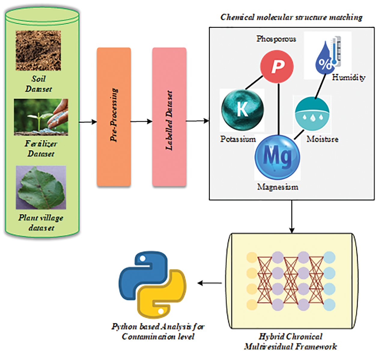
Figure 1: Block diagram of the overall proposed architecture

3.1 Prediction of Residue in Vegetables Fruits and Soil

Prediction of residue level is required to determine the count of pesticides contained in agricultural goods based on MRL. MRLs can be discovered in the online Codex pesticides in the agriculture database. The pesticide database may be searched by common name or class, as well as commodity name or code. To establish a long-term forecast of HCMF, data between 0.2 and 0.8 were standardized. Utilizing the Eq. (1)

Normalized,X=C1Xi−XminXmax−Xmin+C2 (1)

Consequently, Xmax represents the greatest amount of MRL, while Xmin symbolizes the lower limit of MRL. C1 And C2 are two constant values that were set in the range around 0.6. The collected values were then processed to be sequential ones for categorization purposes. After this procedure, multi-residue classes are created, which may subsequently be used to determine the maximum pesticide residue contamination level.

Complex Event Processing (CEP) was used to obtain these contamination values since it computes contamination levels using RNN with Q-Learning and makes judgments by producing events based on the MRL permissible limit. To identify the presence of pesticides in agricultural goods, HCMF employs a CEP filtering process that was anticipated using criteria such as high temperature, less humidity, moisture, and excessive phosphorus level, as well as a lower nitrogen level, all of which create residue levels. The existence of abnormality has provided input on whether the supplied Agri product is fertile or non-fertile, which characterizes the harmfulness of the MRL level. The information on pesticide levels has become more complicated due to the chemical patterns of presenting pesticides in Agri goods that must be augmented with historical pesticide levels, and this data most likely requires retrieval from each class label such as fertile or not. As a result, each incoming data point is compared to the stored fertilizer value, and HCMF creates a metric to make a choice. The forecast was made by filtering the data that was expected to be polluted by the herbicide.

To determine the MRL limit, normalization was conducted, and the final values were checked for contamination by comparing them to normal values. These prediction findings will be useful in the following stage, which will analyse its specificity. The next section explains the measurement of contamination levels in agricultural goods were determined using RNN-Q learning.

3.2 Measuring the Levels of Contamination in Vegetables, Fruits, and Soil using Q-Learning based RNN

The Q-Learning method is intuitively composed of learning a Q-table that represents the predicted future reward for each condition and action and the Q-table, which includes the Q-values of each state-action combination that has been iterated using the Q-value iteration. The Q-learning approach works effectively for finite states and actions spaces since storing every state-action combination would need a large amount of memory and many iterations for the Q-table to converge. It is simply impossible to utilize the Q-learning method when states space, actions space, or both are continuous. As a solution, we may calculate the Q-value function using Recurrent Neural Networks, which are well-known for their ability to estimate functions.

Consider the Q-table to be an assessment of an unknown function at certain places. Because it is a function, we can use Recurrent Neural Networks to estimate it, allowing us to work with uninterrupted spaces without difficulty.

When dealing with a complicated environment with several options and outcomes, the standard Q-learning process soon becomes inefficient. So, in this effort, we concluded combining the Deep Learning idea with Q learning and developing the Q Learning-based RNN. The Fig. 3 below illustrates the notion of Q learning-based RNN. It mostly entails constructing and training a neural network capable of calculating, given a state, the various Q-values for each action.

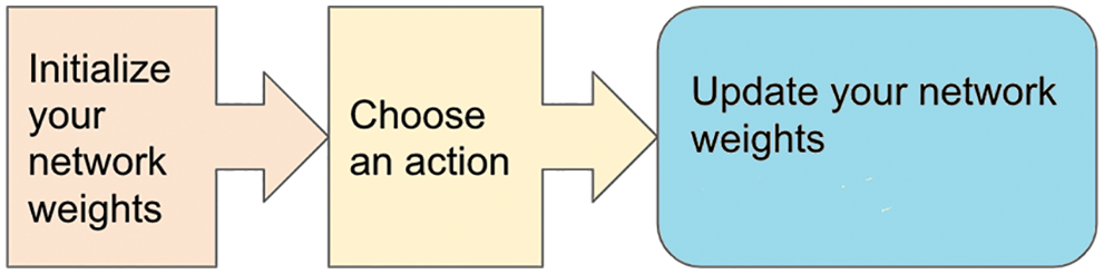
Figure 2: RNN with Q learning algorithm

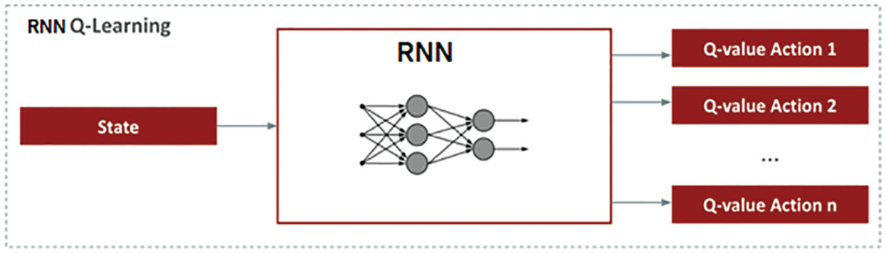
Figure 3: Q learning-based RNN model [27]

Stages for the Agent to learn the Q-table

1. To begin, a Q-table is arbitrarily initialized. The column counts reflect the number of activities whereas the count of rows denotes the state numbers that may be taken.

2. Then, as long as the episode isn’t finished:

2.1. In states, the agent chooses the action that maximizes the predicted rewards according to the Q-table.

2.2. In rare instances, the Agent is offered the choice of performing a random action. This is known as the epsilon greedy strategy. It enables the Agent to explore his environment when the epsilon rate falls. During the exploration phase, the agent gradually gains confidence in estimating the Q- values. Using the Bellman equation, the estimated new Q-values for being at the start and traveling right.

2.3. The Agent monitors the result state’s and the reward r, as well as modify the function Q (st, at) as regards:

QNew(St,at)=Q(St,at)+δ(rt+γ.maxQ(St+1,a)−Q(St,at) (2)

where, Q(St,at) = old Q-Value, rt -Rewards, γ -Discount Factor, δ -Learning Rate, QNew(St,at) -New Q value. This process is repeated indefinitely until the learning stops. The Q-Table is thus updated, and the value function Q is maximized and Q (state, action) provides the predicted future payoff of that action at that state in this case.

The RNN is fed a state as well as returns the Q-values among all possible actions for such a state. We understand that the RNN’s input layer is the same size as a state and that the output layer is the same size as the number of actions that the agent may do.

To summarize, when the agent reaches a specific state, he sends it through the RNN and selects the action with the greatest Q-value.

RNN-based Q-Learning presents two new techniques that allow for improved performance.

1 Memory Replay:

a) The neural network is not instantaneously updated after each step. Rather, it records each encounter in a memory.

b) The modifications are then performed towards a mini-batch comprising tuples drawn at arbitrary as from replayed memory.

c) Employing this way, the algorithm can recall as well as maintain track of his previous encounters.

2 Target Network Separation:

a) Using the same network to compute both the anticipated and goal values can cause significant instabilities.

b) To address this issue, it is frequently appropriate to train two distinct networks with the same architecture: a prediction network and a target network.

c) The prediction network operates as an “active” network, whereas the target network is a duplicate of the prediction network with frozen parameters that are updated regularly.

To estimate the objective, we may utilize a different network. The design of this target network is the same as that of the function approximator, but the parameters are fixed. After every cycle, all parameters from the predictive network were passed to the targeted system. These findings are in more steady training since the goal function remains constant.

Steps Involved in RNN based Q Learning Network and illustrated in Fig. 5:

1. Preprocess the states in the Q-Table then feed them into our proposed Q Learning-based RNN, which can return exact Q-values for all possible activities throughout the state.

2. Damaged leaf images have been chosen randomly.

3. Depending on the epsilon-greedy strategy, select action. We randomly pick the action with epsilon probability as well as a maximal Q-value action having 1-epsilon probability.

4. To obtain a reward, do the action in state s and then go to the next states. This stage contains a preprocessed image of the subsequent action stage. This transition has been stored in our replay buffer.

5. Following that, choose several random batches of transitions from the replay buffer and compute the loss.

6. Loss=(rt+γ.maxQ(St+1,a)−Q(St,at)2 Described in Fig. 4.

rt – Rewards, γ - Discount Factor, δ - Learning Rate, Q(St,at) - Q value at state S and St+1−Nextstate

7. To reduce this loss, use gradient descent concerning our real network parameters.

8. After each cycle, transform our actual network weights into target network weights.

9. Repeat these instructions for the desired number of episodes and a total reward has been obtained.

10. A new layer has been added that outputs the new Q value.

11. Finally, the Agent provides the contamination levels of the Agri products.

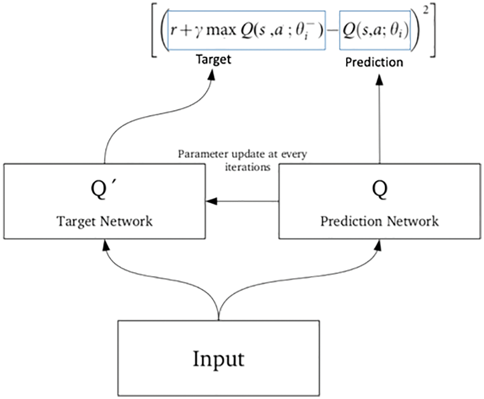
Figure 4: Loss function

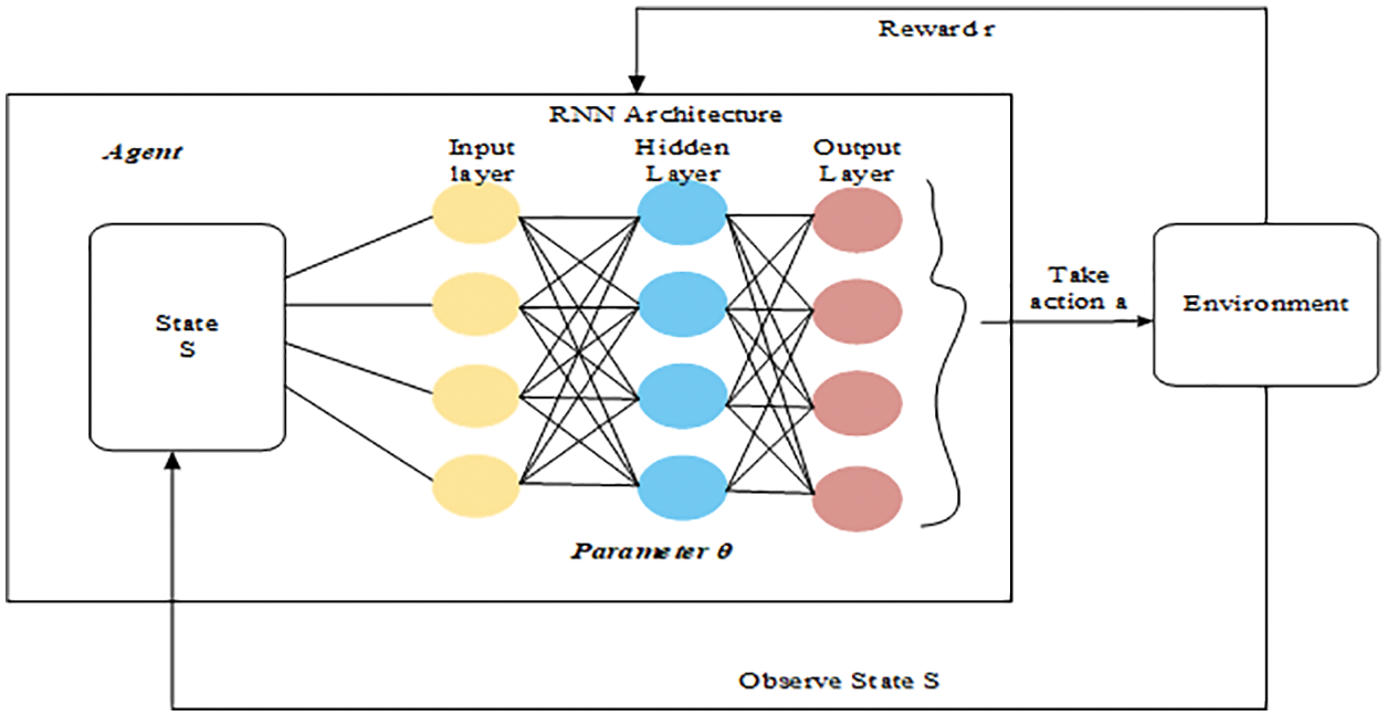
Figure 5: Schematic representation of Q-learning based RNN

To measure the contamination levels of the pesticide Agri products, RNN based on Q learning has been utilized. The level of contamination has been evaluated using many types of spectrometers in existing works. However, a limited number of pesticides has been evaluated. To evaluate the number of pesticides that are present in Agri products, Q-based RNN has been utilized in which the states such as total Reward has been found. By optimally applying the Q learning with supervised learning that optimizes parameter θ in a combined manner.

Fig. 6 depicts the flow process of RNN training based on Q learning. Similarly, the training procedure is divided into two parts. The initial stage is just to train that RNN, followed by training the agent therein environment. Based on a rule-based policy, the agent chooses and executes an action. In this case, the action is chosen at random with the lowest probability, but the probability selects the action with the highest q value. A gradient descent approach was used, which iteratively modifies the weights in the network according to the training data. The testing was carried out with the remaining 20% of the data that had been cropped from the original dataset. At the end of the testing, the result of pesticide-to-fertilizer matching values in vegetables and fruits was obtained. By obtaining these results the level is measured by generating an event as that of CEP, concerning the similarity between two sequences of events.

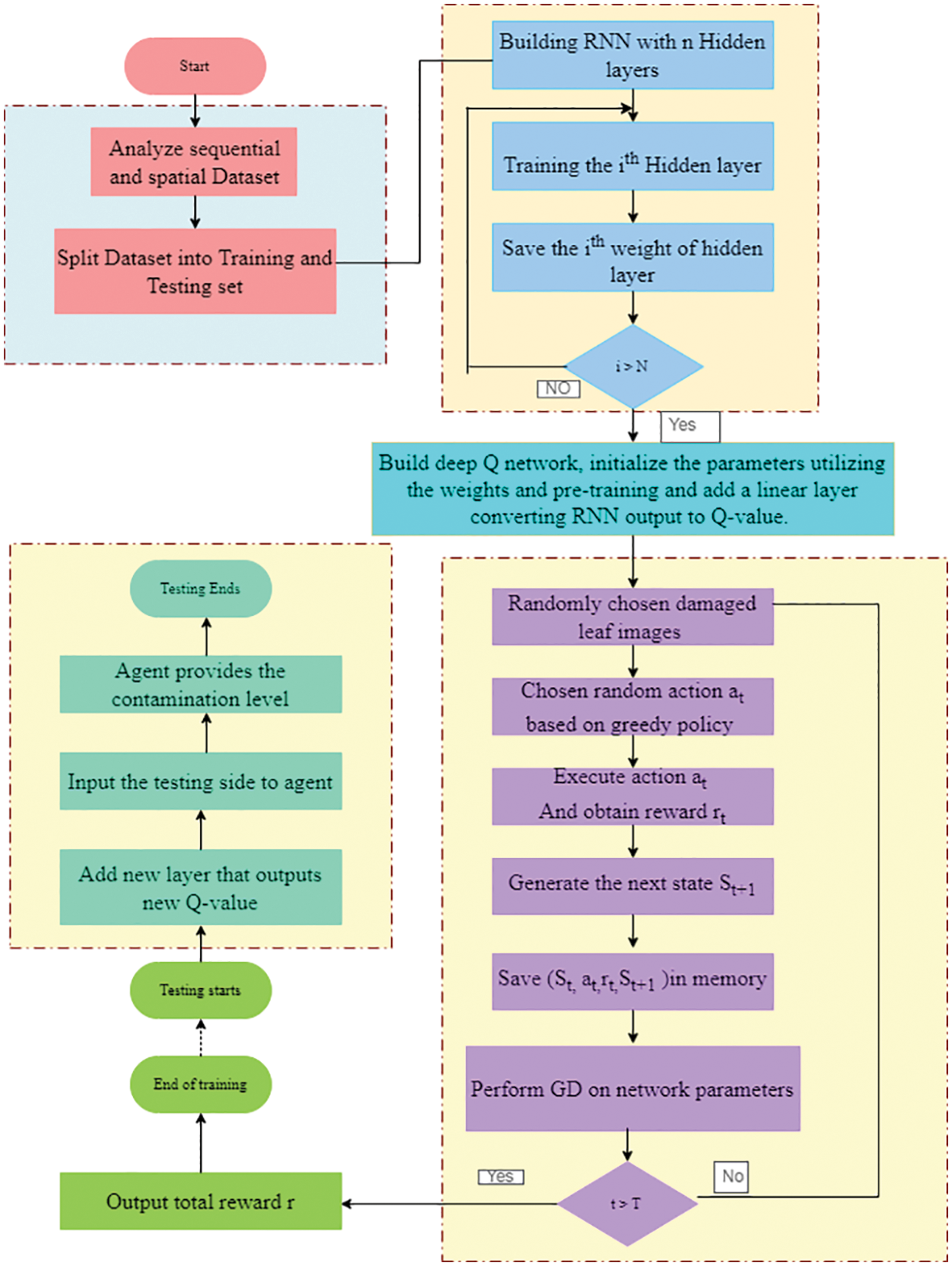
Figure 6: Flow diagram of training RNN

3.3 Decision Making for the Harmfulness of Pesticide Residue Level by Complex Event Processing

Complex event processing (CEP) is indeed an adaptive data processing methodology that originated there in the database area. Any modification in a single data condition is viewed as just an event, as well as the emergence of challenging situations can be seen as the incidence of complex events. This detects complex events through matching the occurrence of such a significant number of events utilizing specific complex event patterns including logical calculations that trigger subsequent actions. CEP technique can completely utilize data from numerous sources to conclude a specific situation. It has excellent asynchronous decoupling and scenario analysis capabilities and is a critical method of real-time processing and automation. This research employed CEP for smart pesticide control there in the agro product ecosystem that created an intelligent pesticide control scheme. This work focuses on the intelligent regulation of pesticide contamination levels in agricultural goods, examines the information generating function and transmission features, and summarises the primary information in a pesticide-free environment.

We propose a novel framework for complex event processing systems that would be appropriate in terms of pesticide contamination levels by examining the similarities and differences of different agricultural challenges. It is critical to encourage the widespread adoption of CEP technology in agriculture and also we developed an automata event accumulation approach, which now allows CEP technology to work more adaptively in complex pesticide control schemes. To determine whether or not high-level complex events occurred, it is essential to examine the logical relationship in time as well as space between low-level basic incidents. This sophisticated event flow is instead generated by calculating the relevant information from high-level events. This process of basic event flow evolving into sophisticated event flow is referred to as event aggregation. This logic which has been formed between events is referred to as event mode. This event processing agent is indeed the unit that performs event pattern matching as well as event creation. Complex events are eventually formed by layer-by-layer aggregation. These occurrences can cause control orders to be issued, additional useful judgment information to be obtained, and the reasoning process to be completed.

The purpose was to evaluate the level of pesticide to be applied in farming on vegetables, fruits, and soil, and the pesticide residues were presented in the output of RNN based on the matching results. By achieving these data, the level is assessed by creating an event comparable to that of CEP, relating to the similarity of two sequences of events. This refers to the measured episodic similarity value, where one is the outcome of matching and the other is the pesticide threshold level. Measurement of this similarity can be given as,

Sim(E1,E2)=semsim(E1,E2)∗semsim(E2,E1) (3)

where E1 and E2 is the episodes that area sequence of events for predicted output and threshold values. Here in (3), semsim(E1,E2) is the similarity between episodes E1andE2 with respect to E2 , likewise semsim(E2,E1) is the similarity between episodes E1andE2 with respect to E1 . Then this Sim(E1,E2) value has been considered for its limit of residue level. The method is then repeated until convergence or the maximum number of iterations is achieved. Thus HCMF finally decides on the pesticide level of contamination.

4  Result and Discussion

This part depicts the simulation result of the proposed framework, which offers a clear concept to test the model’s correctness. This work was completed using the PYTHON working platform with the following system specifications: Windows 8 OS, Intel Core i5 CPU, and 8GB RAM. The proposed HCMF uses three datasets, which are pre-processed and labeled before being sent to CEP for prediction, pattern matching, and decision making based on event production.

CEP obtained the assistance of RNN for pattern matching and discovering similarity scores at this step, and these events are created to decide on the degree of pesticide to be employed in farming. The implementation was carried out in the Python environment, and the performance was evaluated. When examining soil, veggies, including fruits, warmth, moisture, precipitation, kind of soil, category of the crop, phosphorus, nitrogen, potassium as well as nitrate were all taken into account. Those parameters were examined as well as compared to prior techniques including AlexNet [28], BPNN [29], scale-invariant feature transformation (SIFT) [30], PNN [31], and VGGNet [32] in regards to efficiency, predictions, but also processing time.

4.1 Dataset Description

This research took three datasets into account. Each dataset was examined for pesticide contamination levels and the potential harm they may cause to vegetables and fruits. The descriptions of the datasets are provided below.

We are delighted to notify you that around 50,000 expertly curated photographs of healthy as well as sick agro-based plant leaves have become available via the present Kaggle site Plant Village. It was described in the data as well as the platform. It includes apple, blueberry, cherry, maize, peach, orange, potato, and raspberry leaf pictures. After that, the dataset was transformed into a greyscale picture and segmented for further processing.

The second dataset is about soil pollution and the values that come from it. This dataset contains an item for drought level, which was monitored for 90 days using 18 indicators at a specified point in time. Latitude, longitude, median elevation, and slopes are all tabulated values.

The third collection is CSV data for fertilizer prediction. This dataset tracked warmth, moisture, humidity, kind of soil, category of the crop, potassium, phosphorus, and nitrogen as well as nitrate levels. In the suggested model, all three datasets were examined for further processing.

To merge the three datasets, we must first transform the picture dataset to a CSV file by using label binarzior. Now, all the 3 datasets are in the form of CSV file. Then, from the above 3 datasets Nitrogen, Phosphorous, and Potassium values were alone extracted to determine the contamination level in Agri items.

4.2 Performance Evaluation of HCMF

HCMF model has been executed and evaluated for the resultant output. Results are then plotted in the graph for persuasion. Measurement results of humidity, temperature, moisture, nitrogen, phosphorous, potassium, and nitrogen have been given in this section. A contamination level of vegetables, fruits, and soil has been given. Overall performance has been measured and presented to show the efficiency of HCMF.

By analysing the given dataset for a humidity level of prediction the obtained values are plotted as shown in Fig. 7. It shows that humidity values vary with respect to the standard deviation perspective as it was meant to be outliers for the measurement. Humidity values when plotted with respect to fertilizers shows that it remains high in the range of 54–64 for urea, similarly, for Di-ammonium Phosphate (DAP) it remains high at 58–67.5, 14–35–14 fertilizer shows a value of 59–65 as a maximum result, similarly, other fertilizers like 28–28, 17–17–17, 20–20 and 10–26–26 has generated maximum value in the range of 51–62, 53–59 and 54–62.5 respectively.

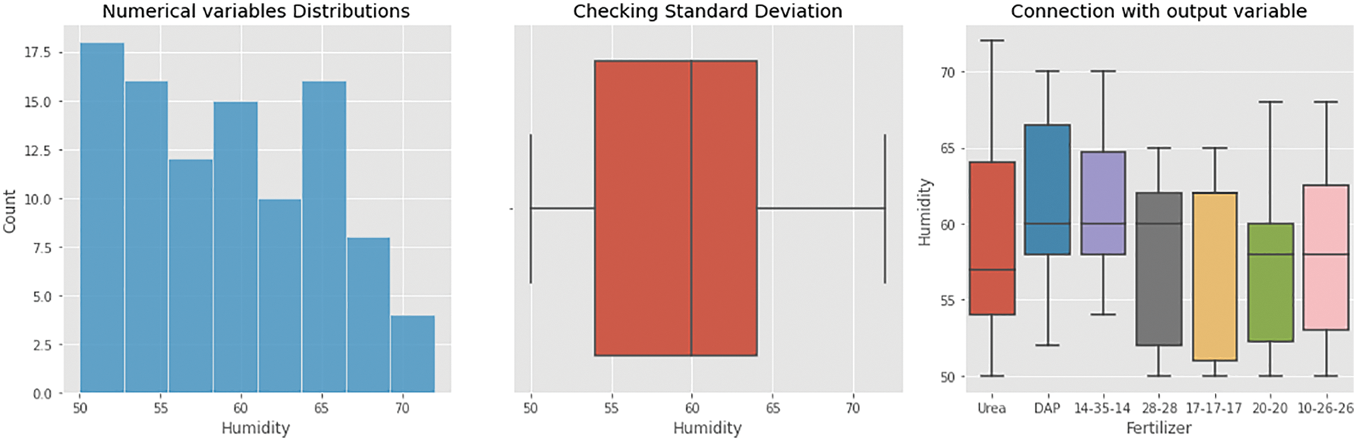
Figure 7: Humidity analysis for the given dataset

The resulting values are displayed in Fig. 8 after analysing the supplied dataset for moisture level prediction. It demonstrates that moisture readings fluctuate depending on the standard deviation, as it was intended to be outliers for the measurement. Moisture values plotted against fertilizers show that urea remains high in the 35–49 range, while DAP remains high at 34–50. The 14–35–14 fertilizer produces a maximum value of 35–47.5, while other fertilizers such as 28–28, 17–17–17, 20–20, and 10–26–26 produce maximum values in the 40–45, 42–55, 36–57, and 36–56 ranges, respectively.

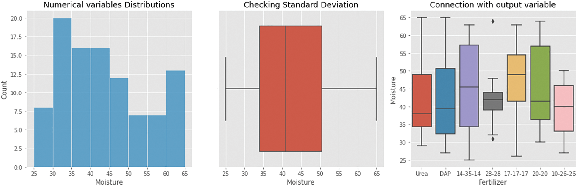
Figure 8: Moisture analysis of an obtained dataset

From Figs. 9–11, analyses of nitrogen, potassium, and phosphorous were made and the results were plotted. Nitrogen analysis of hybrid chronical architecture shows that the fertilizers such as urea, DAP, 14–35–14, 28–28, 17–17–17, 20–20, and 10–26–26 results with the maximum value in certain ranges as that were shown, similarly measuring nitrogen value concerning the numerical distribution has been shown as blue color indicates that the count increases for 10–15 ranges, similarly from Fig. 10, phosphorous as measured with numerical variable distributions has given high value in the range of 0-10 and its SD stands to be high at 10–30 range. Phosphorous study of hybrid chronical architecture reveals that urea, DAP, 14–35–14, 28–28, 17–17–17, 20–20, and 10–26–26 produce the highest value in specific ranges such as 0, 36–40, 28–31, 19–22, 11–17, 10–17 and 18–20 respectively. Potassium analysis was done and the results are plotted in Fig. 11, potassium measured high in the range of 0.0–2.5, the outliers are measured high at 0.0–7.5, Urea, DAP, 14–35–14, 28–28, 17–17–17, 20–20, and 10–26–26 produce the best value in certain ranges, according to potassium research on hybrid chronical architecture.

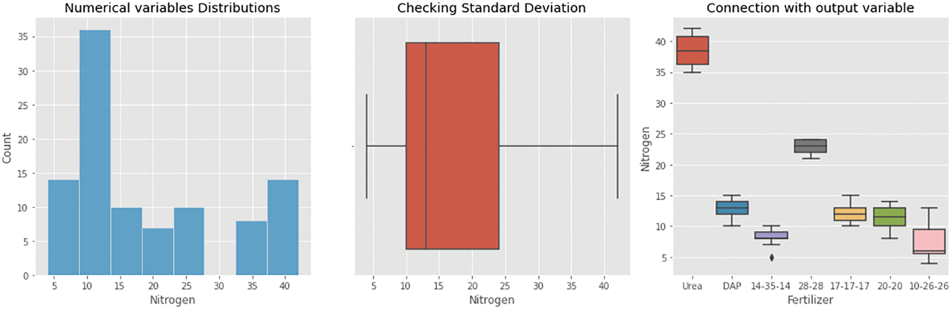
Figure 9: Nitrogen analysis of an obtained dataset

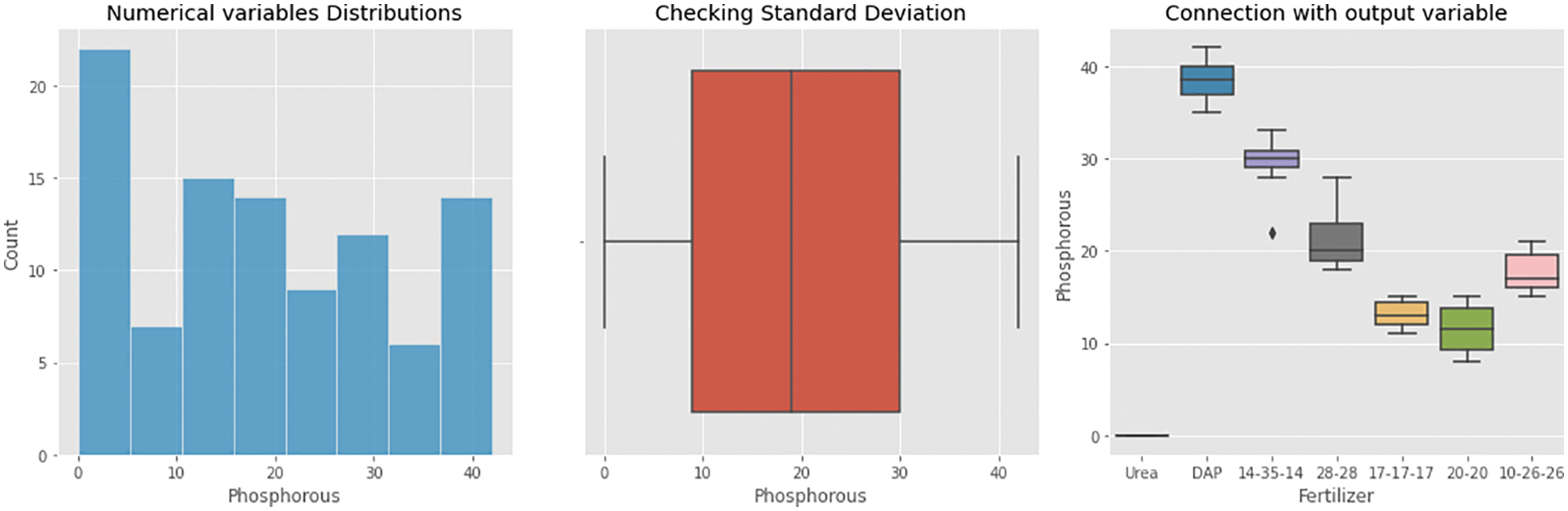
Figure 10: Phosphorous analysis of an obtained dataset

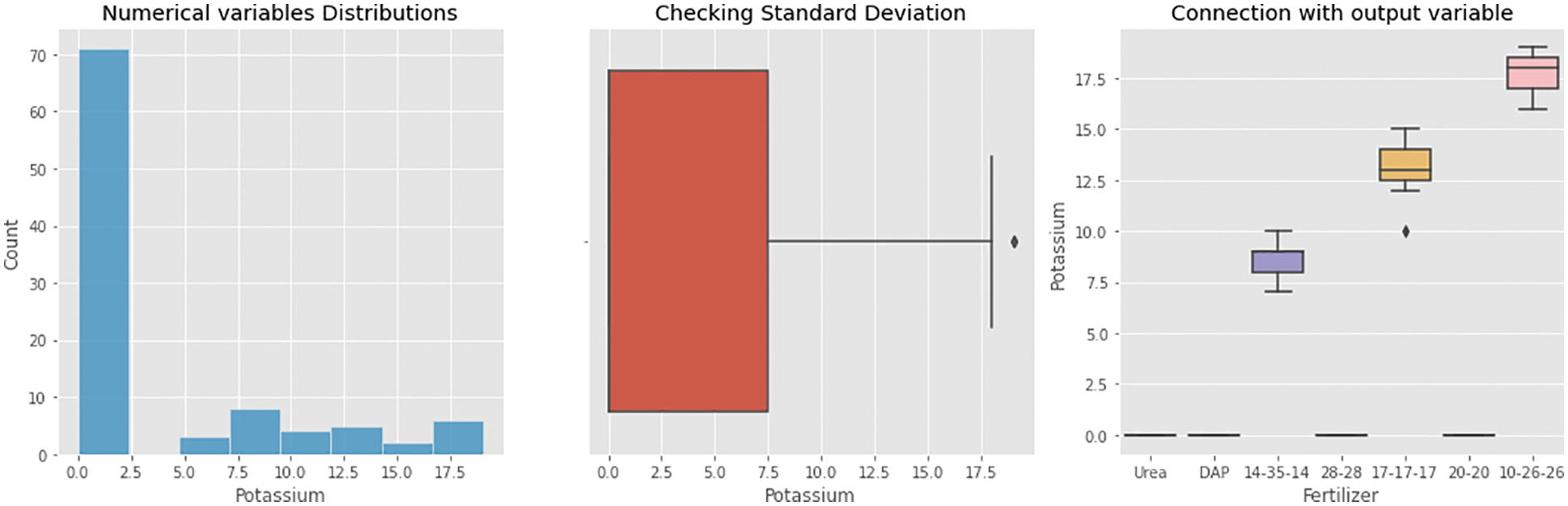
Figure 11: Potassium analysis of an obtained dataset

The resultant values are presented in Fig. 12 after analysing the given dataset for temperature level prediction. It demonstrates that temperature levels fluctuate depending on the standard deviation, as it was intended to be outliers for the measurement. Temperature values plotted against fertilizers show that urea remains high in the 28–33 range, while DAP remains high at 29–35. The 14–35–14 fertilizer produces a maximum value of 29–34, while other fertilizers such as 28–28, 17–17–17, 20–20, and 10–26–26 produce maximum values in the 26–32, 25–30, and 27–32 ranges, respectively.

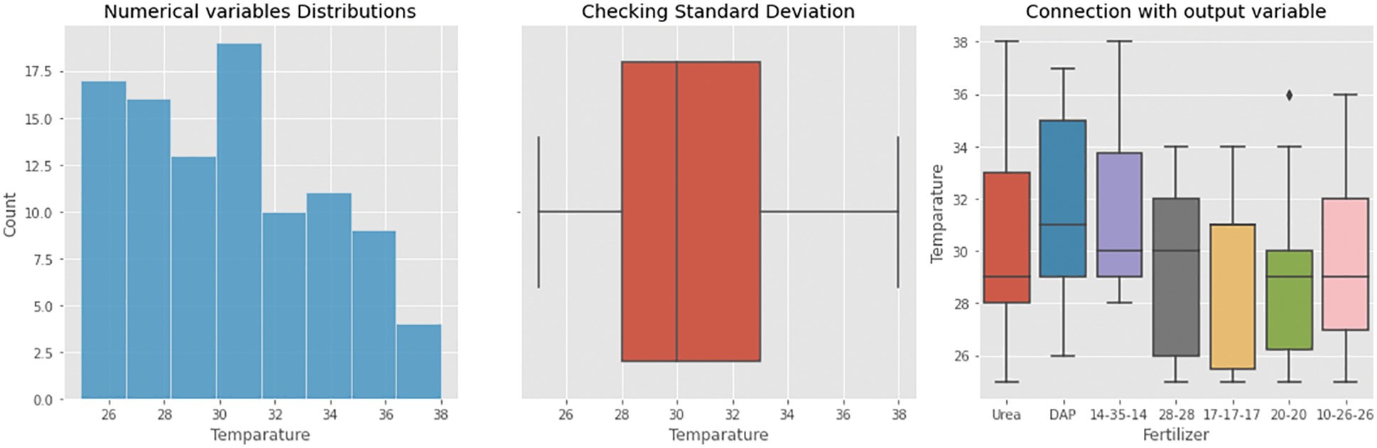
Figure 12: Temperature analysis of an obtained dataset

Measurement of contamination level was done through chemical molecular structure pattern matching via rule policy that was implemented as a CEP framework. Contamination levels are measured for fruits such as apple, strawberry, kiwi, papaya, banana, tomato, spinach, potato, onion, carrot, capsicum, brinjal, radish, and sweet potato as shown in Fig. 13. The values are measured by taking harvested area in the y-axis and contamination level count in the x-axis. This measurement was done by considering nitrogen, phosphorous, and potash as fertilizers for residue measurement. Contamination level measurement was done using HCMF, which was done for both sequential and spatial values as it was the novelist system that can be applied to real-time applications. Similarly, Fig. 14 represents the contamination level in the soil. From the figure, understandably, black soil shows a high contamination level in the range of 27–34, clayey soil shows the next level of contamination in the range of 27–33. Likewise, sandy, loamy and red soil shows its contamination level.

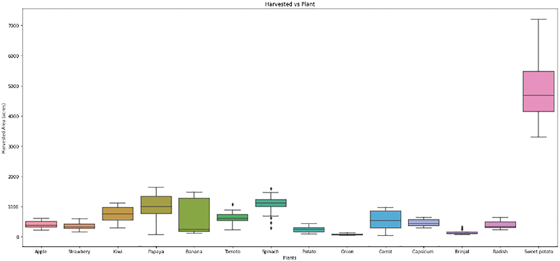
Figure 13: Contamination level measurement in vegetables and fruits

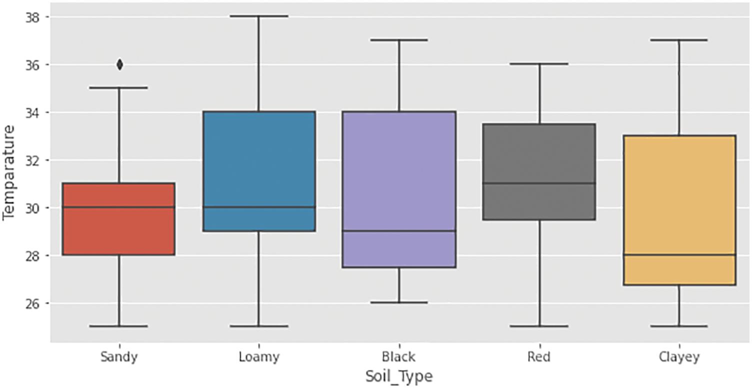
Figure 14: Contamination level measurement in soils

Fig. 15 shows the probability density charts of the given data individually, the suggested approach, and alternative ML algorithms that have been tested. In comparison to the other assessed machine learning strategies, the proposed deep Q learning system can preserve the allocation properties of the realistic agricultural output data more precisely, as shown in Fig. 15. All the measurements were done as pounds/ace value, nitrogen has been found with high-density levels, phosphorous shows density levels of violated values as per threshold stated. The dark red line stated the threshold level and the contamination below them are considered as a healthy level of fertilizer permission and more than that was considered to be non-healthy.

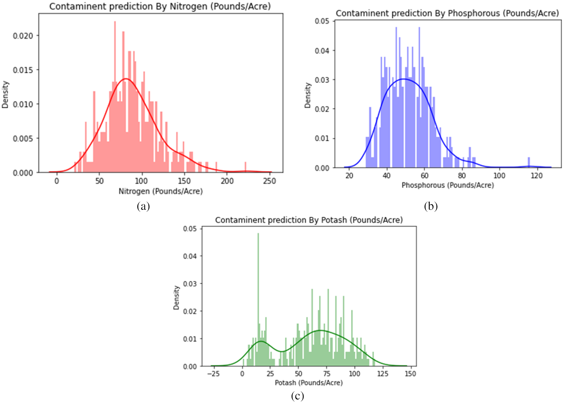
Figure 15: (a) Graphical representation of nitrogen compound contamination level, (b). Graphical representation of Phosphorous compound contamination level, (c). Graphical representation of potash compound contamination level

Fig. 16, shows the contamination level has been made fit concerning the event generated at the end stage of the HCMF result. NPK represents nitrogen, phosphorous, and potassium levels of pesticide contamination in Agri products. After the execution of HCMF, the level has been made fit to the raw values of the pesticide thus making it efficient for real-time applications.

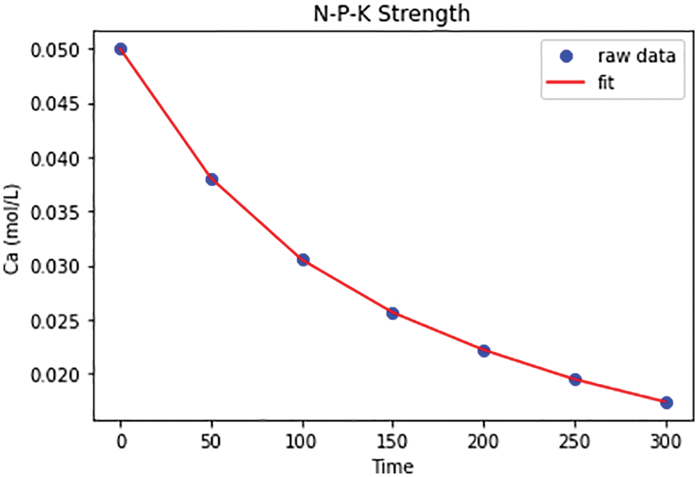
Figure 16: N-P-K strength analysis result

RNN spontaneously learns given data samples, which would be an inherent feature. It’s indeed simple to train individual versions of the algorithm that function well on a specific sort of data. After each action is observed, algorithms that execute sophisticated event recognition should be able to provide incremental forecasts, thereby providing early predictions. Memory episodes are specific examples of more generic complicated occurrences in the world, and they can give important data for mining algorithms that abstract away different event kinds or linkages to construct complex event patterns that were shown in Figs. 17a–17c.

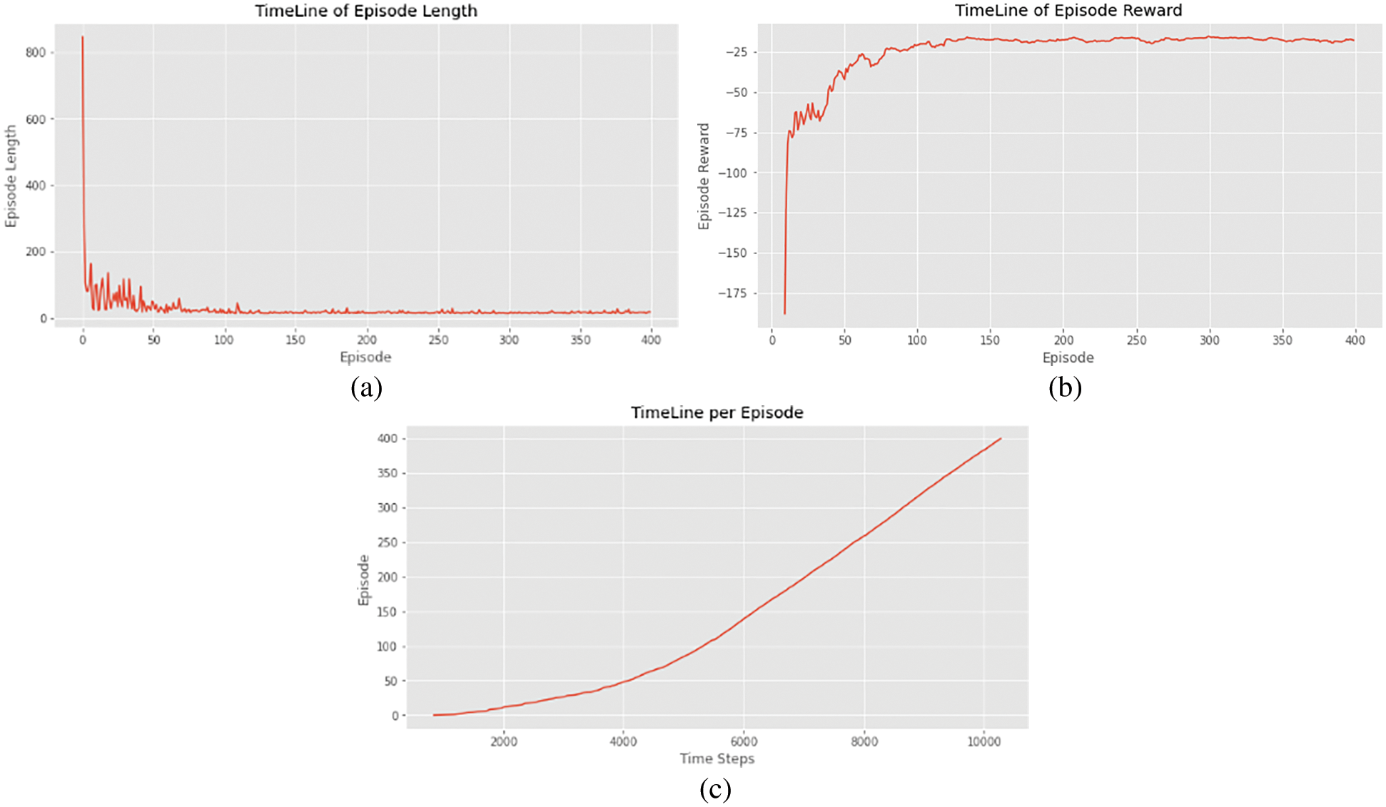
Figure 17: (a) Graphical representation of RNN training timeline of episode length, (b). Graphical representation of episode reward concerning time stamp, (c). Graphical representation of time taken per episode

This ROC curve is indeed a depiction of the rate of false-positive (x-axis) vs the rate of true positive (y-axis) for different available threshold values ranging from 0.0 to 1.0. A true positive rate is typically obtained by dividing the count of true positives by its total of true positives but also false negatives. This reflects how well the model predicts the positive class only when results are good. ROC curve was then shown in Fig. 18, which remains with a high true positive rate shows the efficiency of the RNN model.

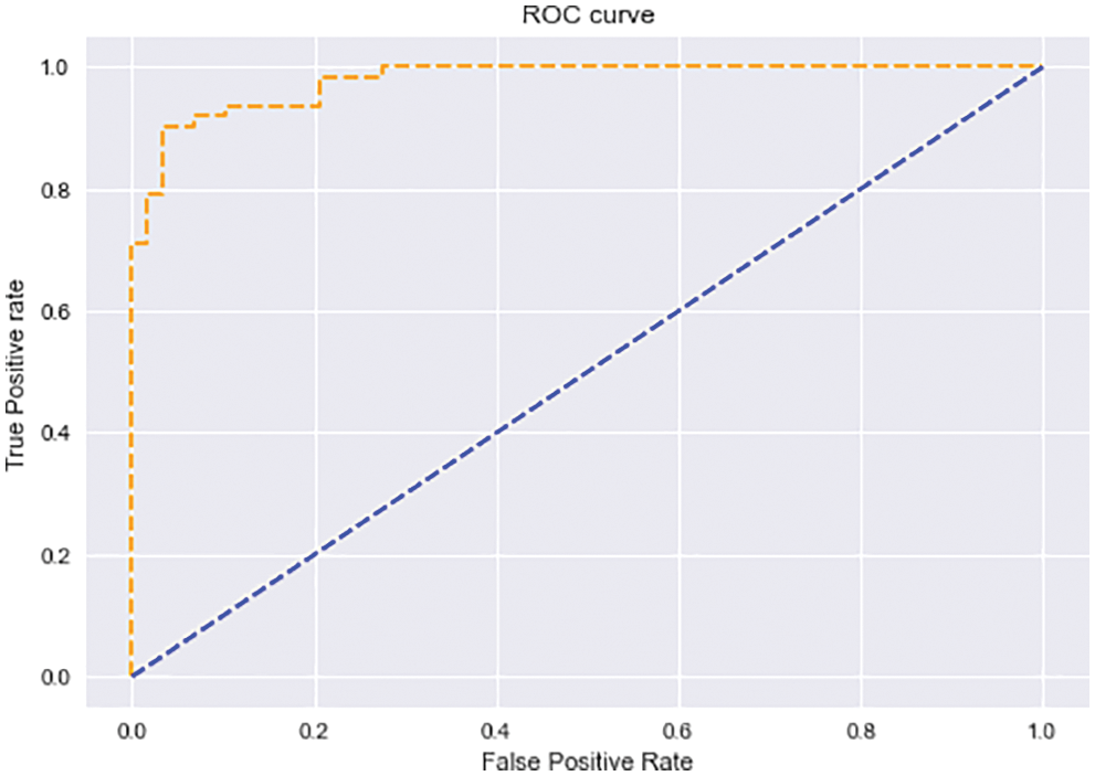
Figure 18: ROC curve for Q learning-based RNN

Figs. 19 and 20 represents the training level accuracy of RNN. Training accuracy was found to be 98.7% has been obtained. Training loss has been measured that was shown to be in the range of 0.30–0.01 values that show that the RNN model has been properly applicable for the real-time application of overall pesticide contamination prediction in the vegetables and fruits values. The performance evaluation of HCMF shows that it has been more efficient and fast throughout the complete implementation process thus making it superior to other pesticide contamination level measurement models. A comparison of HCMF to other existing models has been presented in the next section.

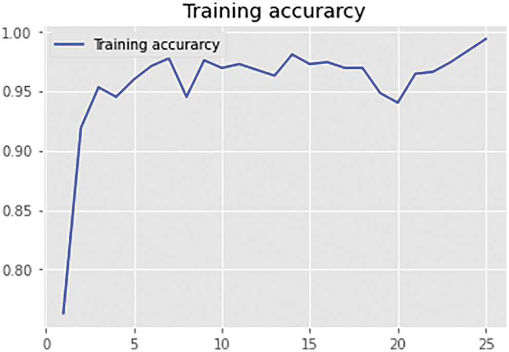
Figure 19: Training accuracy curve for Q learning-based RNN

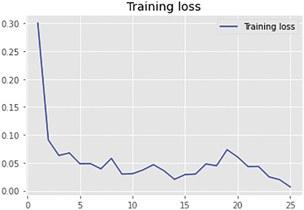
Figure 20: Training loss curve for Q learning-based RNN

4.3 Comparison Analysis of HCMF

Performance matrices that are considered for comparative analysis are defined below

Accuracy- It's level of proximity in assessments of a quantity with vs its actual value is usually defined as just a system’s accuracy.

Prediction level- This is defined as the level of pesticide in the given sample of data and its value is measured concerning the number of samples.

Processing time- Overall processing duration is described as the quantity of time required to analyse the incoming event flow plus interpret that stream of data. The processing time unit is indeed the second.

The graph, as shown in Fig. 21, shows that the proposed model worked well enough to provide high accuracy of 98.7%. Other approaches, such as AlexNet, VGGNet, and BPNN, achieved accuracy levels of 94%, 92%, and 90%, respectively. This accuracy was not up to par; hence the achieved accuracy was lower than that of the proposed model. The accuracy of PNN and SIFT has been reduced to a bare minimum of 88% and 82%, respectively. As a result, the whole proposed model performed well in terms of accuracy, owing to the Q-based learning of RNN, which performs with extremely great accuracy and so improves the proposed framework

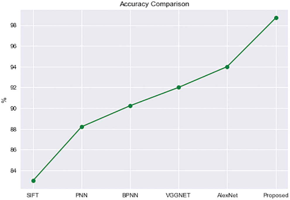
Figure 21: Comparison graph of Accuracy with previous ones

Fig. 22 shows that the proposed model succeeds in terms of prediction accuracy of up to 97 percent. Other approaches, such as AlexNet, have a prediction rate of 93 percent, VGGNet has a prediction rate of 91 percent, BPNN has a prediction rate of 89 percent, and PNN has a prediction rate of 87 percent. SIFT obtained a lower prediction level with an 86 percent prediction value. As a result, the proposed model was obtained with a high prediction value. This was owing to the CEP framework, which applies the prediction level with high predictions, and then rule-based assessment assisted in achieving a high prediction value.

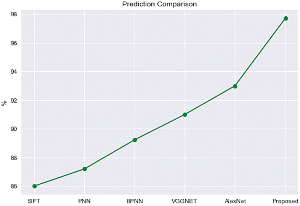
Figure 22: Prediction level comparison graph

The processing time is the time it takes for the entire model to be performed and the outcome to be produced. According to the graph in Fig. 23, the proposed model completes the entire process in 2.5 s, whereas other strategies such as online SVM and CEP take 4.2 s, the RF and CEP scheme takes 6.1 s, and AlexNet takes 7.5 s. HCMF’s processing time was reduced since it used a highly dependable CEP framework that produces speedy results at the application end.

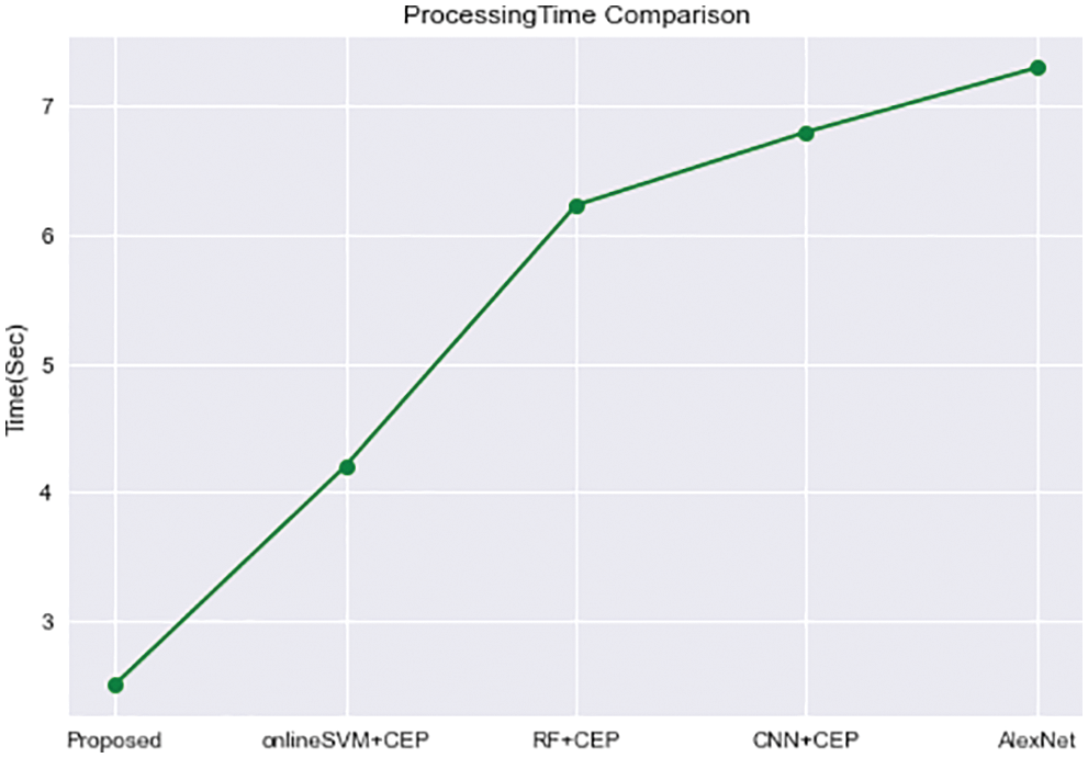
Figure 23: Processing time level comparison

Overall, the examination of the results demonstrates that, when compared to other methodologies, the proposed hybrid chronical architecture is unquestionably the best, with excellent accuracy and little training loss. Following successful investigations into predicting the percentages of affected residue due to fertilizer using chemical structure-based machine learning models and neural networks, it can be concluded that the hybrid chronical model is the most accurate and sensitive model among pesticide contamination models.

5  Conclusion

An HCMF based on CEP and Q learning is proposed in this research to estimate the contamination level of pesticide residue and then continue to decide on its level of harmfulness. A dataset comprising 50,000 carefully selected photos of healthy and sick leaves of agricultural plants, obtained from the current web platform Plant Village, soil contamination and its resulting values in another dataset, and fertilizer prediction CSV data in a third dataset. These datasets have been preprocessed with label binary. Within the CEP framework, a labelled dataset is predicted for the presence of pesticide, matching is done using RNN and its Q learning, and a decision for the amount of contamination is made based on events created. The proposed framework achieves 98.7 percent accuracy with a training loss of 30%, according to the results. To fully understand pesticide utilization or even management throughout the future, more research will be conducted on both occupational and ecologic exposures, as well as the associated health hazard evaluation of pesticides. Furthermore, future research might include integrating the IoT with the CEP framework to monitor pesticides and make further decisions.

Acknowledgement: The authors wish to thank the Department of Computer Science and Engineering, KPR Institute of Engineering and Technology, to provide the computing facilities for project execution.

Funding Statement: The authors received no specific funding for this study.

Conflicts of Interest: The authors declare that they have no conflicts of interest to report regarding the present study.

References

 1.  D. W. Park, Y. S. Yang, Y. U. Lee, S. J. Han, H. J. Kim et al., “Pesticide residues and risk assessment from monitoring programs in the largest production area of leafy vegetables in South Korea: A 15-year study,” Foods, vol. 10, no. 2, pp. 425, 2021. [Google Scholar]

 2.  C. Pelosi, C. Bertrand, G. Daniele, M. Coeurdassier, P. Benoit et al., “Residues of currently used pesticides in soils and earthworms: A silent threat,” Agriculture Ecosystems & Environment, vol. 305, no. 10, pp. 107167, 2021. [Google Scholar]

 3.  A. Schecter, J. Colacino, D. Haffner, K. Patel, M. Opel et al., “Per fluorinated compounds, polychlorinated biphenyls, and organochlorine pesticide contamination in composite food samples from Dallas, Texas, USA,” Environmental Health Perspectives, vol. 118, no. 6, pp. 796–802, 2010. [Google Scholar]

 4.  A. K. Richardson, M. Chadha, H. Rapp-Wright, G. A. Mills, G. R. Fones et al., “Rapid direct analysis of river water and machine learning assisted suspect screening of emerging contaminants in passive sampler extracts,” Analytical Methods, vol. 13, no. 5, pp. 595–606, 2021. [Google Scholar]

 5.  J. Wei, X. Wang, Z. Wang and J. Cao, “Qualitative detection of pesticide residues using mass spectral data based on convolutional neural network,” SN Applied Sciences, vol. 3, no. 7, pp. 1–13, 2021. [Google Scholar]

 6.  N. Mehdiyev, J. Krumeich, D. Enke, D. Werth and P. Loos, “Determination of rule patterns in complex event processing using machine learning techniques,” Procedia Computer Science, vol. 61, no. 8, pp. 395–401, 2015. [Google Scholar]

 7.  D. Elavarasan and P. D. Vincent, “Crop yield prediction using deep Q learning model for sustainable agrarian applications,” IEEE Access, vol. 8, pp. 86886–86901, 2020. [Google Scholar]

 8.  Y. Jia and X. Li, “Complex event processing methods for greenhouse control,” Agriculture, vol. 11, no. 9, pp. 811, 2021. [Google Scholar]

 9.  N. Mehdiyev, J. Krumeich, D. Enke, D. Werth and P. Loos, “Determination of rule patterns in complex event processing using machine learning techniques,” Procedia Computer Science, vol. 61, no. 8, pp. 395–401, 2015. [Google Scholar]

10. A. Ramírez, N. Moreno and A. Vallecillo, “Rule-based pre-processing for data stream mining using complex event processing,” Expert Systems, vol. 38, no. 8, pp. e12762, 2021. [Google Scholar]

11. E. Alevizos, A. Artikis and G. Paliouras, “Complex event forecasting with prediction suffix trees,” The VLDB Journal, vol. 31, no. 1, pp. 1–24, 2021. [Google Scholar]

12. K. Zhang, Z. Yang and T. Başar, “Multi-agent reinforcement learning: A selective overview of theories and algorithms,” Handbook of Reinforcement Learning and Control, vol. 325, pp. 321–384, 2021. [Google Scholar]

13. R. Bhargavi, “Complex event processing framework for big data applications,” in Data Science and Big Data Computing. Cham: Springer, pp. 41–56, 2016. [Google Scholar]

14. T. Lykouris, M. Simchowitz, A. Slivkins and W. Sun, “Corruption-robust exploration in episodic Q learning,” in Conf. on Learning Theory, PMLR, New York, pp. 3242–3245, 2021, July. [Google Scholar]

15. M. H. EL-Saeid and A. G. Alghamdi, “Identification of pesticide residues and prediction of their fate in agricultural soil,” Water Air, & Soil Pollution, vol. 231, no. 6, pp. 1–10, 2020. [Google Scholar]

16. D. Devi, A. Anand, S. S. Sophia, M. Karpagam and S. Maheswari, “IoT-deep learning based prediction of amount of pesticides and diseases in fruits,” in 2020 Int. Conf. on Smart Electronics and Communication (ICOSECTrichy, India, IEEE, pp. 848–853, 2020. [Google Scholar]

17. E. Malaj, K. Liber and C. A. Morrissey, “Spatial distribution of agricultural pesticide use and predicted wetland exposure in the Canadian Prairie Pothole Region,” Science of the Total Environment, vol. 718, pp. 134765, 2020. [Google Scholar]

18. L. Chavez Rodriguez, B. Ingalls, E. Schwarz, T. Streck, M. Uksa et al., “Gene-centric model approaches for accurate prediction of pesticide biodegradation in soils,” Environmental Science & Technology, vol. 54, no. 21, pp. 13638–13650, 2020. [Google Scholar]

19. V. Silva, X. Yang, L. Fleskens, C. Ritsema and V. Geissen, “Soil contamination by pesticide residues-What and how much should we expect to find in EU agricultural soils based on pesticide recommended uses,” in EGU General Assembly Conf. Abstracts, held online 4–8 May, 2020, pp. 16476, 2020. [Google Scholar]

20. D. G. DiGiacopo and J. Hua, “Evaluating the fitness consequences of plasticity in tolerance to pesticides,” Ecology and Evolution, vol. 10, no. 10, pp. 4448–4456, 2020. [Google Scholar]

21. X. Tang, W. Xiao, T. Shang, S. Zhang, X. Han et al., “An electronic nose technology to quantify pyrethroid pesticide contamination in tea,” Chemosensors, vol. 8, no. 2, pp. 30, 2020. [Google Scholar]

22. G. Bhandari, K. Atreya, P. T. Scheepers and V. Geissen, “Concentration and distribution of pesticide residues in soil: Non-dietary human health risk assessment,” Chemosphere, vol. 253, no. 2, pp. 126594, 2020. [Google Scholar]

23. G. K. Blankson, P. Osei-Fosu, E. A. Adeendze and D. Ashie, “Contamination levels of organophosphorus and synthetic pyrethroid pesticides in vegetables marketed in Accra,” Ghana Food control, vol. 68, no. 6, pp. 174–180, 2016. [Google Scholar]

24. G. Allen, C. J. Halsall, J. Ukpebor, N. D. Paul, G. Ridall et al., “Increased occurrence of pesticide residues on crops grown in protected environments compared to crops grown in open field conditions,” Chemosphere, vol. 119, pp. 1428–1435, 2015. [Google Scholar]

25. Y. Zhu, M. Li, D. Yu and L. Yang, “A novel paper rag as ‘D-SERS’ substrate for detection of pesticide residues at various peels,” Talanta, vol. 128, no. 1, pp. 117–124, 2014. [Google Scholar]

26. M. U. Madhav, D. N. Jyothi and P. Kalyani, “Prediction of pesticides and identification of diseases in fruits using Support Vector Machine (SVM) and IoT,” in AIP Conf. Proc., AIP Publishing LLC, Surabaya, Indonesia, vol. 2407, pp. 20016, 2021. [Google Scholar]

27. https://towardsdatascience.com/deep-q-network-combining-deep-reinforcement-learning-a5616bcfc207. [Google Scholar]

28. B. Jiang, J. He, S. Yang, H. Fu, T. Li et al., “Fusion of machine vision technology and AlexNet-CNNs deep learning network for the detection of postharvest apple pesticide residues,” Artificial Intelligence in Agriculture, vol. 1, no. 1, pp. 1–8, 2019. [Google Scholar]

29. S. Sladojevic, M. Arsenovic, A. Anderla, D. Culibrk and D. Stefanovic, “Deep neural networks based recognition of plant diseases by leaf image classification,” Computational Intelligence and Neuroscience, vol. 2016, no. 6, pp. 1–11, 2016. [Google Scholar]

30. J. Alamri, R. Harrabi and S. B. Chaabane, “Face recognition based on convolution neural network and scale invariant feature transform,” International Journal of Advanced Computer Science and Applications(IJACSA), vol. 12, no. 2, pp. 644–654, 2021. [Google Scholar]

31. H. M. Afify, K. K. Mohammed and A. E. Hassanien, “Multi-images recognition of breast cancer histopathological via probabilistic neural network approach,” Journal of System and Management Sciences, vol. 1, no. 2, pp. 53–68, 2020. [Google Scholar]

32. B. S. Rao, “Accurate leukocoria predictor based on deep VGG-net CNN technique,” IET Image Processing, vol. 14, no. 10, pp. 2241–2248, 2020. [Google Scholar]