Machine Learning-based Inverse Model for Few-Mode Fiber Designs

1  Introduction

The backbone network traffic is growing at a rate of ten times every five years. With data rates of many gigabits per second, optical fibers are the most efficient media for handling recent network traffic. For existing wireless backhaul networks, these are preferred over other mediums of communication. Optical fibers are now favored for frontend networks to connect dense meshes of 5G cells due to their huge bandwidth. Fibers are less resistant to electromagnetic interference and have a low attenuation rate, allowing them to manage high data rates. Fibers also provide the most secure mode of communication. In the previous three decades, optical fiber transmission capacity has increased by a factor of five, thanks to these advantages [1].

To handle the network traffic in recent years different types of fibers have been designed and developed as multi-mode fiber (MMF), single-mode fiber (SMF), and its variants like step-index fiber (SIF), graded-index fiber (GIF) [2]. However, the theoretical transmission capacity of SMFs is limited to 100 Tbps under limited transmissible power through the core [3] and nonlinear effects [4]. Hence, some special fibers namely few-mode fibers (FMFs) [5], multi-core fibers (MCFs) [6], polarization-maintaining weakly coupled FMF [7], and few-mode multi-core fibers (FM-MCFs) [8] are designed for next-generation communication using mode division multiplexing (MDM) [9] and spatial division multiplexing (SDM) [10]. The MDM transmission is classified as weakly coupled [11] and strongly coupled [12]. The FMF is an excellent candidate for high-speed data communication using weakly coupled MDM [13]. For short-reach MDM and SDM transmission using direct-detection (DD) FMFs are preferable over MCFs [14]. The receiver design complexity using DD is less in weakly coupled MDM links [15]. This motivates us to propose and design weakly coupled FMFs for MDM transmission.

The MDM link’s transmission capacity is proportional to the number of modes passing through the few-mode fibers. As a result, the research community is becoming more interested in the design of FMFs to improve the spectral efficiency of recent optical networks. In [16–29] some recent works on weakly coupled FMFs have been investigated and depicted in Fig. 1. Through this literature, we have mainly investigated two important profiles of FMF, namely, the ring-core profile and the graded-index (GI) profile. Fig. 1, depicts the recent evolutions in the design of weakly coupled FMFs based on the number of linearly polarized (LP) modes over the years. The number of modes through the weakly coupled FMF and the coupling between them is controlled by the refractive index profile (RIP) and the profile parameters of FMF. Managing the number of modes, low mode coupling within the adjacent modes, low differential mode delay (DMD), low dispersion, large effective mode-area (Aeff), and low bending loss are the challenging issues in the design of FMFs. These challenges can be resolved by the proper choice of RIP and the profile parameters of FMFs. The two important characteristics to be considered during the design of weakly coupled FMF design are the number of unique modes supported by the fiber structure and the effective index difference (Δneff) between the modes. For weakly coupled MDM link setup, the min (Δneff) between the adjacent non-degenerate LP mode groups should be greater than 1 × 10−3 (minΔneff≥1×10−3) [23]. The conventional method of designing the FMFs through parametric sweep is time-consuming for a complex structure. To obtain the multiple parameters through simulation in the acceptable range for fabrication is very tedious as well. This motivates us to work on the inverse design of FMFs using ML models.

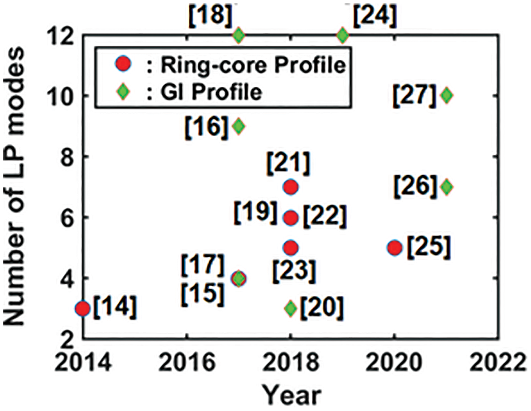
Figure 1: Recent evolutions in the design of weakly coupled ring-core and GI FMFs over the years

To date in the area of optical fiber design particle swarm optimization (PSO) [30], a genetic algorithm (GA) [31] has been demonstrated by the authors. But, these optimization techniques provide less accuracy for complex fiber structures. At the same time, the process is not reusable. In forward design, the profile parameters of an FMF structure change with change in the number of modes and Δneff. Thus the design parameters are fixed and not reusable.

Machine learning is an emerging technology in recent years. This can be used in every field for optimization, prediction, classification, and forecasting. The authors in [32] have proposed a transfer learning based on a convolutional neural network (CNN) to diagnose the COVID-19 patients accurately. He et.al., in [33] have demonstrated ML-based inverse designing of FMF design by using a neural network (NN). In their work, the authors have demonstrated the inverse design for weak coupling optimization in step-index few-mode fiber with 4-rings to guide 4, 6, and 10 modes and also optimize the profile parameters for 6-ring to achieve 20 modes with weak coupling. The ML-based inverse modeling is a highly accurate, fast, and reusable method of few-mode fiber design. We have listed some of the techniques proposed by the authors for application in fiber design in Tab. 1.

This motivates us to further work on inverse modeling for predicting the profile parameters of a ring-core FMF for a specific number of LP modes with optimization of mode coupling (minΔneff≥1×10−3) between the adjacent modes. In this work, we have used regression models in machine learning to predict the profile parameters of weakly coupled ring-core FMF. We have demonstrated the inverse modeling of the proposed FMF with three regression-based ML models such as ordinary least-square linear multiple regressions, k-nearest neighbors of multi-output regression, and decision trees for multi-output regression. And we have found decision tree for multi-output regression is the robust, highly-accurate ML model for fast modeling of FMFs. The use of regression models for predicting multiple profile parameters of complex FMF structures is being done for the first time according to the best of our knowledge. This work can be further extended for different FMF structures and will show possible applications in the fiber modeling industry.

2  Design Process

2.1 Fiber Design

With keeping in mind weak coupling optimization for a specific number of modes under fabrication feasibility we have proposed a ring-core FMF. Various FMF profiles had been proposed over the past years to make the trade-off between weak mode-coupling and low DMD. Among them, graded-index profiles [34], ring-core fiber [16], and multi-core few-mode [35] are the commonly used FMF profiles that support MDM transmission. In one of our recent works [29], we have introduced a gaussian-core FMF with a cladding trench to support ten-LP modes with minΔneff≥1×10−3 , min DMGD ≤ 0.3 ps/m and effective area Aeff in the range of 150–300 µm2 over the C-band. But out of all the FMF profiles, the ring-core fiber structure is similar to that of step-index fiber (SIF). The fiber profile is having a limited number of design parameters. These parameters can be easily optimized to allow a specific number of modes [16,21,24] with weak coupling among the adjacent modes. This motivates us to propose a modified ring-core FMF with three rings. The proposed fiber is designed through inverse modeling followed by ML for a target number of modes with low coupling between the guided modes.

The refractive index profile and crossectional view of the proposed FMF are shown in Figs. 2a and 2b, respectively. The proposed FMF is designed with 3-rings to make the fabrication process less complex as compared to the structure in [33]. The proposed design is assumed with a cladding diameter of 125 µm and the host material of Silica to satisfy the commercially available fibers fabrication technologies. The variation of the refractive index profile of the ring-core as a function of the radial distance is given in Eq. (1). The refractive index of each of the rings is made up and down as that of the cladding. The cladding refractive index is noted as nclad. The refractive indices of the first, second, and third rings are n1, n2, and n3, respectively. The first ring is down-doped as that of the 2nd ring at the same time the 2nd ring is made down as that of the cladding to reduce coupling between higher-order modes. The range of other parameters is so chosen to satisfy the cost-effective fabrication criteria. Ring radius (ri) and refractive index difference between ith ring and cladding (Δi) are the important profile parameters of the proposed FMF. The proposed FMF is assumed with three rings, hence the parameters are noted with i = 1, 2, 3. The set of profile parameters that define the modal characteristics of the proposed FMF is [r1, r2, r3, Δ1, Δ2, Δ3].

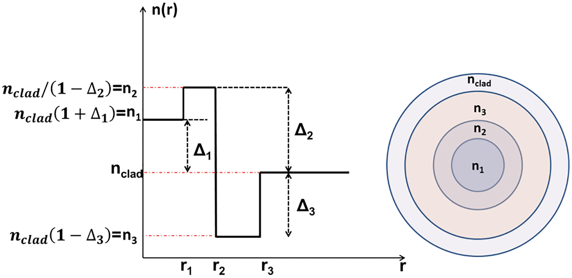
Figure 2: (a) The refractive index profile as a function of radial distance, and (b) cross-sectional view of the proposed ring-core FMF, respectively

nco(r)={n1=nclad(1+Δ1)0≤r≤r1n2=nclad/(1−Δ2)r1≤r≤r2n3=nclad(1−Δ3)r2≤r≤r3 (1)

2.2 Data Set Generation

For ML the first step is to create a suitable data set. The size of the data set for training is very important. Too large data increases the training time and too small data is not suitable for accurate prediction of the required parameters. The parameters of the proposed ring-core FMF in Fig. 2 are varied within an appropriate range to obtain a specific number of modes with weak coupling between a few of the adjacent modes. The parameters [r1, r2, r3, Δ1, Δ2, Δ3] are given as input to the finite element method (FEM) based on commercially available software COMSOL to obtain the mode solutions (neff) for each of the guiding modes. These mode solutions are arranged in a 5000 × 33 matrix for training and testing. One set of data took 30 minutes for generation and compilation. The data set is created by varying the range of design parameters ri and Δi as given in Tab. 2. The range of the design parameters is varied to achieve a maximum 26 number of modes over an extensive range of neff. The range of design parameters is selected to achieve a large number of modes and more than 50% of the mode solutions satisfy the criteria of weak mode coupling (minΔneff≥1×10−3) .

2.3 Machine Learning Process

The entire design process of the proposed FMF is divided into two parts: forward design and inverse modeling. The forward design process is followed to create a data set for the ML models as discussed in Section 2.2. The ML models are used to create a bridge between desired outputs and required structural parameters. Machine learning makes the inverse modeling process fast and highly accurate. After creating the suitable data set it is undergone through min-max normalization and then given as the input to ML models for training. The entire inverse design process using ML models is depicted in Fig. 3. The models are validated by assuming 70% of data for training and 30% for testing. With this ratio, we have achieved the best-predicted results. After validating the accuracy of the ML models the profile parameters are predicted for the desired number of modes by giving targets to the trained models. These predicted parameters are used for inverse modeling of the proposed FMF by giving them as the input to the COMSOL software. The target solutions are then compared with the actual solutions to validate the accuracy of the inverse design process with relative error. The parameters in the proposed model have been selected so that the error between the actual and the predicted value is minimum.

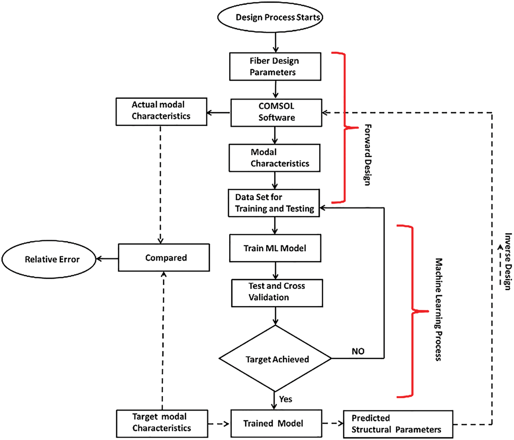
Figure 3: Flow diagram for the regression-based inverse design process for ring-core FMF

2.4 Regression Model

In this work, we have used the regression models as they easily map the secondary target (Δneff) with the structural parameters of the proposed FMF. These models have no fitting problem rather than provide better accuracy with less number of training samples. We use the data set to train and validate the regression-based ML models. These ML models are used to predict the target structural parameters for the inverse design of the proposed FMF. The regression-based ML models are highly accurate and offer fast prediction techniques for a specific number of modes with weak mode coupling. Here, we have demonstrated three different types of regression models, namely, ordinary least-square linear multiple regressions, k-nearest neighbors of multi-output regression, and multivariate ID3-based decision trees for regression.

2.4.1 Ordinary Least-Square Linear Multiple Regressions

This model predicts the multiple targets by linear approximation. The objective of this model is to minimize the residual error between the predicted target and observed data by fitting the predicted target to a linear model with coefficients x=(x1x2…xN) . The model can be represented mathematically as in Eq. (2) [36]. In Eq. (2) Ai is the model output for the ith sample, Bij are the predicted variables that are linearly mapped to the model output, xj is the regression coefficient, and ϵi is the residual error. The error is assumed to be normally distributed. In this wok, we have focused on the multiple linear regressions because the set of the mode solutions (neff) used for training the model are the function of ri and Δi.

Ai=∑j=1N⁡Bijxj+ϵi (2)

2.4.2 k-nearest Neighbors of Multi-Output Regression

The k-nearest neighbor (k-NN) ML algorithm is based on supervised learning. This is the simple non-parametric ML algorithm. During prediction, k-NN finds the similarity between the target and the available data set and creates a cluster of very similar points. The k neighbors of the target have been found by calculating the Euclidean distance d(yi,yj)=∑k=1K⁡[yki−ykj]2 between the data points. The output is predicted by the model when it finds the target belongs to one category which contains the maximum number of neighbors. The predicted output A^ for the k-nearest neighbors of multi-output regression can be expressed as shown in Eq. (3) [37]. In our work, we have used multi-output k-NN because we are predicting six profile parameters of the proposed FMF namely, [r1, r2, r3, Δ1, Δ2, Δ3] by training the ML models.

A^(y)=1k∑yiϵNk(y)⁡Ai (3)

2.4.3 ID3-Based Decision trees for Multi-Output Regression

The decision tree (DT) algorithm is also based on supervised learning. This technique is used for both prediction and classification problems. It uses a binary tree structure to predict the target from a series of binary splits. The decision tree begins with a root node and terminates with the decision leaves. Each DT consists of three types of nodes, root nodes, decision nodes, and leaf nodes. The node from which the decision begins and the population starts is known as the root node. The nodes which are generated after splitting the root node is called decision node. The nodes where a further decision is not possible are called leaf nodes. For this work, the decision tree is made through the modified ID3 algorithm for multivariate input-output prediction. As it is the inverse design this algorithm is suitable due to its working in a top-down approach. The steps involved in the ID3 algorithm are as follows:

The entropy for multiple attributes is calculated by using Eq. (4).

E(CS,SA)=∑x∈SA⁡P(x)E(x) (4)

where CS: current state and SA: selected attributes and E(x) is the entropy of a single attribute E(x)=∑i=1x−pilog2pi , with pi being the probability of a single event [38]. The IG is obtained by Eq. (5).

IG(CS,SA)=E(CS)−E(CS,SA) (5)

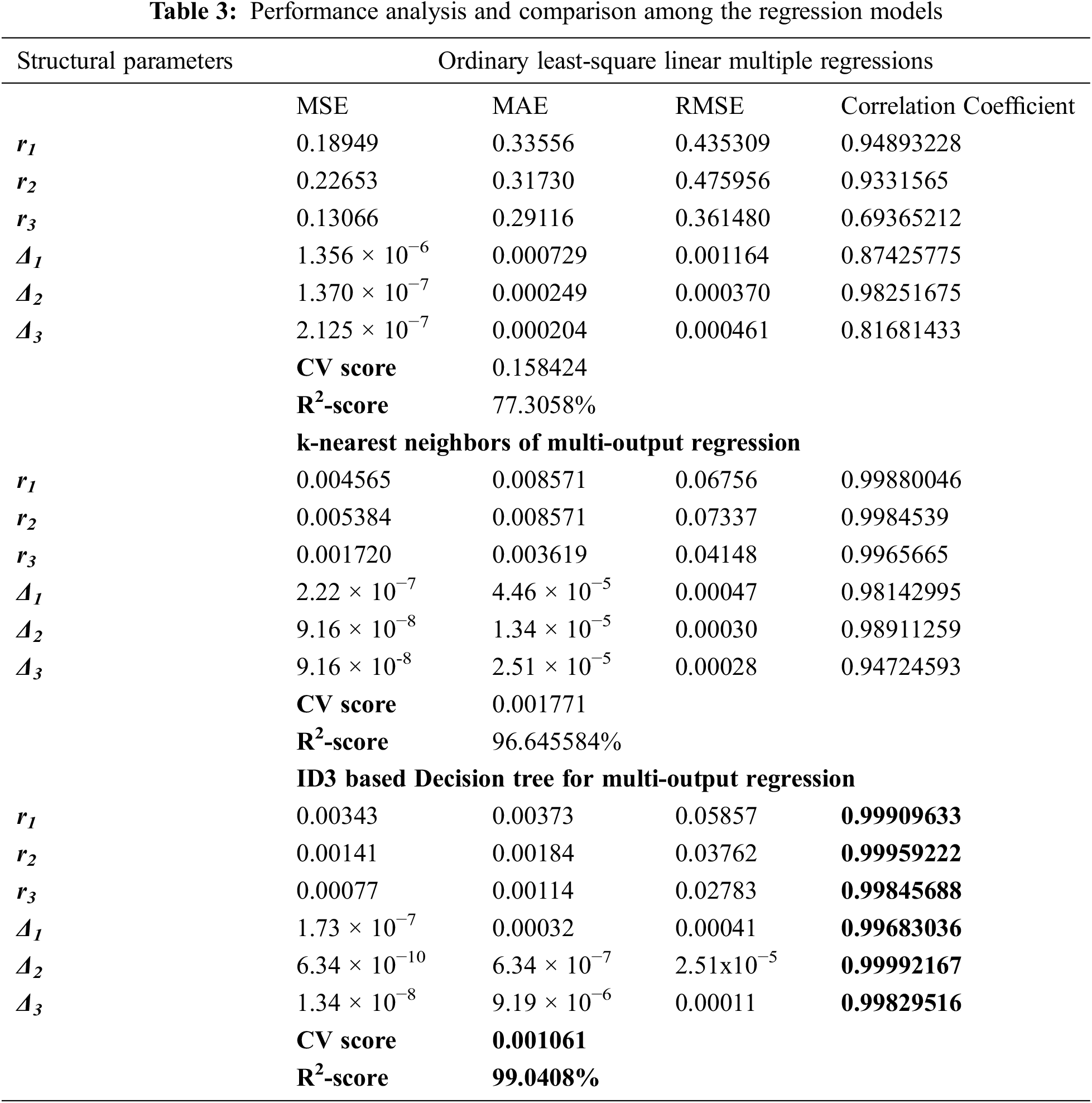
The work is carried out in the open-source python platform. The plots for test and predicted outputs of ordinary least-square linear multiple regressions, k-nearest neighbors of multi-output regression, and ID3-based decision trees for multi-output regression are shown in Figs. 4–6 in the Result Section, respectively. The accuracy and robustness of the models have been determined using ten-fold cross-validation (CV). This technique randomly selects 30% of the data on a rotation basis from the whole data set that is not included in the training data set for validating how accurately the model fits the structural parameters. The CV score is obtained by computing the negative mean absolute error. The model with the lowest CV score is treated as the most robust model. The performance of the models is evaluated by computing the error functions and R2-score. The errors such as mean square error (MSE), mean absolute error (MAE), and root mean squared error (RMSE) is determined for each ML model. The model with the minimum error and maximum R2-score gives the more accurate prediction result. Tab. 3 in the Result Section describes the performance comparison between all three models. We have found ID3-based decision tree for multi-output regression is the most robust, highly-accurate ML model for inverse modeling of FMFs, as is evident from the test and predicted output plots in Figs. 4–6, and from the results in Tab. 3.

Figure 4: The mapping plot between the actual and predicted data using Ordinary Least-square Linear Multiple Regressions for all the structural parameters

Figure 5: The mapping plot between the actual and predicted data using k-nearest Neighbors of Multi-output Regression for all the structural parameters

Figure 6: The mapping plot between the actual and predicted data using ID3-based Decision trees for Multi-output Regression for all the structural parameters

3  Results and Discussion

The above technique is used to predict the structural parameters for the proposed ring-core FMF structure for 5, 10, 15, and 20 modes with weak coupling optimization. The input data set for training are the effective index values for the guided modes and the number of guided modes with their respective profile parameters. For the M-number of modes the training data set is [r1, r2, r3, Δ1, Δ2, Δ3, neff1, neff2, neff3, neff4, ….. neffi,….. neffM, M] where neffi is the effective refractive index of the ith mode solution. The data set is obtained from COMSOL for a specific combination of structural parameters [r1, r2, r3, Δ1, Δ2, Δ3]. If for a combination of the profile parameters the ith mode solution is not obtained, then the corresponding data in the training data set is assigned with zero. For prediction, a target data set [neff1, neff2, neff3, neff4, ….. neffi,….. neffM, M] is created to maintain minΔneff between the adjacent modes. This is given as the input to the trained models. Through prediction, the trained models give the structural parameters [r1, r2, r3, Δ1, Δ2, Δ3] outputs. These predicted outputs are used as input to COMSOL for the inverse design of the proposed FMF. To evaluate the entire process the target data set is compared with the COMSOL output after inverse design for error calculation. The predictive models are highly accurate when the error is very small. The data set is created with minΔneff=4.3×10−4 and maxΔneff=2.5×10−3 . In this entire process minΔneff(i) (effective refractive index difference between the ith and i + 1th mode) is the second-order parameter as it is not directly given as input to the ML models and there is no one-to-one mapping of these to the structural parameters of the proposed FMF. However, neff is the first-order parameter and is directly related to the ML models. Hence the prediction of these parameters is highly accurate than the second-order parameters. But the first-order parameters do not satisfy the weak coupling criteria, the target can be achieved through the minΔneff . For this, we have set the target [neff1, neff2, neff3, neff4, ….. neffi,….. neffM, M] for a specific number of modes with minΔneff=1×10−3 . Then this is assigned to the trained regression models to predict the structural parameters for obtaining the target first-order parameters. Then from this, the actual second-order parameters are obtained and are compared with the target values to calculate the relative error. The error is less when the obtained parameters are matching with target values.

3.1 Testing of Regression Models

The first stage in the entire inverse design process is to test and validate the models before predicting the target data. In this section, all the three regression models are validated and compared by using the plots of actual and predicted data, as shown in Fig. 4 for ordinary least-square linear multiple regressions, Fig. 5 for the k-nearest neighbors of multioutput regression, and Fig. 6 for the ID3-based decision tree for multi-output regression. Fig. 4 through 6 each has six sub-plots for the input parameters [r1, r2, r3, Δ1, Δ2, Δ3], respectively. The accuracy and robustness are investigated through error, CV score, R2-score, and correlation coefficients. The results are compiled for all three regression modes and compared in Tab. 3. The errors, namely, MSE, MAE, and RMSE are obtained by using the equations in (6a), (6b), and (6c), respectively. However, the test accuracy of the models is obtained by calculating the R2-score in Eq. (6d). Lastly, the correlation coefficient between the actual and predicted data is obtained for each of the input profile parameters. The errors and correlation coefficients consider individual structural parameters while the CV score and the R2-score factor are obtained for the models by considering both the test set and the predicted set of the output parameters. In the following equations yi is the ith element of actual test data output, yi^ is the ith element of the predicted data set, and N is the number of samples, y¯=1N∑i=1N⁡yi .

MSE=1N∑i=1N⁡(yi−yi^)2 (6a)

MAE=∑i=1N⁡|yi−yi^| (6b)

RMSE=MSE=1N∑i=1N⁡(yi−yi^)2 (6c)

R2[y,y^]=1−∑i=1N⁡(yi−yi^)2∑i=1N⁡(yi−y¯)2 (6d)

3.1.1 Results of Linear Regression

3.1.2 Results of k-nearest Neighbors of Multi-Output Regression

3.1.3 Results of ID3-based Decision tree for Multi-Output Regression

Fig. 4 through 6 depicts the actual vs. predicted plots for [r1, r2, r3, Δ1, Δ2, Δ3] through cross-validation. For validation, 30% of the data is selected randomly which is not included in the training data set. The performance of each of the ML models is investigated from Fig. 4 through 6 and also by calculating MSE, MAE, RMSE, and correlation coefficients between the actual and predicted parameters [r1, r2, r3, Δ1, Δ2, Δ3]. These results are listed in Tab. 3 along with the CV score and R2-score for the above three regression models. The model with the lowest error or lowest CV score and highest correlation factor or R2-score is treated as the most efficient and accurate model for prediction. The correlation coefficient is found to be in the range of 0.996 to 0.999 for the decision tree regression model. For the ID-3 based decision tree regression, the R2 value is obtained at 99.04% with a CV score of 0.001 as shown in Tab. 3. From the results in Fig. 4 through 6 and Tab. 3, we found the ID3-based decision tree for multi-output regression is the most accurate model for predicting the structural parameters for the inverse design of the proposed 3 ring-core FMF. For our decision tree prediction model, the outputs are predicted with a tree of depths 15 and 325 leaves.

3.2 Validation of Inverse Design

After finding, the decision tree for the multi-output regression model is a highly accurate model for mapping the outputs with the inputs we have used this model for predicting the structural parameters for inverse modeling of ring-core FMF. The parameters are selected for the training process of decision tree for multi-output regression are as follows: “criterion” for quality of split is measured by “means squared error” as the model is used for prediction so the overfitting must be minimized, instead of “random” split we have selected “best” split to support split in each node, maximum-depth of the tree is set as “None” to reach the min_split_sample which is set to“2”, min_sample_leaf is set to “1”, min_weight_fraction_leaf is set to“0.0”, max_leaf_nodes is set to “None” for a reduction in impurity, max_leaf_nodes is set to “None” to generate the maximum number of leaf nodes, min_impurity_decrease is set to “0.0”. For this, we have set the target number of modes with weak mode coupling, and this data set [neff1, neff2, neff3, neff4, ….. neffi,….. neffM, M] is used for the prediction of the output parameters [r1, r2, r3, Δ1, Δ2, Δ3]. The main objective is to optimize the coupling between adjacent guided modes to the minimum value by predicting the accurate structural parameters. We have set the target with M = 5, 10, 15, and 20. The process of inverse design is depicted in Fig. 7.

Figure 7: Inverse design process o 3 ring-core FMF using regression models

Fig. 8a through (d) shows the index profile with the predicted structural parameters for the proposed 3-ring-core FMF to guide five, ten, fifteen, and twenty, LP modes, respectively. These parameters are given as input to the COMSOL software to obtain the actual modal parameters at 1550 nm. These actual modal parameters are compared with the target data set and the relative error is calculated to evaluate the inverse modeling process. The relative error between target and actual Δneff for five, ten, fifteen, and twenty modes are listed in Tab. 5. The proposed FMF design with the predicted parameters for guiding five modes gives minΔneff=1.1×10−3 and maxΔneff=2.47×10−3 . Similarly, for ten modes the range of actual Δneff is obtained within 1 × 10−3 to 3.5 × 10−3. However, the range of estimated Δneff after inverse modeling of 15-mode is minΔneff=1.1×10−3 and maxΔneff=3.8×10−3 whereas for 20-mode is minΔneff=1.01×10−3 and maxΔneff=5.04×10−3 . The range of percentage of error between actual and target Δneff is obtained from 1.98 × 10−7 (for 20-modes) to 0.873 (for 5-modes) after inverse modeling of the proposed ring-core FMF. These results concluded that the ID3-based decision tree ML models are highly accurate for inverse designing of 3 ring-core FMFs when the number of guided modes through the proposed fiber is more. The error can be reduced further by modifying the ML models. The proposed work has been compared with some of the previous works and listed in Tab. 4 to validate the strength and novelty of the proposed work. As Δneff is the second-order parameter and not directly related to the ML models so their estimation after inverse modeling sometimes leads to large errors. Despite this error, our objective for weak coupling optimization is fulfilled by maintaining minΔneff≥1×10−3 for all the designs to guide five, ten, fifteen, and twenty modes. The proposed 3 ring-core FMF is a suitable candidate for next-generation communication using weakly coupled MDM transmission.

Figure 8: Index profile of proposed 3 ring-cores FMF with predicted structural parameters for guiding (a) five, (b) ten, (c) fifteen, and (d) twenty modes

The mode field radiations of the target modes and variation of neff for the target modes through 20-mode 3-ring-core FMF over the C-band are shown in Figs. 9a and 9b, respectively. The proposed design satisfies the weak coupling criteria by maintaining minΔneff=1.01×10−3 and maxΔneff=5.04×10−3 between the adjacent 20 modes. These results show that regression is a new and highly accurate method for inverse modeling of FMF. Inverse modeling through ML learning is another breakthrough for the fiber industry. This can also be useful for any other complex FMF designs with better weak coupling optimization. This is kept for future work.

Figure 9: (a) Mode-field distribution at 1550 nm, and (b) variation of neff as a function of wavelength over the C-band for the proposed twenty-mode 3 ring-core FMF

4  Conclusion

In this, work we have demonstrated the inverse design of 3 ring-core FMF using ML-based regression models for the first time according to our knowledge. Out of ordinary least-square linear multiple regressions, k-nearest neighbors of multi-output regression, and ID3-based decision trees for multi-output regression the decision tree for multi-output regression exhibits high accuracy for inverse modeling. With this method, we have predicted the structural parameters of 3 ring core FMF to predict 5, 10, 15, and 20 modes. These predicted parameters are then used for designing the proposed FMF using COMSOL. The inverse design of the proposed FMF with weak coupling optimization is completed with a high degree of accuracy and low relative error. This inverse modeling process through ML is universally applicable and can be extended further to optimize other parameters like loss, dispersion, DMD, and effective mode-area. The data set can be further modified and reusable for predicting more number modes. The proposed FMF designs through ML to guide 5, 10, 15, and 20 modes with weak mode coupling can be treated as one of the best candidates for next-generation communication using direct-detection MDM transmission.

Funding Statement: The authors received no specific funding for this study.

Conflicts of Interest: The authors declare that they have no conflicts of interest to report regarding the present study.

References

1. B. Mukherjee, “WDM optical communication networks: progress and challenges,” IEEE Journal on Selected Areas in communications, vol. 18, no. 10, pp. 1810–1824, 2000. [Google Scholar]
2. R. Ramaswami, K. Sivarajan and G. Sasaki, Optical networks: A practical perspective, 3rd ed., USA: Morgan Kaufmann, 2009. [Google Scholar]
3. E. B. Desurvire, “Capacity demand and technology challenges for lightwave systems in the next two decades,” Journal of Lightwave Technology, vol. 24, no. 12, pp. 4697–4710, 2006. [Google Scholar]
4. R.-J. Essiambre and R. W. Tkach, “Capacity trends and limits of optical communication networks,” Proceedings of the IEEE, vol. 100, no. 5, pp. 1035–1055, 2012. [Google Scholar]
5. T. Mori, T. Sakamoto, M. Wada, T. Yamamoto and K. Nakajima, “Few-mode fiber technology for mode division multiplexing,” Optical Fiber Technology, vol. 35, no. 4, pp. 37–45, 2017. [Google Scholar]
6. J. Lataoui, A. Rjeb, N. Jaba, H. Fathallah and M. Machhout, “Multicore raised cosine fibers for next generation space division multiplexing systems,” Optical Fiber Technology, vol. 68, no. 5, pp. 102777, 2022. [Google Scholar]
7. H. Chen, Y. Chen, J. Wang, H. Lu, L. Feng et al., “Octagonal polarization-maintaining supermode fiber for mode division multiplexing system,” Optics Communications, vol. 510, no. 26, pp. 127897, 2022. [Google Scholar]
8. Y. Sasaki, K. Takenaga, S. Matsuo, K. Aikawa and K. Saitoh, “Few-mode multicore fibers for long-haul transmission line,” Optical Fiber Technology, vol. 35, pp. 19–27, 2017. [Google Scholar]
9. Y. Fazea and V. Mezhuyev, “Selective mode excitation techniques for mode-division multiplexing: A critical review,” Optical Fiber Technology, vol. 45, no. 14, pp. 280–288, 2018. [Google Scholar]
10. Y. Awaji, “Review of space-division multiplexing technologies in optical communications,” IEICE Transactions on Communications, vol. 102, no. 1, pp. 1–16, 2019. [Google Scholar]
11. W. He, H. Yu, P. Sillard, R. A. Correa and G. Li, “Weakly-coupled few-mode fibers and their applications,” in 2017 European Conf. on Optical Communication (ECOC), Gothenburg, Sweden, pp. 1–2, 2017. [Google Scholar]
12. T. Mori, T. Sakamoto, M. Wada, A. Urushibara, T. Yamamoto et al., “Strongly-coupled five-mode ring-core fiber for MDM transmission with MIMO DSP,” in Optical Fiber Communication Conf., Los Angeles Convention Center Los Angeles, California United States, pp. Tu2J. 3, 2017. [Google Scholar]
13. T. Sakamoto, K. Saitoh, S. Saito, Y. Abe, K. Takenaga et al., “Spatial density and splicing characteristic optimized few-mode multi-core fiber,” Journal of Lightwave Technology, vol. 38, no. 16, pp. 1, 2020. [Google Scholar]
14. B. Behera, S. Varshney and M. N. Mohanty, “Demonstration of a 4 × 3 × 10 Gbps WI-WDM transmission over MDM link using ring-core FMF,” in Advances in Intelligent Computing and Communication, Springer, Springer Nature Switzerland AG, pp. 601–610, 2021. [Google Scholar]
15. D. Ge, Y. Gao, Y. Yang, L. Shen, Z. Li et al., “A 6-LP-mode ultralow-modal-crosstalk double-ring-core FMF for weakly-coupled MDM transmission,” Optics Communications, vol. 451, no. 7, pp. 97–103, 2019. [Google Scholar]
16. M. Kasahara, K. Saitoh, T. Sakamoto, N. Hanzawa, T. Matsui et al., “Design of Three-spatial-mode ring-core fiber,” Journal of Lightwave Technology, vol. 32, no. 7, pp. 1337–1343, 2014. [Google Scholar]
17. J. H. Chang, S. Bae, H. Kim and Y. C. Chung, “Heterogeneous 12-core 4-LP-mode fiber based on trench-assisted graded-index profile,” IEEE Photonics Journal, vol. 9, no. 2, pp. 1–10, 2017. [Google Scholar]
18. J. Han, G. Gao, Y. Zhao and S. Hou, “Bend performance analysis of few-mode fibers with high modal multiplicity factors,” Journal of Lightwave Technology, vol. 35, no. 13, pp. 2526–2534, 2017. [Google Scholar]
19. Y. Jung, Q. Kang, H. Zhou, R. Zhang, S. Chen et al., “Low-loss 25.3 km few-mode ring-core fiber for mode-division multiplexed transmission,” Journal of Lightwave Technology, vol. 35, no. 8, pp. 1363–1368, 2017. [Google Scholar]
20. P. Sillard, D. Molin, M. Bigot-Astruc, K. d. Jongh, F. Achten et al., “Micro-bend-resistant low-differential-mode-group-delay few-mode fibers,” Journal of Lightwave Technology, vol. 35, no. 4, pp. 734–740, 2017. [Google Scholar]
21. D. Ge, J. Li, J. Zhu, L. Shen, Y. Gao et al., “Design of a weakly-coupled ring-core FMF and demonstration of 6-mode 10-km IM/DD transmission,” in 2018 Optical Fiber Communications Conf. and Exposition (OFC), San Diego, California, United States, pp. 1–3, 2018. [Google Scholar]
22. J. Han, Y. Li and J. Zhang, “Design of an improved radially single-mode and azimuthally multimode ring-core fiber for mode-division multiplexing systems,” in 2018 Asia Communications and Photonics Conf. (ACP), Hangzhou, China, pp. 1–3, 2018. [Google Scholar]
23. S. Jiang, L. Ma, Z. Zhang, X. Xu, S. Wang et al., “Design and characterization of ring-assisted few-mode fibers for weakly coupled mode-division multiplexing transmission,” Journal of Lightwave Technology, vol. 36, no. 23, pp. 5547–5555, 2018. [Google Scholar]
24. L. Shen, S. Chen, X. Sun, Y. Liu, L. Zhang et al., “Design, fabrication, measurement and MDM tranmission of a novel weakly-coupled ultra low loss FMF,” in 2018 Optical Fiber Communications Conf. and Exposition (OFC), San Diego, California, United States, pp. 1–3, 2018. [Google Scholar]
25. Y. Zhang, F. Ren, X. Fan, T. Zhangsun, W. Chen et al., “Design of weakly-coupled trench-assisted five-mode M-type fiber for short-haul communication in O band,” Optical and Quantum Electronics, vol. 50, no. 12, pp. 1–16, 2018. [Google Scholar]
26. H. Zhang, J. Zhao, Z. Yang, G. Peng and Z. Di, “Low-DMGD, large-effective-area and low-bending-loss 12-LP-mode fiber for mode-division-multiplexing,” IEEE Photonics Journal, vol. 11, no. 4, pp. 1–8, 2019. [Google Scholar]
27. S. Chen, Y. Tong and H. Tian, “Eight-mode ring-core few-mode fiber using cross-arranged different-material-filling side holes,” Applied Optics, vol. 59, no. 15, pp. 4634–4641, 2020. [Google Scholar]
28. B. Behera and M. N. Mohanty, “Design of photonic medium for IM-DD weakly-coupled 7-mode SDM in electronic application using trench-assisted graded-index FMF,” in 2020 Michael Faraday IET International Summit (MFIIS 2020), IET, IET Chapter Kolkata, pp. 261–266, 2021. [Google Scholar]
29. B. Behera, S. K. Varshney and M. N. Mohanty, “Structure for fast photonic medium on application of SDM communication using SiO2 doped with GeO2, and F Materials,” IET Nanodielectrics, vol. 4, no. 3, pp. 107–120, 2021. [Google Scholar]
30. J. H. Chang, A. Corsi, L. A. Rusch and S. LaRochelle, “Design analysis of OAM fibers using particle swarm optimization algorithm,” Journal of Lightwave Technology, vol. 38, no. 4, pp. 846–856, 2019. [Google Scholar]
31. L. Rosa and K. Saitoh, “Optimization of large-mode-area tapered-index multi-core fibers with high differential mode bending loss for Ytterbium-doped fiber applications,” in 36th European Conf. and Exhibition on Optical Communication, Torino, Italy, pp. 1–3, 2010. [Google Scholar]
32. J. Z. X. Zhang, W. Sun and S. K. Jha, “A lightweight CNN based on transfer learning for COVID-19 diagnosis,” Computers, Materials & Continua, vol. 72, no. 1, pp. 1123–1137, 2022. [Google Scholar]
33. Z. He, J. Du, X. Chen, W. Shen, Y. Huang et al., “Machine learning aided inverse design for few-mode fiber weak-coupling optimization,” Optics Express, vol. 28, no. 15, pp. 21668–21681, 2020. [Google Scholar]
34. P. Sillard, M. Bigot-Astruc and D. Molin, “Few-mode fibers for mode-division-multiplexed systems,” Journal of Lightwave Technology, vol. 32, no. 16, pp. 2824–2829, 2014. [Google Scholar]
35. T. Sakamoto, K. Saitoh, S. Saitoh, K. Shibahara, M. Wada et al., Few-mode multi-core fiber technologies for repeated dense SDM transmission. In: 2018 IEEE Photonics Society Summer Topical Meeting Series (SUM), Waikoloa, Hawaii, USA, IEEE, pages 145–146, 2018. [Google Scholar]
36. F. Emmert-Streib and M. Dehmer, “Evaluation of regression models: Model assessment, model selection and generalization error,” Machine learning and knowledge extraction, vol. 1, no. 1, pp. 521–551, 2019. [Google Scholar]
37. T. Hastie, R. Tibshirani and J. Friedman, “Prototype methods and nearest-neighbors,” in The Elements of Statistical Learning, 2nd edition, Stanford, USA, Springer, pp. 463–471, 2009. [Google Scholar]
38. N. S. Chauhan, (5th Jan 2022). Available: https://www.kdnuggets.com/2020/01/decision-tree-algorithm-explained.html. [Google Scholar]
39. S. Chugh, A. Gulistan, S. Ghosh and B. Rahman, “Machine learning approach for computing optical properties of a photonic crystal fiber,” Optics Express, vol. 27, no. 25, pp. 36414–36425, 2019. [Google Scholar]
Cite This Article
Copyright © 2023 The Author(s). Published by Tech Science Press.
This work is licensed under a Creative Commons Attribution 4.0 International License , which permits unrestricted use, distribution, and reproduction in any medium, provided the original work is properly cited.
Downloads
Citation Tools