New Trends in the Modeling of Diseases Through Computational Techniques

1  Introduction

In 2017, Boukhalfa et al. presented a mathematical model which describes the dynamics of visceral leishmaniasis in the dog population. They observed the effect of primary reproduction numbers and showed global stability using the Lyapunov function [1]. In 2020, Coffeng et al. predicted the impact of reduced detection delays and increased population coverage on observed visceral leishmaniasis cases using a mathematical model [2]. In 2020, Gandhi et al. discussed the delayed visceral leishmaniasis model’s dynamical characteristics and presented the steady states’ global stability [3]. Zamir et al. formulated well known mathematical model with the help of deterministic techniques [4]. In 2019, Nadeem et al. constructed a mathematical model of zoonotic cutaneous leishmaniasis, including vector populations, reservoirs, and humans. Based on sensitivity analysis of threshold number, they proposed some strategies for eliminating the disease [5]. Rutte et al. studied the infectiousness of kala-azar dermal leishmaniasis [6]. In 2019, Adamu et al. presented a mathematical model with time delay for zoonotic visceral leishmaniasis transmission dynamics. They concluded that the incubation period significantly affects the stability of the equilibrium points [7]. Zamir et al. proposed a mathematical model of visceral leishmaniasis disease with a saturated infection rate. They recommended different control strategies based on sensitivity analysis to manage the spread of this disease in the community [8]. In 2017, Shimozako et al. proposed a new model for zoonotic visceral leishmaniasis using a modified set of differential equations on Brazilian human data. They recommended that sandfly population control be prioritized to eliminate the disease in Brazil [9]. Ghosh et al. proposed a compartmental model of visceral leishmaniasis cases from South Sudan in 2013. They also performed a cost-effectiveness study and cost sensitivity analysis on different interventions [10]. In 2017, Lmojtaba et al. proposed the visceral leishmaniasis dynamics with seasonality’s effect. They applied two control, treatment, and vaccination, to the model that forces the system to be non-periodic [11]. Biswas studied disease dynamics to analyze the seasonal visceral leishmaniasis incidence data from South Sudan. He also discussed the optimal control strategy using vaccination and possible treatment of infective humans [12]. In 2017, Debroy et al. studied vector-borne diseases and collected challenges and successes related to modeling transmission dynamics of visceral leishmaniasis [13]. In 2017, Rutte et al. presented three transmission models of visceral leishmaniasis in the Indian subcontinent with structural differences regarding the disease stage [14]. In 2017, Zou et al. developed a mathematical model to study the transmission dynamics of visceral leishmaniasis considering three populations: dogs, sandflies, and humans [15]. In 2016, Siewe et al. developed a mathematical model to explain the evolution of the disease and used the model to simulate treatment by existing or potential new drugs [16]. Rock et al. presented the next-generation matrix methods of visceral leishmaniasis with clinical infection [17]. In 2015, Roy et al. considered a mathematical model of cutaneous leishmaniasis with a time delay effect in the disease transmission [18]. In 2015, Subramanian et al. developed a compartmental-based mathematical model of zoonotic visceral leishmaniasis transmission. They analyzed the model for positivity, boundedness, and stability around steady states indifferent to diseased and disease-free scenarios and derived the primary reproduction number [19]. In 2015, Medley et al. used empirical data on health-seeking behavior and health-system performance from the Indian state of Bihar, Bangladesh, and Nepal to parametrize a mathematical model [20]. Some well-known mathematical models are studied through different aspects [21–29]. The paper’s strategy is as follows: Section 2 goes to the formulation, and Section 3 states the fundamental properties of the model. Section 4 goes to the model’s numerical results, and the last quarter delivers the results, discussion, and concluding remarks.

2  Variables and Parameters

The parameters and variables of the leishmaniasis model are described as follows: S1(t) : Susceptible (uninfected) dogs at any time t. L1(t) : Latent (infected but not infectious) dogs at any time t. I1(t) : Infectious dogs at any time t. R1(t) : Uninfected dogs at any time t. Q1(t) : Infected dogs at any time t . D(t) : Total dog population. δ : Natural death rate in dogs. α : represented the birth rate, β: the natural birth rate of dogs, σ : designated the rate of latent dogs to infectious dogs, and C: defined vectorial capacity of the sandfly population. The 1st order, nonlinear, and coupled ordinary differential equations of the visceral leishmaniasis epidemic model are as follows:

dS1dt=αβD−CI1S1D−δS1. (1)

dL1dt=CI1S1D−(σ+δ)L1. (2)

dI1dt=σL1−δI1. (3)

dR1dt=(1−α)βD−CI1R1D−δR1. (4)

dQ1dt=CI1R1D−δQ1. (5)

Following non-negative initial conditions, S1(0)≥0,L1(0)≥0,I1(0)≥0,R1(0)≥0,Q1(0)≥0 and S1(t)+L1(t)+I1(t)+R1(t)+Q1(t)=D(t) .

2.1 Normalization

The system (1–5) can be normalized by subsidizing variables to avoid complications S=S1D,L=L1D,I=I1D,R=R1D,Q=Q1D as follows:

dSdt=αβ−CIS−δS. (6)

dL1dt=CIS−(σ+δ)L. (7)

dI1dt=σL−δI. (8)

dR1dt=(1−α)β−CIR−δR. (9)

dQ1dt=CIR−δQ. (10)

with nonnegative initial conditions S(0)≥0,L(0)≥0,I(0)≥0,R(0)≥0,Q(0)≥0 and S(t)+L(t)+I(t)+R(t)+Q(t)=1 .

The feasible region of the model as follows:

H={(S,L,I,R,Q)εR+5:S(t)+L(t)+I(t)+R(t)+Q(t)=D(t)≤βδ,S≥0,L≥0,I≥0,R≥0,Q≥0}.

2.2 Positivity of Model

Theorem 1: For any time, t, the system (6–10) admits a positive solution.

Proof: By letting the system,

dSdt|S=0=αβ≥0,dLdt|L=0=CIS≥0,dIdt|I=0=σL≥0,dRdt|R=0=(1−α)β≥0

dQdt|Q=0=CIR≥0 , as desired.

2.3 Boundedness of Model

Theorem 2: For any time, t, the system (6–10) admits a bounded solution and lies in the feasible region. For considerable time t, the following inequality satisfies limt→∞⁡SupD(t)≤βδ .

Proof: Consider the population function as follows:

D(t)=S(t)+L(t)+I(t)+R(t)+Q(t).

dDdt=β−δ(S+L+I+R+Q)

dDdt≤β−δD

D(t)≤D(0)e−δt+βδ,t≥0

limt→∞⁡SupD(t)≤βδ , as desired.

2.4 Equilibria of Model

The model admits two types of equilibria as follows:

Leishmaniasis free equilibrium point (LnFE−D1)=(S1,L1,I1,R1,Q1)=(α,0,0,1−α,0) and

Leishmaniasis existing equilibrium point (LnEE−D2)=(S∗,L∗,I∗,R∗,Q∗) .

S∗=δ(σ+δ)Cσ,L∗=αβCσ−δ2(σ+δ)Cσ(σ+δ),I∗=αβCσ−δ2(σ+δ)Cδ(σ+δ),R∗=(1−α)(σ+δ)βδαβCσ−δ2(σ+δ)+(σ+δ)δ2,Q∗=(1−α)β[αβCσ−δ2(σ+δ)]δ[αβCσ−δ2(σ+δ)+δ2(σ+δ)].

2.5 Reproduction Number

In this section, the calculation of the infection force ratio by using the next-generation matrix method and the leishmaniasis-free equilibrium of the model as follows:

[L′I′]=[0CS00][LI]−[σ+δ0−σδ][LI]

where F=[0CS00],V=[σ+δ0−σδ] . F and V are the transmission and transition matrices, respectively.

FV−1=1δ(σ+δ)[CσS(σ+δ)CS00].

The largest eigenvalue of FV−1 is called reproduction number and is defined as Ro=Cσαδ(σ+δ)

3  Local Stability

Theorem 3: The leishmaniasis free equilibrium (LnFE−D1)D1=(S1,L1,I1,R1,Q1)=(α,0,0,1−α,0) for the system (2.6–2.10) is locally asymptotically stable (LAS) if Ro<1 .

Proof: The Jacobian matrix at D1 as follows:

JLn|D1=[−δ00000−(σ+δ)Cα000σ−δ0000−C(1−α)−δ000C(1−α)0−δ]

Consider, |JLn|D1−λI|=0

|−δ−λ00000−(σ+δ)−λCα000σ−δ−λ0000−C(1−α)−δ−λ000C(1−α)0−δ−λ|=0

λ1=−δ<0,λ2=−δ<0,λ3=−δ<0

λ2+a1λ+a0=0.

where a1=σ+2δ,a0=δσ+δ2−σCα .

Since a1,a0>0 if R0<1 , it is stable with the reference Routh-Hurwitz properties.

Theorem 4: The leishmaniasis existing equilibrium (LnEE−D2),D2=(S∗,L∗,I∗,R∗,Q∗) for the system (6–10) is locally asymptotical stable (LAS) if R0>1 .

Proof: The Jacobian matrix at D2 as follows:

|JLn|D2−λI|=0

[−αβCσδ(σ+δ)−λ0δ2(σ+δ)−αβCσδ(σ+δ)00αβCσ−δ2(σ+δ)δ(σ+δ)−(σ+δ)−λδ(σ+δ)σ000σ−δ−λ0000−C(1−α)(σ+δ)βδαβCσ−δ2(σ+δ)+(σ+δ)δ2δ2(σ+δ)−αβCσ−δ2(σ+δ)δ(σ+δ)−λ000C(1−α)(σ+δ)βδαβCσ−δ2(σ+δ)+(σ+δ)δ2αβCσ−δ2(σ+δ)δ(σ+δ)−δ−λ]=0

λ1=−δ<0,λ2=δ2(σ+δ)−αβCσ−δ2(σ+δ)δ(σ+δ)<0,ifR0>1

λ3+b2λ2+b1λ+b0=0,

where b2=αβCσ+δ(σ+δ)(σ+2δ)δ(σ+δ),b1=αβCσ[σ+2δδ(σ+δ)],b0=σ[αβCσ−δ2(σ+δ)]2δ2(σ+δ)2

Applying Routh-Hurwitz Criterion for 3rd order, b2>0,b0>0, and b1b2>b0 , if R0>1. Therefore, the (LnEE−D2) of the given system (6–10) is locally asymptotically stable.

4  Numerical Results

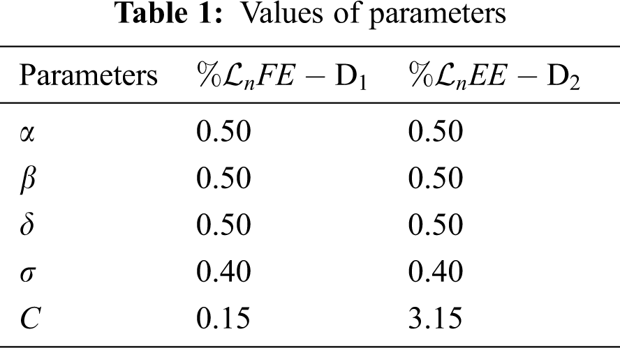
Using the command-built software such as Matlab and simulating the system (1–6) at both equilibria of the model using scientific literature presented in Tab. 1 as follows:

4.1 Euler’s Scheme

The Euler method could be applied to the system (1–5) as follows:

Sn+1=Sn+h(αβ−CInSn−δSn) (11)

Ln+1=Ln+h(CInSn−(σ+δ)Ln) (12)

In+1=In+h(σLn−δIn) (13)

Rn+1=Rn+h((1−α)β−CInRn−δRn) (14)

Qn+1=Qn+h(CInRn−δQn) (15)

where h is any time step size?

4.2 Diagrams

The Euler’s method graphs are plotted for both equilibria of the model as follows:

4.3 Runge-Kutta Scheme

The Runge Kutta method could be applied to the system (1–5) as follows:

Stage I

J1=h(αβ−CInSn−δSn)

K1=h[CInSn−(σ+δ)Ln]

L1=h(σLn−δIn)

M1=h[(1−α)β−CInRn−δRn]

N1=h(CInRn−δQn)

Stage II

J2=h[αβ−C(In+L12)(Sn+J12)−δ(Sn+J12)]

K2=h[C(In+L12)(Sn+J12)−(σ+δ)(Ln+K12)]

L2=h[σ(Ln+K12)−δ(In+L12)]

M2=h[(1−α)β−C(In+L12)(Rn+M12)−δ(Rn+M12)]

N2=h[C(In+L12)(Rn+M12)−δ(Qn+N12)]

Stage III

J3=h[αβ−C(In+L22)(Sn+J22)−δ(Sn+J22)]

K3=h[C(In+L22)(Sn+J22)−(σ+δ)(Ln+K22)]

L3=h[σ(Ln+K22)−δ(In+L22)]

M3=h[(1−α)β−C(In+L22)(Rn+M22)−δ(Rn+M22)]

N3=h[C(In+L22)(Rn+M22)−δ(Qn+N22)]

Stage IV

J2=h[αβ−C(In+L3)(Sn+J3)−δ(Sn+J3)]

K2=h[C(In+L3)(Sn+J3)−(σ+δ)(Ln+K3)]

L2=h[σ(Ln+K3)−δ(In+L3)]

M2=h[(1−α)β−C(In+L3)(Rn+M12)−δ(Rn+M3)]

N2=h[C(In+L3)(Rn+M3)−δ(Qn+N3)]

Final Stage

Sn+1=Sn+16(J1+2J2+2J3+J4) (16)

Ln+1=Ln+16(K1+2K2+2K3+K4) (17)

In+1=In+16(L1+2L2+2L3+L4) (18)

Rn+1=Rn+16(M1+2M2+2M3+M4) (19)

Qn+1=Qn+16(N1+2N2+2N3+N4) (20)

where h is any time step size.

4.4 Diagrams

The Runge Kutta method graphs are plotted for both equilibria of the model as follows:

4.5 NSFD Method

The NSFD method that could be applied to the system (1–5) as follows:

Eq. (1)

Sn+1=Sn+h(αβ−CInSn+1−δSn+1)

Sn+1=Sn+hαβ1+hCIn+hδ (21)

Like, Eq. (21),

Ln+1=Ln+hCInSn1+h(σ+δ) (22)

In+1=In+hσLn1+hδ (23)

Rn+1=Rn+h(1−α)β1+hCIn+hδ (24)

Qn+1=Qn+hCInRn1+hδ (25)

where h is any time step size.

4.6 Stability Results of NSFD Method

Considering the function for the system (3.11–3.15),

M=S+hαβ1+hCI+hδ,P=L+hCIS1+h(σ+δ),U=I+hσL1+hδ,V=R+h(1−α)β1+hCI+hδandW=Q+hCIR1+hδ

The partial derivatives of the Jacobean matrix,

J(S,L,I,R,Q)=[11+hCI+hδ0−hC(S+hαβ)(1+hCI+hδ)200hCI1+h(σ+δ)11+h(σ+δ)hCS1+h(σ+δ)000hσ1+hδ11+hδ0000−hC[R+h(1−α)β](1+hCI+hδ)211+hCI+hδ000hCR1+hδhCI1+hδ11+hδ] (26)

At disease free equilibrium point (S,L,I,R,Q)=(α,0,0,1−α,0) , Eq. (26) becomes

J(α,0,0,1−α,0)=[11+hδ0−hCα(1+hβ)(1+hδ)200011+h(σ+δ)hCα1+h(σ+δ)000hσ1+hδ11+hδ0000−hC(1−α)(1+hβ)(1+hδ)211+hδ000hC(1−α)1+hδ011+hδ]

|J−λI|=0

[11+hδ−λ0−hCα(1+hβ)(1+hδ)200011+h(σ+δ)−λhCα1+h(σ+δ)000hσ1+hδ11+hδ−λ0000−hC(1−α)(1+hβ)(1+hδ)211+hδ−λ000hC(1−α)1+hδ011+hδ−λ]=0

λ1=|11+hδ|<1,λ2=|11+hδ|<1,λ3=|11+hδ|<1

J(α,0,0,1−α,0)=[11+h(σ+δ)hCα1+h(σ+δ)hσ1+hδ11+hδ]

A=TraceofJ,B=DeterminantofJ

A=2+2hδ+hσ(1+hδ)[1+h(σ+δ)],B=1−h2Cασ(1+hδ)[1+h(σ+δ)]

For stability, to prove the following conditions as follows:

     i)   1−A+B>0

    ii)   1+A+B>0

   iii)   B<1

    iv)   1−A+B>0

1−2+2hδ+hσ(1+hδ)[1+h(σ+δ)]+1−h2Cασ(1+hδ)[1+h(σ+δ)]>0

(1+hδ)[1+h(σ+δ)]−2−2hδ−hσ+1−h2Cασ>0

1+hσ+hδ+hδ+h2σδ+h2δ2−2−2hδ−hσ+1−h2Cασ>0

h2(σδ+δ2−Cασ)>0

h2>0.

h>0

Since the step size is never zero, so the condition is satisfied.

(ii) 1+A+B>0

1+2+2hδ+hσ(1+hδ)[1+h(σ+δ)]+1−h2Cασ(1+hδ)[1+h(σ+δ)]>0

(1+hδ)[1+h(σ+δ)]+2+2hδ+hσ+1−h2Cασ>0

1+hσ+hδ+hδ+h2σδ+h2δ2+2+2hδ+hσ+1−h2Cασ>0

h2(σδ+δ2−Cασ)+2h(σ+2δ)+4>0

h2a+2hb+4>0

where a=σδ+δ2−Cασ,b=σ+2δ

h2+2hba+4a>0

h2+2hba+(ba)2+4a>(ba)2

(h+ba)2+4a>(ba)2

Hence, this condition is also satisfied.

(iii)    B<1

1−h2Cασ(1+hδ)[1+h(σ+δ)]<1

1−h2Cασ<(1+hδ)[1+h(σ+δ)]

1−h2Cασ<1+hσ+hδ+hδ+h2σδ+h2δ2

hσ+2hδ++h2σδ+h2δ2+h2Cασ>0

h2(σδ+δ2+Cασ)+h(σ+2δ)>0

h2c+hb>0

where c=σδ+δ2+Cασ

h2+hbc>0

h2+2hb2c+(b2c)2>(b2c)2

(h+b2c)2>(b2c)2

So, condition (iii) is also satisfied, as desired.

4.7 Diagrams

The NSFD method graphs are plotted for both equilibria of the model as follows:

4.8 Comparison Section

5  Results and Concluding Remarks

The simulation of the Euler method is presented in Figs. 1a–1d. Figs. 1b and Fig. 1d show that the system violates the properties of the real-world problem like positivity, boundedness, and dynamical consistency by an increase in the time step size. The Runge Kutta method of order fourth depicts the graphical representation in Figs. 2a–2d, but the technique is time-dependent and converges to the false steady state of the model. The NSFD process depicts the graphical solution of the model in Figs. 3a–3d; the NSFD method converges to proper equilibria of the model at any time step size and fulfils all the model properties. The support comparison of the numerical methods is presented in Figs. 4a–4d. The Euler and RK-4 schemes are dependent on time step size. These numerical schemes are convergent for small step sizes while divergent for large step sizes. But the nonstandard finite difference method used for communication dynamics of leishmaniasis disease is independent of the time step size. It is convergent even for any time step size like hundreds and thousands. NSFD scheme shows positivity, boundedness, and stability and behaves similarly to the behavior of the continuous model. Hence, the NSFD scheme is more efficient, fast convergent, and reliable than the remaining method. In the future, the work will extend to the field as presented in [30–33].

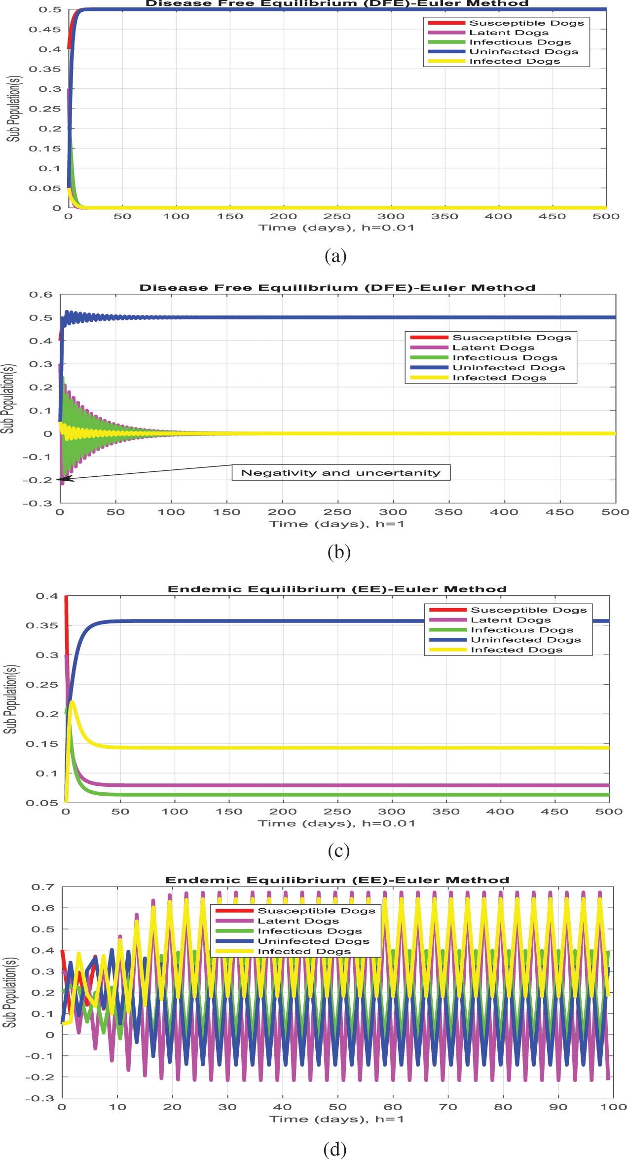
Figure 1: (Euler simulations) subpopulation at LnFE−D1 for h=0.01 (b) subpopulation at LnFE−D1 for h=1 (c) subpopulation at LnEE−D2 for h=0.01 (d) subpopulation at LnEE−D2 for h=1

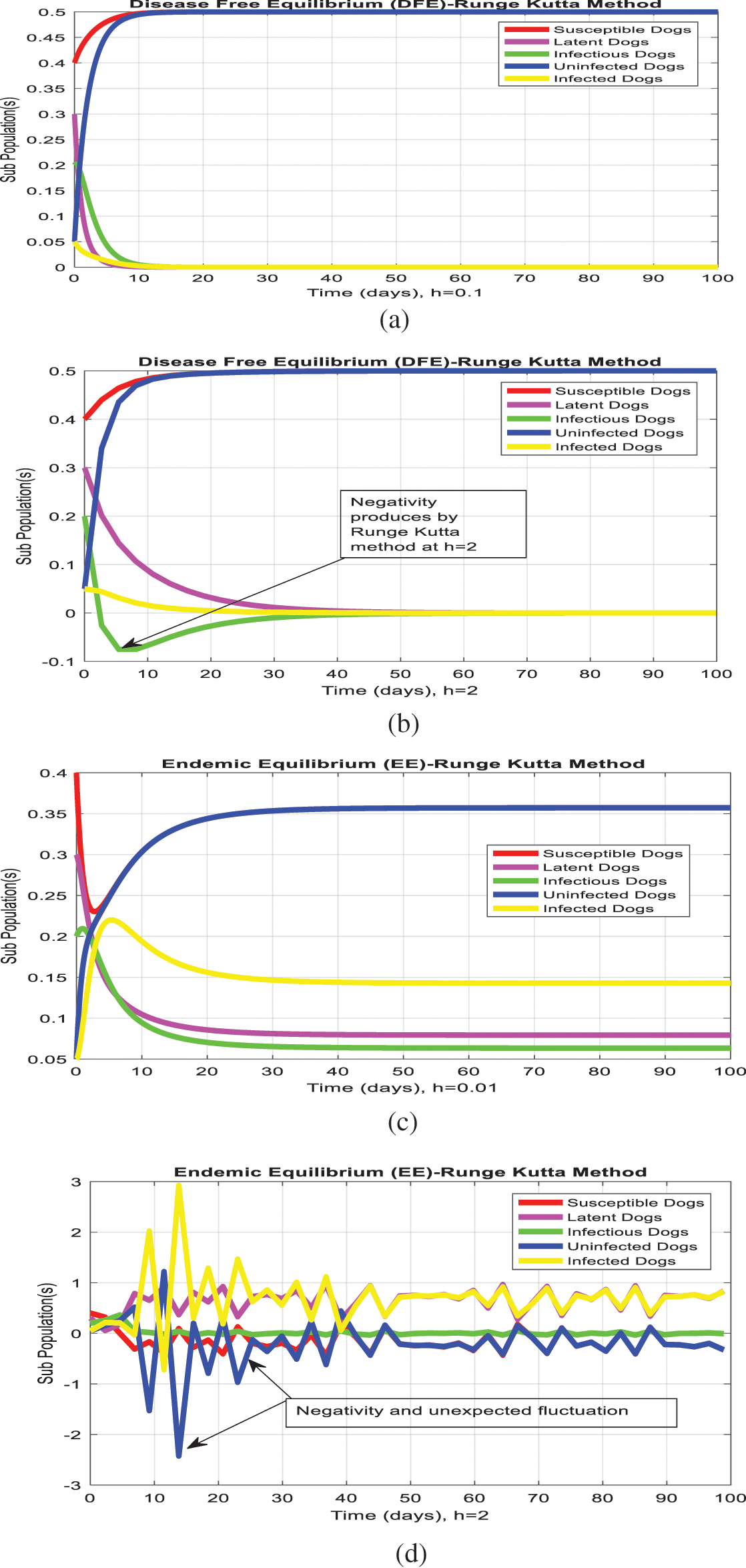
Figure 2: (Runge-Kutta simulations) (a) subpopulation at LnFE−D1 for h=0.1 (b) subpopulation at LnFE−D1 for h=2 (c) subpopulation at LnEE−D2 for h=0.01 (d) subpopulation at LnEE−D2 for h=2

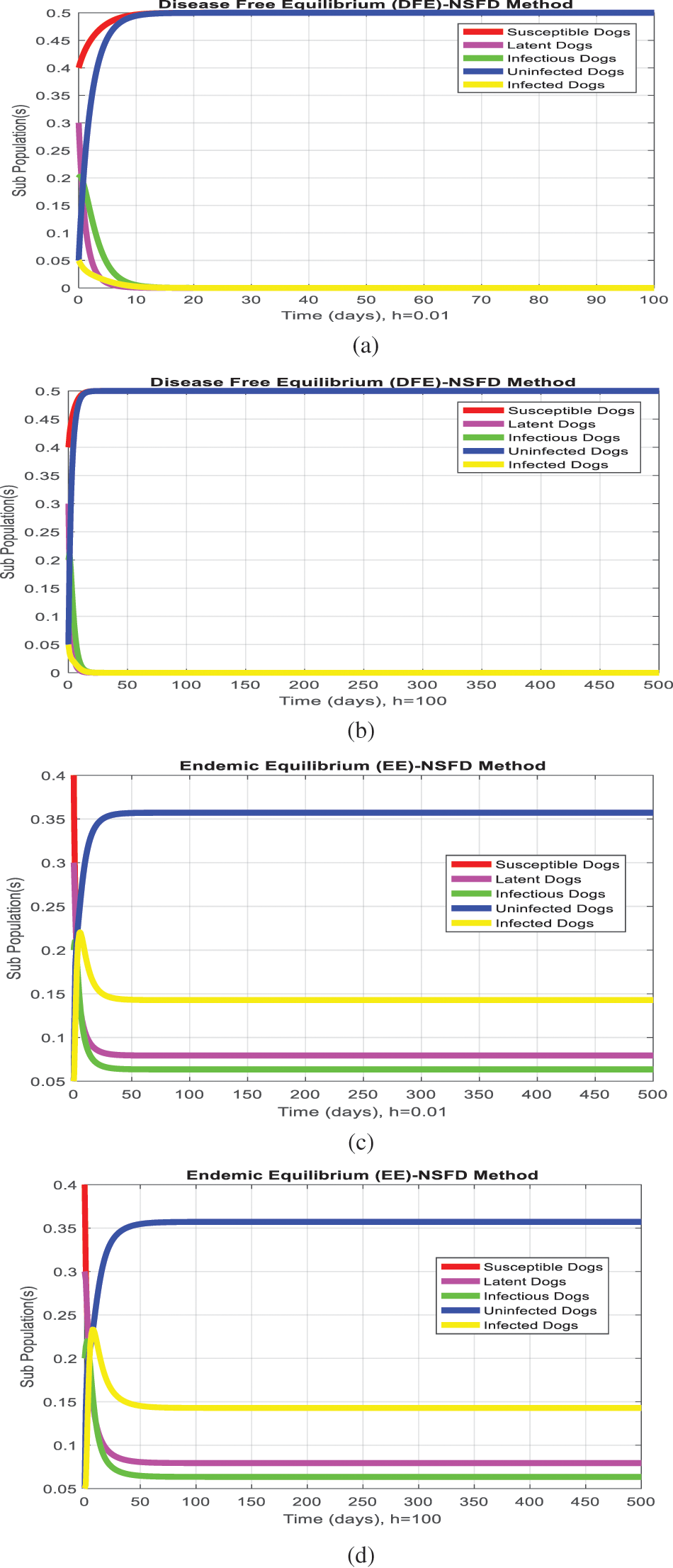
Figure 3: (NSFD simulations) subpopulation at LnFE−D1 for h=0.01 (b) subpopulation at LnFE−D1 for h=100 (c) subpopulation at LnEE−D2 for h=0.01 (d) subpopulation at LnEE−D2 for h=100

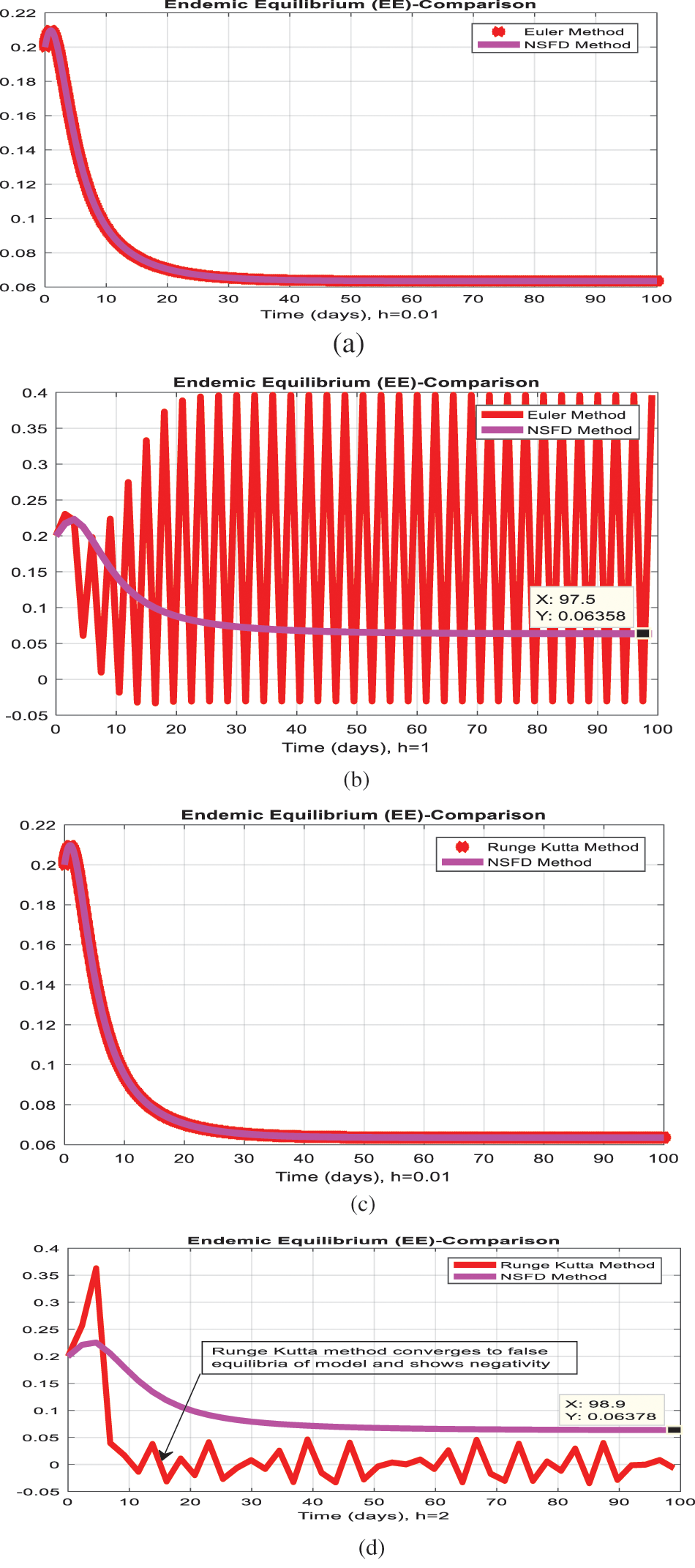
Figure 4: Comparison of methods (a) infected humans at LnEE−D2 for h=0.01 (b) infected humans at LnEE−D2 for h=1 (c) infected humans at LnEE−D2 for h=0.01 (d) infected humans at LnEE−D2 for h=2

Acknowledgement: The authors are thankful to the Govt. of Pakistan for providing the facility to conduct the research. All Authors are grateful for the suggestions of anonymous referees to improve the quality of the manuscript.

Funding Statement: The authors received no specific funding for this study.

Conflicts of Interest: The authors declare that they have no conflicts of interest to report regarding the present study.

References

 1.  F. Boukhalfa, M. Helal and A. Lakmeche, “Mathematical analysis of visceral leishmaniasis model,” Research in Applied Mathematics, vol. 1, no. 1, pp. 01–06, 2017. [Google Scholar]

 2.  L. E. Coffeng, E. A. L. Rutte, J. Muñoz, E. R. Adams, J. M. Prada et al., “Impact of changes in detection effort on control of visceral leishmaniasis in the Indian subcontinent,” The Journal of Infectious Diseases, vol. 221, no. 5, pp. 546–553, 2019. [Google Scholar]

 3.  V. Gandhi, N. S. A. Salti and I. M. Elmojtaba, “Mathematical analysis of a time delay visceral leishmaniasis model,” Journal of Applied Mathematics and Computing, vol. 63, no. 1, pp. 217–237, 2020. [Google Scholar]

 4.  M. Zamir, F. Nadeem and G. Zaman, “Optimal control of visceral, cutaneous and post kala-azar leishmaniasis,” Advances in Difference Equations, vol. 20, no. 1, pp. 01–23, 2020. [Google Scholar]

 5.  F. Nadeem, M. Zamir and A. Tridane, “Modeling and control of zoonotic cutaneous leishmaniasis,” Punjab University Journal of Mathematics, vol. 51, no. 2, pp. 01–12, 2019. [Google Scholar]

 6.  E. A. L. Rutte, E. E. Zijlstra and S. J. D. Vlas, “Post-kala-azarkala-azar dermal leishmaniasis as a reservoir for visceral leishmaniasis transmission,” Trends in Parasitology, vol. 35, no. 8, pp. 590–602, 2019. [Google Scholar]

 7.  L. Adamu and N. Hussaini, “An epidemic model of zoonotic visceral leishmaniasis with time delay,” Journal of the Nigerian Society of Physical Sciences, vol. 19, no. 1, pp. 20–29, 2019. [Google Scholar]

 8.  M. Zamir, G. Zaman and A. S. Alshomrani, “Control strategies and sensitivity analysis of anthroponotic visceral leishmaniasis model,” Journal of Biological Dynamics, vol. 11, no. 1, pp. 323–338, 2017. [Google Scholar]

 9.  H. J. Shimozako, J. Wu and E. Massad, “Mathematical modelling for zoonotic visceral leishmaniasis dynamics: A new analysis considering updated parameters and notified human Brazilian data,” Infectious Disease Modelling, vol. 2, no. 2, pp. 143–160, 2017. [Google Scholar]

10. I. Ghosh, T. Sardarand and J. A. Chattopadhyay, “Mathematical study to control visceral leishmaniasis: An application to South Sudan,” Bulletin of Mathematical Biology, vol. 79, no. 5, pp. 1100–1134, 2017. [Google Scholar]

11. M. E. Lmojtaba, S. Biswas and J. Chattopadhyay, “Global analysis and optimal control of a periodic visceral leishmaniasis model,” Mathematics, vol. 5, no. 4, pp. 01–80, 2017. [Google Scholar]

12. S. Biswas, “Mathematical modeling of visceral leishmaniasis and control strategies,” Chaos, Solitons & Fractals, vol. 17, no. 104, pp. 546–556, 2017. [Google Scholar]

13. S. Debroy, O. Prosper, A. Mishoe and A. Mubayi, “Challenges in modeling complexity of neglected tropical diseases: A review of dynamics of visceral leishmaniasis in resource-limited settings,” Emerging Themes in Epidemiology, vol. 14, no. 1, pp. 01–04, 2017. [Google Scholar]

14. E. A. L. Rutte, L. A. Chapman, L. E. Coffeng, S. Jervis, E. C. Hasker et al., “Elimination of visceral leishmaniasis in the Indian subcontinent: A comparison of predictions from three transmission models,” Epidemics, vol. 17, no. 18, pp. 67–80, 2017. [Google Scholar]

15. L. Zou, J. Chen and S. Ruan, “Modeling and analyzing the transmission dynamics of visceral leishmaniasis,” Mathematical Biosciences and Engineering, vol. 14, no. 5, pp. 1500–1585, 2017. [Google Scholar]

16. N. Siewe, A. A. Yakubu, A. R. Satoska and A. Friedman, “Immune response to infection by leishmania: A mathematical model,” Mathematical Biosciences, vol. 16, no. 276, pp. 28–43, 2016. [Google Scholar]

17. K. S. Rock, R. J. Quinnell, G. F. Medley and O. Courtenay, “Progress in the mathematical modelling of visceral leishmaniasis,” Advances in Parasitology, vol. 16, no. 94, pp. 49–131, 2016. [Google Scholar]

18. P. K. Roy, D. Biswas and F. A. Basir, “Transmission dynamics of cutaneous leishmaniasis: A delay-induced mathematical study,” Journal of Medical Research and Development, vol. 4, no. 2, pp. 11–23, 2015. [Google Scholar]

19. A. Subramanian, V. Singh and R. R. Sarkar, “Understanding visceral leishmaniasis disease transmission and its control: A study based on mathematical modelling,” Mathematics, vol. 3, no. 3, pp. 913–944, 2015. [Google Scholar]

20. G. F. Medley, T. D. Hollingsworth, P. L. Olliaro and E. R. Adams, “Health-seeking behaviour, diagnostics and transmission dynamics in the control of visceral leishmaniasis in the Indian subcontinent,” Nature, vol. 528, no. 7580, pp. 102–108, 2015. [Google Scholar]

21. F. M. Allehiany, F. Dayan, F. F. Al-Harbi, N. Althobaiti, N. Ahmed et al., “Bio-inspired numerical analysis of COVID-19 with fuzzy parameters,” Computers, Materials & Continua, vol. 72, no. 2, pp. 3213–3229, 2022. [Google Scholar]

22. Z. Iqbal, N. Ahmed, D. Baleanu, W. Adel, M. Rafiq et al., “Positivity and boundedness preserving numerical algorithm for the solution of fractional nonlinear epidemic model of HIV/AIDS transmission,” Chaos, Solitons & Fractals, vol. 134, no. 1, pp. 01–19, 2020. [Google Scholar]

23. Y. T. Mangongo, J. D. K. Bukweli and J. D. B. Kampempe, “Fuzzy global stability analysis of the dynamics of malaria with fuzzy transmission and recovery rates,” American Journal of Operations Research, vol. 11, no. 6, pp. 257–282, 2021. [Google Scholar]

24. M. Jawaz, N. Ahmed, D. Baleanu, M. Rafiq and M. A. Rehman, “Positivity preserving technique for the solution of HIV/AIDS reaction-diffusion model with time delay,” Frontiers in Physics, vol. 7, no. 1, pp. 01–10, 2020. [Google Scholar]

25. N. Ahmed, M. Rafiq, W. Adel, H. Rezazadeh, I. Khan et al., “Structure preserving numerical analysis of HIV and CD4+ T-cells reaction-diffusion model in two space dimensions,” Chaos, Solitons & Fractals, vol. 139, no. 1, pp. 01–18, 2020. [Google Scholar]

26. A. Raza, J. Awrejcewicz, M. Rafiq, N. Ahmed, M. S. Ahsan et al., “Dynamical analysis and design of computational methods for nonlinear stochastic leprosy epidemic model,” Alexandria Engineering Journal, vol. 61, no. 10, pp. 8097–8111, 2022. [Google Scholar]

27. A. Raza, M. Rafiq, J. Awrejcewicz, N. Ahmed and M. Mohsin, “Stochastic analysis of nonlinear cancer disease model through virotherapy and computational methods,” Mathematics, vol. 10, no. 3, pp. 01–18, 2022. [Google Scholar]

28. A. Raza, M. Rafiq, J. Awrejcewicz, N. Ahmed and M. Mohsin, “Dynamical analysis of coronavirus disease with crowding effect, and vaccination: A study of third strain,” Nonlinear Dynamics, vol. 107, no. 4, pp. 3963–3982, 2022. [Google Scholar]

29. A. Raza, J. Awrejcewicz, M. Rafiq and M. Mohsin, “Breakdown of a nonlinear stochastic Nipah virus epidemic model through efficient numerical methods,” Entropy, vol. 23, no. 12, pp. 01–20, 2021. [Google Scholar]

30. M. A. Akbar, L. Akinyemi, S. W. Yao, A. Jhangeer, H. Rezazadeh et al., “Soliton solutions to the boussinesq equation through Sine-Gordon method and Kudryashov method,” Results in Physics, vol. 25, no. 1, pp. 01–19, 2021. [Google Scholar]

31. I. Ahmad, M. N. Khan, M. Inc, H. Ahmad and K. S. Nisar, “Numerical simulation of simulate an anomalous solute transport model via local meshless method,” Alexandria Engineering Journal, vol. 59, no. 4, pp. 2827–2838, 2020. [Google Scholar]

32. H. Ahmad and T. A. Khan, “Variational iteration algorithm-I with an auxiliary parameter for wave-like vibration equations,” Journal of Low Frequency Noise, Vibration and Active Control, vol. 38, no. 3, pp. 1113–1124, 2019. [Google Scholar]

33. H. Ahmad, T. A. Khan, P. S. Stanimirovic and I. Ahmad, “Modified variational iteration technique for the numerical‎ solution of fifth-order KdV-type equations,” Journal of Applied and Computational Mechanics, vol. 6, no. 20, pp. 1220–1227, 2020. [Google Scholar]