Nonlinear Dynamic System Identification of ARX Model for Speech Signal Identification

1  Introduction

System identification problem has been approached for the last two to three decades by many researchers using Artificial Neural Networks (ANN) as these networks can be designed to be used as stable universal approximators [1]. Some of the earliest works in system identification were attempted with the adaptive algorithms measuring Least Mean Squares (LMS) and its variants [2–4]. Further neural networks in terms of Functional Link Artificial Neural Networks (FLANN) have been used by many researchers [5–8]. Blackbox modeling is the process of the unknown behavior of a system’s modeling. Currently many researchers have been inclined to solve nonlinear dynamic system identification problems since they represent some of the most important applications in the field of engineering. Many authors have applied Multilayer Perception (MLP) in the solution of nonlinear system identification problems using dynamic gradient descent algorithm [9–11]. It has been found that, a complex nonlinear system identification problem computation is a challenging and time-consuming procedure using the MLP and the training in such cases becomes very slow. The Radial Basis Functions Neural Network (RBFNN) became popular as it offers fast online learning with good generalization, and input noise tolerance capacity, [12–16]. A nonlinear dynamic system identification using Fusion kernel-based RBFN is proposed in [17]. Autoregressive (AR) along with the RBFNN model has been used to estimate the parameters of linear and nonlinear systems [18]. Authors have proposed parameter estimation of Autoregressive with Exogenous terms (ARX) model using Recurrent Neural Network (RNN), which shows the performance is better than the existing Neural Network models [19,20]. In addition, for nonlinear dynamic system identification challenges, a Deep Convolutional Neural Network (DCNN) model is proposed in [21] where the results indicate the models perform better than MLP and basic FLANN. One of the major drawbacks of the RNN model during training is the vanishing gradient problem which occurs because RNN needs the backpropagation to update the weights every iteration. Recently Long-Short Term Memory (LSTM), an improved version of RNN, become popular since it overcomes the vanishing gradient problem and hence many authors have used it in different applications such as time series modelling, speech recognition, natural language processing, and sequence prediction [22,23]. Further, the concept of bi-directional and uni-directional LSTM is presented in [24], where it has been illustrated that the uni-directional LSTM can recognize longer sequences as time series problems. The Bidirectional LSTM (Bi-LSTM) networks have the ability to train the input data in the forward and backward directions. which prove to be advantageous in applications like speech recognition, because it can train the model twice, in the forward and backward directions, as presented in [25]. A Deep Speech network architecture with pseudo-LSTM operation is presented in [26]. Furthermore, investigations have been carried out on LSTM, Bi-LSTM, and the works are presented in [27–31].

Some of the recent challenging applications of system identification are found in the area of industrial biomedical and speech modelling. The natural speech signal may be either non-linear or non-stationary or both. Although certain models have been designed for biomedical signals and speech signals, the current research lacks the estimation of different parameters.

In this paper, we have considered the parameter estimation of the speech signals using various deep neural network models. A speech signal is recorded using Audacity Software and used as a nonlinear ARX model for the nonlinear dynamic system identification problem. Initially, the speech signal is passed through RNN and LSTM networks. To make it more accurate the model Bi-directional LSTM model is considered since it can train the model twice. After achieving good performance finally, a Deep stack Bi-LSTM architecture is proposed. The architecture consists of 5 layers including 3 Bi-LSTM layers. To determine the superiority of the proposed model, a comparison is made between RNN and Bi-LSTM. Though many problems have been solved in system identification and its variants, all the applications are mostly industry-based. However, in this work, the model has been developed by considering the recorded speech signal, which is the new incite of this work. Another novelty of the model is that it is developed with a Bi-LSTM deep learning model which is rare for the field of parameter estimation of the speech signals both voiced and unvoiced speech signals can also be modelled in this proposed system.

The rest of the paper is arranged as follows. In Part 2 the ARX Speech Modelling is formulated. In Part 3, the background of the proposed model is briefly presented. In Part 4, the proposed model and its architecture are presented. In Part 5, the results and analysis are provided. Finally, the conclusion and the scope of future research are presented in Part 6.

2  Theoretical Background

ARX Speech Modelling

The behaviour of the speech can be modelled using an all-pole filter. A pole-zero filter is a better approximation for nasals or nasalized vowels in the open phase model, an unknown source is used to excite a time-varying pole-zero filter. The speech signal can be modelled as a time-variant pole-zero system with an equation error or Auto-Regressive Exogenous (ARX) model, it is formulated as:

Y(n)+∑i=1P⁡wi(n)s(n−i)=∑j=1q⁡wj(n)X(n−j)+X(n)+e(n) (1)

where Y(n) , X(n) are observed speech output and input form, wi(n) and wi(n) are the time-varying coefficient. The model order is denoted as p,q, and e(n) , denoted as the error of the model. Further X(n) can be defined as:

X(n)=XY(n)+Xn(n) (2)

where XY(n) is defined as the voice source signal with radiation characteristics of the lips are included and Xn(n) is denoted as additive independent white noise. So, Eq. (1) is further defined as:

Y(n)+∑i=1P⁡wi(n)s(n−i)=∑j=1q⁡wj(n)XY(n−j)+∑j=1q⁡wj(n)Xn(n−j)+XY(n)+Xn(n)+e(n) (3)

Now let

ε(n)=∑j=1q⁡wj(n)Xn(n−j)+Xn(n)+e(n) (4)

Then,

Y(n)+∑i=1P⁡wi(n)Y(n−j)=∑j=1q⁡wj(n)XY(n−j)+ε(n) (5)

3  Proposed Methodology

3.1 Long-Short Term Memory (LSTM)

LSTM is an extended version of RNN which was to addresses the shortcomings of RNNs, like vanishing gradients. In many scenarios, RNN is unable to accurately capture non-stationary relationships that occur over time. A method to solve the above problem by adding a memory along with general RNNs has been presented in [25]. This network employs continuous jump connections for capturing complex dependencies and provides a memory capacity that allows the data from previous time steps to be analyzed without traversing the whole network. The main difficulty with skip connections is whether they are primarily introduced for short-term or long-term dependency. Authors in the survey have been studied the superiority of RNN in the applications of predicting dynamic systems, where time-variant models are exposed to stationary or non-stationary short-term dependencies [32]. From Fig. 1 it can be seen that LSTM contains three gates, where the first is the input gate, the second, is a forget gate and the third is an output gate. The changes on the cell state vector are possible due to the presence of these gates, which are used to capture long-term dependencies. The cell allows the network to remember some time depending on different properties, allowing the information flow to be controlled. The main objective of LSTM includes modelling of long-term dependencies, which has been introduced in [30].

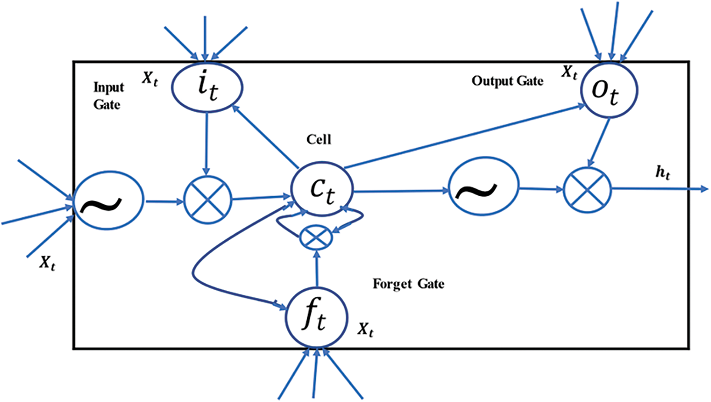
Figure 1: LSTM cell

The gates work by adding or removing information by controlling the flow of data into and out of the cell, allowing the cell to remember values across arbitrary time intervals. The working of gates can be formulae as, at the time(t), the unit components of the LSTM structure are updated as:

it=σ(wxixt+whiht−1+wcict−1+bi) (6)

ft=σ(wxfxt+whfht−1+wcfct−1+bf) (7)

ot=σ(wxoxt+whoht−1+wcoct−1+bo) (8)

Ct=ftct−1+ittanh(wxcxt+whcht−1+bc) (9)

ht=ottanh⁡(ct) (10)

where σ(∙) is denoted as sigmoid activated function and i,f,o,x, and c, are denoted as input, forget, output, cell input activation, and cell state vector, gates respectively all of them are having the same size as hidden vector h. The matrix weight is defined as Wci,Wcf,Wci.

3.2 Bi-Directional Long-Short Term Memory (BI-LSTM)

The principle of Bidirectional LSTM is to train the neural network by reading the training input in two directions [27]. Two-way LSTM reads training data in the direction of two-time, then trains the data. By connecting the left and right summary vectors, the two-dimensional LSTM prediction process is completed. In comparison to other unidirectional deep neural architectures, Bi-directional LSTM archives perform exceptionally well since it incorporates both left and right context information, as presented in [25] Bidirectional LSTM networks are distinguished by the fact that they propagate the state vector not only forward but also backward. As a result of the reverse state propagation, both directions of time are taken into account, and current outputs can be included in projected future correlations. As a result, compared to unidirectional LSTM networks, Bidirectional LSTM networks can detect and extract more time dependencies and resolve them more precisely [28]. Bidirectional LSTM networks, according to the authors, encapsulate geographically and temporally scattered information by adopting a flexible cell state vector propagation strategy to handle partial input [29].

4  Proposed Deep Stacked Bi-LSTM Architecture

4.1 Input Layer

The model’s input is the original speech signal recorded in matrix laboratory (MATLAB) 2021a software. The total no of data set is 263280. The data is divided 70:30 ratio for the training and testing process. The training sample is 184297. So total X = ( X1,X2…,Xt,Xt+1,…X263280 ). The architectural details of the proposed model are presented in Table 1

4.2 Bi-LSTM Network Layers

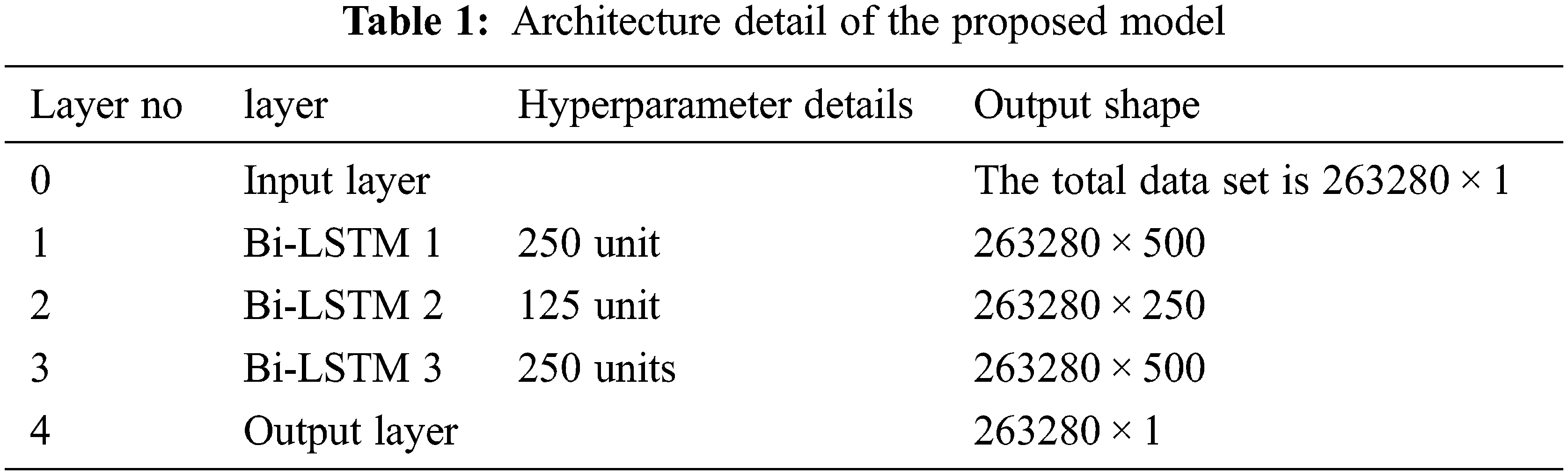
In this work, three layers of Bi-LSTM are designed. In the first Bi-layer 250 cells of LSTM on each hidden layer of LSTM, such as 500 hidden cells of LSTM is considered. Similarly, for the second Bi-layer 125 LSTM cells, and the third Bi-LSTM layer 250 LSTM cells are designed. After trial-and-error attempts, these cells were fixed as they provided better results and make the training process error-free with less time. These samples were passed through a fully connected layer followed by an output layer. This method is the extended version of the traditional RNN. The proposed architecture is designed with triple Bi-layer stacked with each other. The Bi-LSTM is based on the idea of a bidirectional RNN that can run LSTM cells both forward and backward. Additionally, it divides the overall data into two hidden layers at each time step. The major advantage of the proposed method is, that by using prior and future data information forward and backward hidden sequences of data can be computed. The element-wise sum approach is used to integrate these hidden properties.

4.3 Fully Connected Layer with the Output Layer

It is the last layer, which is a fully connected layer. After the third Bi-LSTM, the outcomes are recorded in this layer. To avoid overfitting problems a dropout method is applied. As the total input size of the speech signal is 263280 × 1 then the expected outcome should also 263280 × 1. Then the error is calculated by the difference between actual and predicted output. The basic architecture of the proposed Deep stacked Bi-LSTM is shown in Fig. 1. Where the input layer is denoted as X=(X0…Xt…Xt+1…X263280) followed by 1st Bi-layer, 2nd Bi-layer, and 3rd Bi-layer. The final layer is the output layer. The proposed Stacked Bi-LSTM is depicted in Fig. 2.

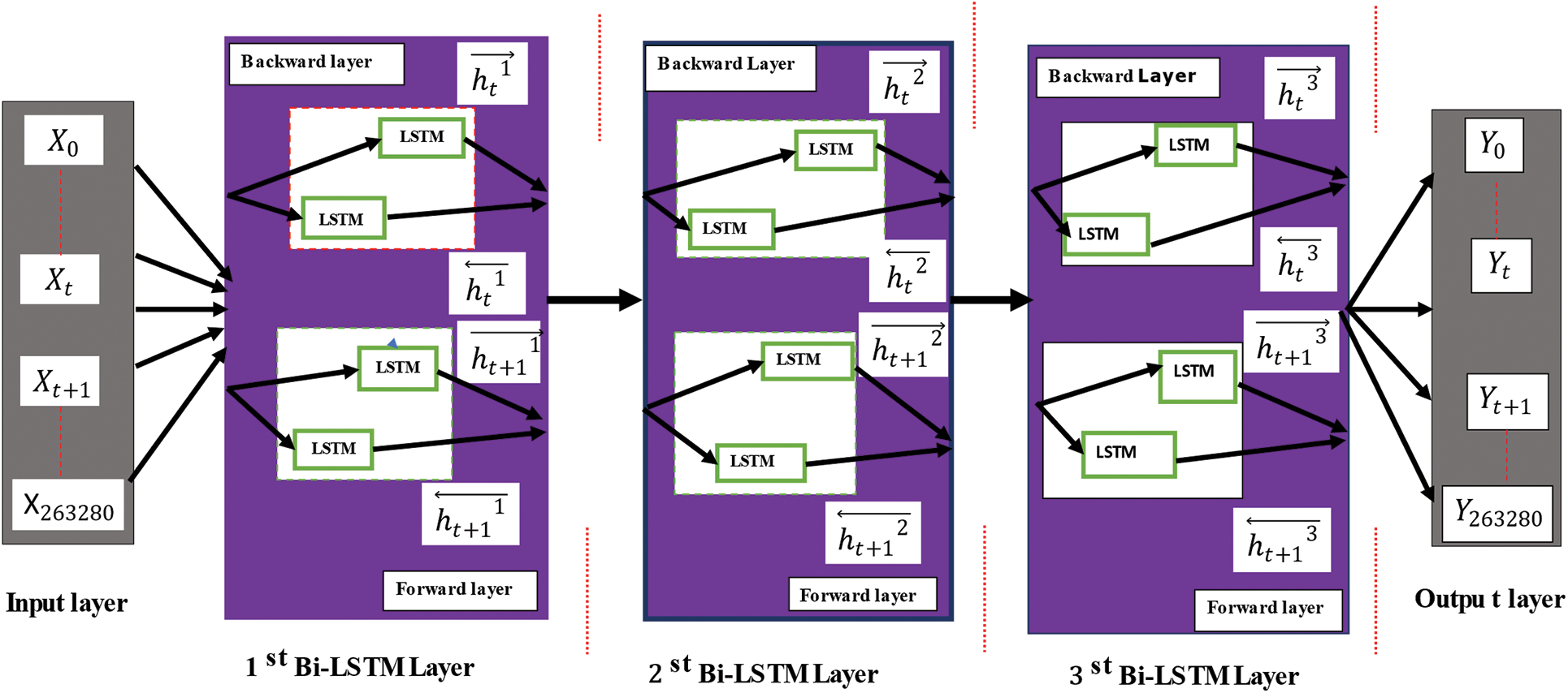
Figure 2: Basic architecture of deep stacked Bi-LSTM

The working of gates forward and backward process is depicted in Fig. 3. To obtain previous stage information, the input data is been passed through hidden layers in the forward direction. Similarly, the input sequence is processed through the hidden layers in the reverse direction to gain information for the next stage. To get contextual information, the lower hierarchies of the model output are taken by the hidden layers in the higher hierarchies of the model.

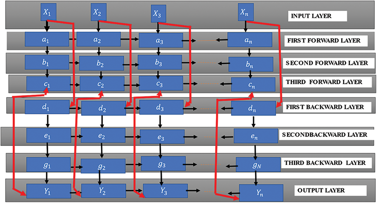
Figure 3: The three-layer stacked bidirectional LSTM’s general structure

The following formula is used to find the concealed state information at for the first forward layer:

it(a)=σ(wi(a)at−1+hi(a)Xt+bi(a)) (11)

ft(a)=σ(wf(a)at−1+hf(a)Xt+bf(a)) (12)

ot(a)=σ(wo(a)at−1+ho(a)Xt+bo(a)) (13)

ut(a)=tan⁡h(wu(a)at−1+hu(a)Xt+bu(a)) (14)

Ct(a)=it(a)out(a)+ft(a)oCt−1(a) (15)

at=ot(a)otan⁡h(Ct(a)) (16)

The following formula is used to find the concealed state information bt for the second forward layer:

it(b)=σ(wi(b)bt−1+hi(b)at+bi(b)) (17)

ft(b)=σ(wf(b)bt−1+hf(b)at+bf(b)) (18)

ot(b)=σ(wo(b)bt−1+ho(b)at+bo(b)) (19)

ut(b)=tan⁡h(wu(b)bt−1+hu(b)at+bu(b)) (20)

Ct(b)=it(b)out(b)+ft(b)oCt−1(b) (21)

bt=ot(b)otan⁡h(Ct(b)) (22)

The following formula is used to find the concealed state information ct for the third forward layer:

it(C)=σ(wi(C)Ct−1+hi(b)bt+bi(b)) (23)

ft(C)=σ(wf(C)Ct−1+hf(C)bt+bf(C)) (24)

ot(C)=σ(wo(C)Ct−1+ho(C)bt+bo(C)) (25)

ut(C)=tan⁡h(wu(C)ct−1+hu(C)bt+bu(C)) (26)

Ct(C)=it(C)out(C)+ft(C)oCt−1(C) (27)

Ct=ot(C)otan⁡h(Ct(C)) (28)

Identification of the hidden state information dt for first backward layer is formulated as:

it(d)=σ(wi(d)dt+1+hi(d)Xt+bi(d)) (29)

ft(d)=σ(wf(d)dt+1+hf(d)Xt+bf(d)) (30)

ot(d)=σ(wo(d)dt+1+ho(d)Xt+bo(d)) (31)

ut(d)=tan⁡h(wu(d)dt+1+hu(d)Xt+bu(d)) (32)

Ct(d)=it(d)out(d)+ft(d)oCt−1(d) (33)

dt=ot(d)otan⁡h(Ct(d)) (34)

Identification of the hidden state information et for the second backward layer is formulated as:

it(e)=σ(wi(e)et+1+hi(e)dt+bi(e)) (35)

ft(e)=σ(wf(e)et+1+hf(e)dt+bf(e)) (36)

ot(e)=σ(wo(e)et+1+ho(e)dt+bo(e)) (37)

ut(e)=tan⁡h(wu(e)et+1+hu(e)dt+bu(e)) (38)

Ct(e)=it(e)out(e)+ft(e)oCt−1(e) (39)

et=ot(e)otan⁡h(Ct(e)) (40)

Identification of the hidden state information gt for the second backward layer is formulated as:

it(g)=σ(wi(g)gt+1+hi(g)et+bi(g)) (41)

ft(g)=σ(wf(g)gt+1+hf(g)et+bf(g)) (42)

ot(g)=σ(wo(g)et+1+ho(g)et+bo(g)) (43)

ut(g)=tan⁡h(wu(g)gt+1+hu(g)et+bu(g)) (44)

Ct(g)=it(g)out(g)+ft(g)oCt−1(g) (45)

gt=ot(g)otan⁡h(Ct(g)) (46)

For every time step ( t ), the further step or output is obtained by concatenating hidden state information ( ct ). The next forward layer or in this case third forward layer and the hidden state information ( gt ) for the third backward layer. The final step is formulated as:

Yt=h(Y)Ct+w(Y)Ct+b(Y) (47)

In this work, the advantages of Bi-LSTM over unidirectional LSTM are considered. In bidirectional, there are two directions to preserve the future and the past information for input, which is a unique advantage over a unidirectional LSTM [23]. In unidirectional LSTM the input flows in one direction eighter backward or forward. In Bi-LSTM one more LSTM layer is added to reverse the direction of information flow. That means the input flows backward in the additional LSTM layer [26]. Finally, the combination of output from both LSTM layers in several ways like average, sum, multiplication, or concatenation. After the application of LSTM twice in the algorithm, learning long-term dependencies and thus consequently will improve the accuracy of the model. Further, the layer of additional LSTM is increased to achieve better results. In this work, a Deep Bi-LSTM is proposed with 3 Bi-LSTM layers were considered. First Bi-LSTM model feeds data to an LSTM model (feedback layer) and then repeats the training via another LSTM model on the reverse of the sequence of input data. From the observation, it is analysed that BI-LSTM can capture underlying context better by traversing inputs data twice (from left to right and then from right to left). From the comparison table, the behavioural analysis comparing both the unidirectional LSTM and Bi-LSTM is presented.

5  Results and Discussion

In this section, a nonlinear system example is taken for identification and their performance is compared with the proposed model and basic RNN, LSTM models. For analysis, a speech signal as a nonlinear signal is considered. The comparison between different models is done based on a differential matrix of MSE and RMSE, which is formulated as:

MSE=1N∑i=1N⁡(Ti−pi)2 (48)

RMSE=∑i=1N⁡(Ti−pi)2  (49)

Data set: Speech Signal

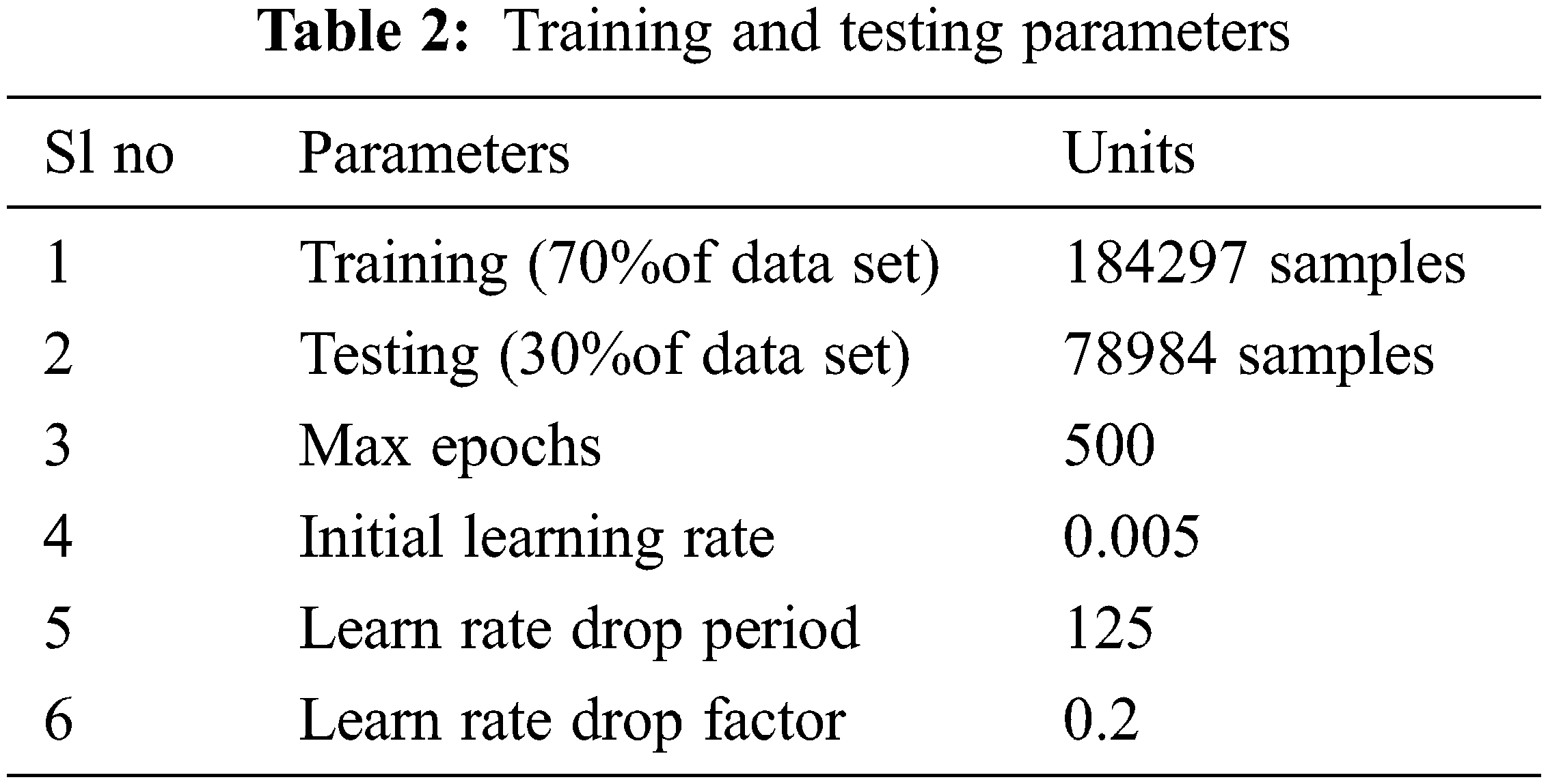
Natural speech signals are nonlinear and dynamic. These signals are a non-stationary and one-dimensional function of time. The data set is prepared with 200 speech signals collected from different persons of Siksha “O” Anusandhan University, Bhubaneswar. A sample from the data set is shown in Fig. 4. To instigate the superiority of the proposed model, a speech signal is recorded by using Audacity software. The recorded signal is “HELLO HELLO GOOD MORNING TO ALL OF YOU WELCOME TO SIKSHA ‘O’ ANUSANDHAN UNIVERSITY”. The length of the recorded speech is 263280 samples, among them for training 70% of the total data, that is 184292 samples, and for testing 78979 samples are taken. The results are generated with the MATLAB 2021a platform. From Table 2 the parameters of the proposed architecture for training are presented. Where the initial learning rate is 0.005, Learn Rate Drop Period is 125. The maximum epoch taken is 500. The Recorded speech “HELLO HELLO GOOD MORNING TO ALL OF YOU WELCOME TO SIKSHA ‘O’ ANUSANDHAN UNIVERSITY” is depicted in Fig. 4.

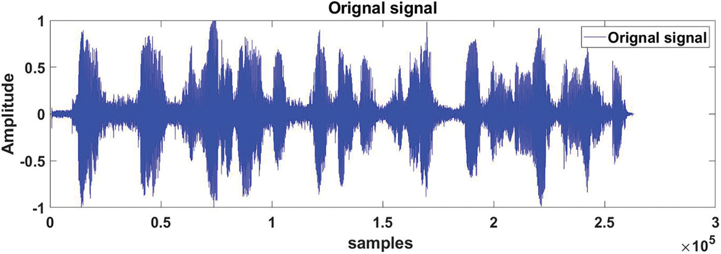
Figure 4: Recorded speech “HELLO HELLO GOOD MORNING TO ALL OF YOU WELCOME TO SIKSHA ‘O’ ANUSANDHAN UNIVERSITY”

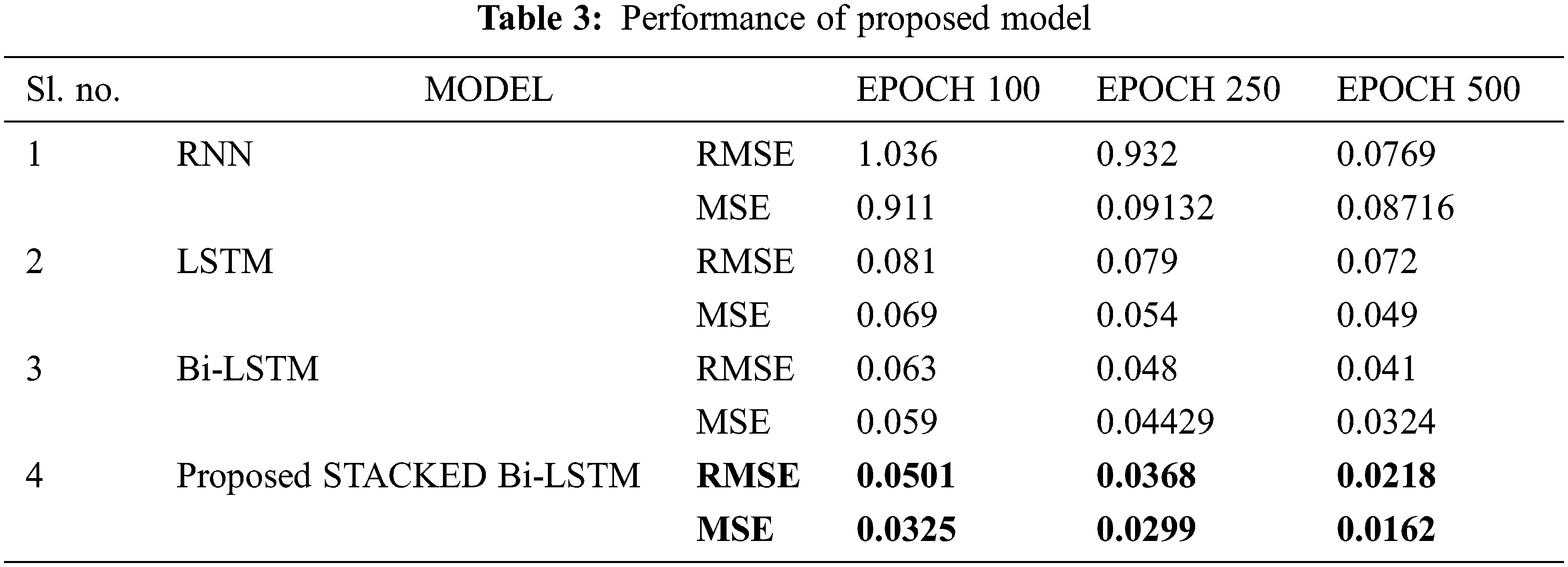
From Table 3, it is observed that the RNN model is providing more RMSE in comparison to other models considered. In this work, the speech signals are considered with a length of 263280. RNN models have a vanishing gradient problem due to the large size of the data. The LSTM is providing a better result than that of simple RNN as it is not affected by the vanishing gradient problem. In Bi-LSTM, there are two directions to preserve the future and the past information for input, which is a unique advantage over the LSTM model. The lower RMSE values are obtained from the proposed stacked Bi-LSTM as the number of features increases while increasing the number of layers which is making the training more robust than other models. The performance of the proposed model can be seen in Fig. 9. From Table 2 the parameters used for training the model are presented.

Figs. 5 and 6 present the actual vs. predicted output of Bi-LSTM model training and testing results.

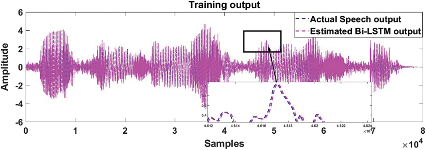
Figure 5: The actual vs. predicted training output between actual speech and Bi-LSTM model output is presented

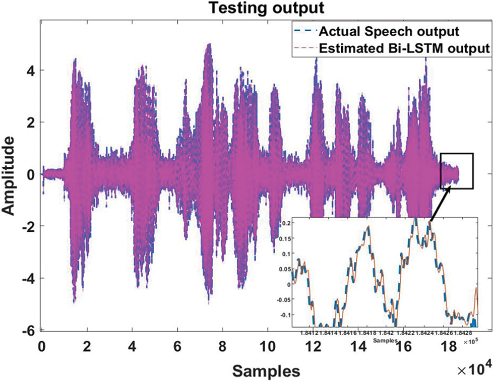
Figure 6: The actual vs. predicted training output between actual speech and Bi-LSTM model output is presented

Figs. 7 and 8 present the actual vs. predicted output of proposed Stacked Bi-LSTM model training and testing results.

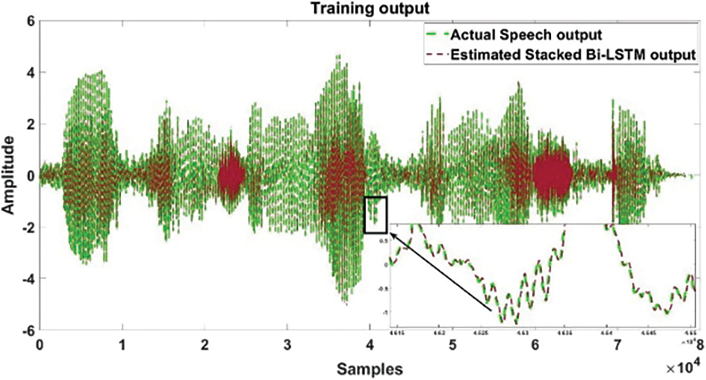
Figure 7: The actual vs. predicted training output between actual speech and proposed Stacked Bi-LSTM model output is presented

Figure 8: The actual vs. predicted testing output between actual speech and proposed Stacked Bi-LSTM model output is presented

The cast function of the prosed model is depicted in Fig. 9. The curve of RMSE shows better training performance of the proposed model as the no of epochs increases.

Figure 9: The cost function showing RMSE error performance curve

From Table 3, the proposed model’s performance is examined. A comparison of models is taken between the Basic RNN, Unidirectional LSTM, Bi-LSTM, and proposed Stacked Bi-LSTM Model. For the initial case 100 epochs are taken for training the model where RNN archive1.036 RMSE and 0.911 MSE, LSTM archive 0.081 RMSE and 0.069 MSE, BI-LSTM is archive 0.063 RMSE and 0.059 MSE. Similarly, the epochs were increased periodically from 250 to 500.The result obtained after 250 epoch, RNN 0.932 RMSE and 0.09132 MSE, LSTM 0.079 RMSE and 0.054 MSE, BI-LSTM 0.048 RMSE and 0.04429 MSE. Finally, the maximum no of epochs increased to 500 and the obtained results are RNN 0.0769 RMSE and 0.08716 MSE, LSTM 0.72 RMSE, and 0.049 MSE, BI-LSTM 0.041 RMSE, and 0.0324 MSE. The outcome of the performance analysis is, that by improving the RNN architecture the Bi-LSTM provides better results than the basic RNN. By increasing the no of the epoch, the performance of the Bi-LSTM is increased. Taking motivation from this above analysis, to make the architecture more robust and accurate the architecture is made stacked form or three-layered Bi-LSTM architecture is proposed. The performance of the proposed model finally archived 0.0218 RMSE and 0.0162 MSE, which shows the better performance among models from the table. From the observation, the training process of the Bi LSTM is slow due to it takes fetching additional batches of data to reach the equilibrium. The advantage is some additional features associated with data that might be captured by Bi LSTM. But in the case of unidirectional LSTM models, it’s not possible because its training is one way only from left to right.

6  Conclusion

In this paper, a stacked Bi-LSTM neural network model is proposed for the speech signal model. Initially, the speech signal is applied to RNN, and Bi-LSTM and the performance are analyzed. Furthermore, the layer of Bi-LSTM has increased to archive more accurate results. The table shows the performance of the other models as well as the proposed model. From the analysis, it is found that the proposed model archive 0.0162 MSE and 0.0218 RMSE which is better than the other two. Furthermore, the nonlinear and dynamic complex applications will be considered to check the model complexity and performance. Some new algorithms may be tried out to make the model hybrid and the performance needs to compare. In the future, both voiced and non-voiced speech signals shall be considered for identification.

Funding Statement: The authors received no specific funding for this study.

Conflicts of Interest: The authors declare that they have no conflicts of interest to report regarding the present study.

References

 1.  W. L. Mao, C. W. Lung, C. W. Hung and T. W. Chang, “Nonlinear system identification using BBO-based multilayer perceptron network method,” Microsystem Technologies, vol. 27, no. 4, pp. 1497–1506, 2021. [Google Scholar]

 2.  S. Panda and M. N. Mohanty, “Performance analysis of LMS based algorithms used for impulsive noise cancellation,” in Int. Conf. on Circuit, Power and Computing Technologies (ICCPCT), Nagercoil, Kanyakumari, Tamil Nadu, India, IEEE, pp. 1–4, 2016. [Google Scholar]

 3.  S. Dash and M. N. Mohanty, “Analysis of outliers in system identification using WLMS algorithm,” in 2012 Int. Conf. on Computing, Electronics and Electrical Technologies (ICCEET), Nagercoil, Kanyakumari, Tamil Nadu, India, IEEE, pp. 802–806, 2012. [Google Scholar]

 4.  S. Dash and M. N. Mohanty, “Effect of learning rate parameter in presence of outliers on system identification”,Conf. on Computing, Electronics and Electrical Technologies (CCEET), Kanyakumari, TN, 2011 http://www.researchgate.net/publication/266587317. [Google Scholar]

 5.  B. N. Sahu, M. N. Mohanty, S. K. Padhi and P. K. Nayak, “Performance analysis of a novel adaptive model for non-linear dynamics system identification,” in Int. Conf. on Communications and Signal Processing (ICCSP), Melmaruvathur, Tamil Nadu, India, IEEE, pp. 0945–0949, 2015. [Google Scholar]

 6.  S. K. Sahoo and M. N. Mohanty, “A novel adaptive algorithm for reduction of computational complexity in channel equalization,” International Journal of Emerging Technology and Advanced Engineering (IJETAE), vol. 2, no. 4, pp. 308–311, 2012. [Google Scholar]

 7.  S. Dash, S. K. Sahoo and M. N. Mohanty, “Design of adaptive FLANN based model for non-linear channel equalization,” in Proc. of the Third Int. Conf. on Trends in Information, Telecommunication and Computing, pp. 317–324, Springer, New York, NY, 2013. [Google Scholar]

 8.  S. K. Sahoo and A. Dash, “Design of adaptive channel equalizer using filter bank FIR sign-regressor FLANN,” in Annual IEEE India Conf. (INDICON), Pune, India, IEEE, pp. 1–6, 2014. [Google Scholar]

 9.  J. C. Patra and A. C. Kot, “Nonlinear dynamic system identification using chebyshev functional link artificial neural networks,” IEEE Transactions on Systems, Man, and Cybernetics, Part B (Cybernetics), vol. 32, no. 4, pp. 505–511, 2002. [Google Scholar]

10. J. C. Patra and C. Bornand, “Nonlinear dynamic system identification using legendre neural network,” in The 2010 Int. Joint Conf. on Neural Networks (IJCNN), Barcelona, Spain, pp. 1–7, IEEE, 2010. [Google Scholar]

11. B. Fernandez, A. G. Parlors and W. K. Tsai, “Nonlinear dynamic system identification using artificial neural networks (ANNs),” in IJCNN Int. Joint Conf. on Neural Networks, San Diego, CA, USA, IEEE, pp. 133–141, 1990. [Google Scholar]

12. N. Kondo, T. Hatanaka and K. Sasaki, “Nonlinear dynamic system identification based on multi-objective selected RBF networks,” in IEEE Symp. on Computational Intelligence in Multi-Criteria Decision-Making, Honolulu, Hawaii, USA, IEEE, pp. 122–127, 2007. [Google Scholar]

13. H. V. H. Ayala, D. Habineza, M. Rakotondrabe and L. D. S. Coelho, “Nonlinear black-box system identification through coevolutionary algorithms and radial basis function artificial neural networks,” Applied Soft Computing, vol. 87, pp. 105–990, 2020. [Google Scholar]

14. O. Nelles, “Nonlinear dynamic system identification,” in Nonlinear System Identification, pp. 831–891, Springer, Cham, 2020. [Google Scholar]

15. Y. Zhou and F. Ding, “Modelling nonlinear processes using the radial basis function-based state-dependent autoregressive models,” IEEE Signal Processing Letters, vol. 27, pp. 1600–1604, 2020. [Google Scholar]

16. Y. Zhou, X. Zhang and F. Ding, “Hierarchical estimation approach for RBF-AR models with regression weights based on the increasing data length,” IEEE Transactions on Circuits and Systems II: Express Briefs, vol. 68, no. 12, pp. 3597–3601, 2021. [Google Scholar]

17. R. K. Pattanaik and M. N. Mohanty, “Nonlinear system identification using robust fusion kernel-based radial basis function neural network,” in 2022 Int. Conf. on Emerging Smart Computing and Informatics (ESCI), Pune, India, IEEE, pp. 1–5, 2022. [Google Scholar]

18. Q. C. Nguyen, V. H. Vu and M. Thomas, “A kalman filter-based ARX time series modelling for force identification on flexible manipulators,” Mechanical Systems and Signal Processing, vol. 169, pp. 108743, 2022. [Google Scholar]

19. B. B. Schwedersky, R. C. C. Flesch and H. A. S. Dangui, “Nonlinear MIMO system identification with echo-state networks,” Journal of Control, Automation and Electrical Systems, vol. 33, no. 3, pp. 743–54, 2022. [Google Scholar]

20. R. T. Wu and M. R. Jahanshahi, “Deep convolutional neural network for structural dynamic response estimation and system identification,” Journal of Engineering Mechanics, vol. 145, no. 1, pp. 04018125, 2019. [Google Scholar]

21. J. Gonzalez and W. Yu, “Non-linear system modelling using LSTM neural networks,” IFAC-papers Online, vol. 51, no. 13, pp. 485–489, 2018. [Google Scholar]

22. L. Ljung, C. Andersson, K. Tiels and T. B. Schön, “Deep learning and system identification,” IFAC-Papers Online, vol. 53, no. 2, pp. 1175–1181, 2020. [Google Scholar]

23. R. L. Abduljabbar, H. Dia and P. W. Tsai, “Unidirectional and bidirectional LSTM models for short-term traffic prediction,” Journal of Advanced Transportation, pp. 1–16, 2021. [Google Scholar]

24. S. Gupta, R. S. Shukla, R. K. Shukla and R. Verma, “Deep learning bidirectional LSTM based detection of prolongation and repetition in stuttered speech using weighted MFCC,” International Journal of Advanced Computer Science and Applications, vol. 11, pp. 1–12, 2020. [Google Scholar]

25. J. Jo, J. Kung and Y. Lee, “Approximate LSTM computing for energy-efficient speech recognition,” Electronics, vol. 9, no. 12, pp. 1–13, 2020. [Google Scholar]

26. M. Schuster and K. K. Paliwal, “Bidirectional recurrent neural networks,” IEEE Transactions on Signal Processing, vol. 45, no. 11, pp. 2673–2681, 1997. [Google Scholar]

27. Y. Matsunaga, A. O. K. I. Naofumi, Y. Dobashi and T. Kojima, “A black box modelling technique for distortion stomp boxes using LSTM neural networks,” in Int. Conf. on Artificial Intelligence in Information and Communication (ICAC), Fukuoka, Japan, pp. 653–656, IEEE, 2020. [Google Scholar]

28. S. Siami-Namini, N. Tavakoli and A. S. Namin, “The performance of LSTM and BiLSTM in forecasting time series,” in Proc., IEEE Int. Conf. on Big Data, Los Angeles CA, USA, pp. 3285–3292, 2019. [Google Scholar]

29. A. Das, G. R. Patra and M. N. Mohanty, “LSTM based odia handwritten numeral recognition,” in Int. Conf. on Communication and Signal Processing (ICCSP), Melmaruvathur, Chennai, India, IEEE, pp. 0538–0541, 2020. [Google Scholar]

30. A. Graves, N. Jaitly and A. Mohamed, “Hybrid speech recognition with deep bidirectional LSTM,” 2013 IEEE Workshop on Automatic Speech Recognition and Understanding, Olomouc, Czech Republic, pp. 273–278, 2013. [Google Scholar]

31. S. Chang, “Dilated recurrent neural networks,” Advances in Neural Information Processing Systems, Long Beach, CA, USA, pp. 77–87, 2017. [Google Scholar]

32. C. Li, Z. Bao, L. Li and Z. Zhao, “Exploring temporal representations by leveraging attention-based bidirectional LSTM-RNNs for multi-modal emotion recognition,” Information Processing & Management, vol. 57, no. 3, pp. 102185, 2020. [Google Scholar]