The Correlation Coefficient of Hesitancy Fuzzy Graphs in Decision Making

1  Introduction

When experts have a variety of opinions on an element, HFS, which allows the membership grade of an element to be represented by various potential values between 0 and 1, is capable of determining the membership grades. In group decision making (GDM) with anonymity, HFS outperforms regular fuzzy sets and their various expansions in many ways. As a result, it has attracted a lot of academics. Following the introduction of HFS, Torra et al. [1] provided several fundamental operations on HFSs, including complement, union, and intersection. The components of an HFS are referred to as hesitant fuzzy elements (HFEs) by Xia et al. [2], who also provide the addition and multiplication operations over HFEs. Following that, Liao et al. [3] developed the HFSs’ subtraction and division operations. Different aggregation operators, such as the HFWA, HFWG, HFOWA, HFOWG, HFHA, and HFHG operators [2], were suggested to combine the hesitant fuzzy information in multiple-criteria decision-making based on the extension concept by Torra [4]. Later, Liao et al. [5,6] added several tentative fuzzy hybrid weighted aggregation operators that offer many benefits over the aforementioned operators. A few dynamic aggregation methods were also put out by Liao et al. [7] to combine several stages of hazy information. Liao et al. [8] established the HFPR and looked into its multiplicative consistency to better assist the DM process. Zhu et al. [9] developed a goal programming approach based on the HFPR and used it for GDM to generate a ranking from an HFPR. Some DM techniques, including the hesitant fuzzy VIKOR method [10], the hesitant fuzzy TOPSIS method [11], the hesitant fuzzy TODIM method [12], and the satisfaction degree-based interactive DM technique [13], have been developed for DM with hesitant fuzzy formation. All of these accomplishments support the notion of HFS and demonstrate how effective it is at handling ambiguity and uncertainty in the DM process. One of the most commonly used metrics in data analysis, pattern recognition, machine learning, decision-making, etc. is correlation. It gauges how smoothly two variables travel along a linear path. The CCM has been expanded into several ambiguous situations since it initially emerged in Karl Pearson's concept of statistics. Fuzzy correlation and CCMs [14–19] are classified into three types: hesitant fuzzy correlation and CCMs [20], intuitionistic fuzzy correlation and CCMs [21–28], and fuzzy correlation and CCMs [29–36].

Additionally, certain tentative fuzzy information measures have been created, including entropy measures [29], similarity measures (SMs) [30], and distance measures [31–35]. It is believed that the correlation is a kind of ambiguous link between the variables [36,37]. The statistical and engineering sciences depend heavily on it [38]. The CC has also been expanded to support various fuzzy settings [15]. Many CCMs of HFSs were put out by Chen et al. [39] and used in clustering analysis. The interval-valued HFSs and the accompanying correlation coefficient formulae were created by Chen et al. [39], who also used a particular numerical example to show how they may be used to cluster data containing interval-valued reluctant fuzzy information. Xu and Xia analysed SMs of HFSs based on distance measures, while Xu et al. [30] investigated CCMs of HFSs. Meng et al. [40] developed some novel Shapley weighted correlation coefficients for hesitant fuzzy sets without accounting for the length of the hesitant fuzzy elements or the order of their potential values. Guidong Sun et al. additionally included two examples concerning medical diagnosis and cluster analysis to compare the enhanced weighted correlation coefficient with the current CCMs. These improved versions were offered in the context of mathematics and stochastic process principles to make them more understandable. A new CCM between HFSs that has more appealing features than the ones currently in use was reported by Liu et al. in [41].

Hesitancy fuzzy graphs (HFGs), a novel graph structure, and some fundamental ideas about it were presented by Pathinathan et al. [42] in 2015. Despite introducing the idea of hesitant fuzzy elements (HFEs) to the vertices and edges of the graph, they didn't do so. Instead of HFEs, they employ IF-values, and they represent these IF-values using triples that include the membership, hesitancy, and non-membership degrees of vertices and edges. It can be shown that Pathinathan et al. [42] definitions have several structural characteristics in common with neutrosophic graphs [43–45]. Karaaslan [46] established the terms homomorphism, isomorphism, weak isomorphism, and co-weak isomorphism between two HFGs as well as created some new notions, including the Cartesian product of HFSs and HFPRs. Furthermore, certain current CCMs are shockingly ambiguous when the two things are the same. One of the most prevalent human activities is DM. The main challenge is determining the finest technique to order an alternative or choose the best option [47]. It is possible to apply HFSs to a wide range of DM problems. A DM problem involving multiple attributes and multiple people requires the optimal alternative. Reddy et al. [48] presented a concept of Laplacian energy (LE) of hesitancy fuzzy graphs (HFGs) in DM problems. In addition, the evaluation of reservoir schemes and satellite communication systems uses practical examples to illustrate their applicability.

The format of the article is as follows. Section 2 provides an overview of the literature relevant to the given work and identifies the research gap. Section 3 presents the fundamental concepts of HFG and the measures of correlation coefficients between the HFGs. Section 4 describes a method for calculating the expert scores as well as a working procedure and flow chart based on HFGS. Section 5 provides an illustrative example that verifies the working procedure. In the conclusions section, this research presents the results of this study.

2  Literature Review

Researchers have carried out several useful studies for Electric Vehicle Charging Stations (EVCSs). The literature presents a number of multi-criteria decision-making based location models based on different objectives. One of the most widely used decision making techniques is objective decision making.

Guo et al. [49] used the multi-criteria decision-making (MCDM) technique to take into consideration some subjective and crucial factors for choosing an EVCS location using the fuzzy TOPSIS technique. Shahraki et al. [50] developed an optimization model based on vehicle travel patterns to optimize public charging demand and determine where to locate public charging stations for maximum electric vehicle mileage. Considering spatial temporal constraints such as electric taxi range, charging time, and charging station capacity, Tu et al. [51] developed a spatial-temporal demand coverage technique for improving the placement of charging stations for electric taxis. A case study was presented by He et al. [52] in response to a request for information on the location of public electric vehicle (EV) charging stations in Beijing, China. Liu et al. [53] proposed an integrated MCDM approach to location planning of EVCS where the criteria weights are determined using the grey DEMATEL model by Liu et al. and the optimal location is assessed and chosen using the UL-MULTIMOORA technique. Ren et al. [54] proposed a hesitant fuzzy linguistic stepwise weight assessment ratio analysis with the weight aggregated sum product assessment (HFL-SWARA-WASPAS) model to handle this problem. The HFL-SWARA approach is employed to calculate the weights of criteria. Wei et al. [55] developed new probabilistic language weighted dice similarity measures (PLWDSM) and probabilistic linguistic-weighted generalized dice similarity measures (PLWDGDSM) (PLWGDSM).

The mentioned literature review highlights various challenges related to EVCS location selection studies. Previous research has largely treated assessment factors as independent when developing site selection models. However, in many real-world circumstances, criteria may have convoluted and interconnected ties. Therefore, the purpose of this study is to fill these gaps by extending Xu's method based on the correlation coefficient measures for the evaluation and selection of EVCSs. Further, the energy technique is utilized to determine the weights of criteria by considering their interactions.

3  Preliminaries

This section presents several topics relevant to HFGs: hesitancy fuzzy preference relations (HFPR), correlation coefficient (CC), and the energy of HFGs.

Definition 3.1. Suppose that X is the fixed set that has been introduced into the HFS. An HFS is defined on Y using a function that, when applied to Y, gives the subset of [0, 1] as shown in the following mathematical symbol: X={⟨y,hX(Y)⟩|yεY|} , where the hesitant fuzzy element (HFE) hX(Y) is defined as a collection of different values in the interval [0,1] , that indicates the various degree of membership to which the values yεY to the set X .

Definition 3.2. Considering h is the HFE, the lower and upper limits of an HFE are described below:

Lower limit: h−(x)=minh(x) .

Upper limit: h+(x)=maxh(x) .

Definition 3.3. Assume that HFG is of the form HG=(V,E,μ,γ,β) , V={x1,x2,x3…xn} and E1⊆V×V is the vertex set and an edge set, where μ1:V→[0,1] , γ1:V→[0,1] and β1:V→[0,1] represents the degrees of membership, nonmembership and hesitant elements function ti∈V , μ1(xi)+γ1(xi)+β1(xi)=1 and μ2:V×V→[0,1] , γ2:V×V→[0,1] and β2:V×V→[0,1] are such that

β1(xi)=1−[μ1(xi)+γ1(xi)] (1)

μ2(xi,xj)≤min[μ1(xi),μ1(xj)] (2)

γ2(xi,xj)≤max[γ1(xi),γ1(xj)] (3)

β2(xi,xj)≤min[β1(xi),β1(xj)]and (4)

0≤μ2(xi,xj)+γ2(xi,xj)+β2(xi,xj)≤1,∀(xi,xj)∈E1. (5)

Definition 3.4. Assume that HG=(V,E,μ,γ,β) is HFG, and the energy of two HFGs HG1 and HG2 is defined as follows

E(HG1)=∑i=1n⁡[μHG12(xi)+γHG12(xi)+βHG12(xi)]=∑i=1n⁡λi2(HG1)

E(HG2)=∑i=1n⁡[μHG22(xi)+γHG22(xi)+βHG22(xi)]=∑i=1n⁡αi2(HG2)

The covariance of HG1 and HG2 is defined as follows

Cov(HG1,HG2)=∑i=1n⁡[(μHG1(xi)μHG2(xi))+(γHG1(xi)γHG2(xi))+(βHG1(xi)βHG2(xi))]

The correlation coefficients of HFG HG1 and HG2 are defined as follows

CC(HG1,HG2)=Cov(HG1,HG2)E(HG1)E(HG2)=∑i=1n⁡[(μHG1(xi)μHG2(xi))+(γHG1(xi)γHG2(xi))+(βHG1(xi)βHG2(xi))]∑i=1n⁡[μHG12(xi)+γHG12(xi)+βHG12(xi)]∑i=1n⁡[μHG22(xi)+γHG22(xi)+βHG22(xi)]

Definition 3.5. Xu et al. proposed an alternative formula for the CCMS of HFG HG1 and HG2 , as defined as follows

CC(HG1,HG2)=Cov(HG1,HG2)max{E(HG1)E(HG2)}=∑i=1n⁡[(μHG1(xi)μHG2(xi))+(γHG1(xi)γHG2(xi))+(βHG1(xi)βHG2(xi))+(πHG1(xi)πHG2(xi))]max{∑i=1n⁡[μHG12(xi)+γHG12(xi)+βHG12(xi)+πHG12(xi)]∑i=1n⁡[μHG22(xi)+γHG22(xi)+βHG22(xi)+πHG22(xi)]}

The Correlation coefficient function CC(HG1,HG2) satisfies the following conditions

0≤CC(HG1,HG2)≤1 (6)

CC(HG1,HG2)=CC(HG2,HG1) (7)

CC(HG1,HG2)=1,ifHG1=HG2 (8)

Definition 3.6. Assume that HG is an HFG, then the hesitancy fuzzy adjacency matrix (HFAM) of an HFG is denoted as B(HG) and defined as B(HG)=[bij] , where the hesitancy fuzzy adjacency matrix can be written as three matrices, one matrix containing the elements as a membership value and the remaining two matrices containing the elements as nonmembership values, and hesitant values, i.e., [bij]=(Bμ(HG),Bγ(HG),Bβ(HG)) . Here Bμ(HG),Bγ(HG), and Bβ(HG) are the membership matrix, nonmembership matrix, and hesitant element matrix.

Definition 3.7. Let B(HG) be the HFAM of an HFG, then the eigenroots of B(HG) are defined as (P,Q,R) , where P , Q and R are the set of eigenroots of hesitancy fuzzy membership, nonmembership and hesitant matrices of B(HG) .

Definition 3.8. Let HG be the HFG, then the energy of HG is denoted as E(HG) and defined as

E(HG)=(E(Bμ(HG)),E(Bγ(HG)),E(Bβ(HG)))

where E(Bμ(HG)),E(Bγ(HG)) , and E(Bβ(HG)) represent the energy of hesitancy fuzzy membership, nonmembership, and hesitant element matrix.

4  Method for Calculating Expert Scores

The optimal ranking result is achieved by taking a pair-wise comparison of two alternatives and building an HFPR to avoid the influence of the limited ability of human thinking in the decision-making process. Thus, the most common way for decision makers to express their preferences is through the use of HFPRs. Assume that Y={y1,y2,…,yn} is the set of replacements, and E={e1,e2,…,em} is the set of experts. The expert em offers preference information to every couple of replacements and develops a hesitancy fuzzy preference relationship (HFPRS)

Rl=(aijl)m×m

where aijl=(rijl,sijl,qijl) , 0≤rijl+sijl+qijl≤1 for all i is having 1,2,...,n.

Energy can determine the ambiguous HFGs indicator. Every HFPR Al seems to be an HFG in the adjacent matrix such that the ambiguous specificity is determined by energy. There are certain values between 0 and 1 in an HFPR. As a result of the complexity of the decision-making process, the lack of knowledge about the domain, and so on, people may have a set of possible values when determining the preference degree of one object over another. This type of preference information is ideally portrayed by HFEs, which enable elements to belong to a set represented by several possible values. A decision-making problem often involves predetermined weights for experts based on their social position, prestige, and competence recognized in specific domains. HFPRs may not always be taken into account, even when they reflect the expert's actual expertise, since even their judgement about the alternatives is measured during the problem-solving process. In the practical decision-making process, weights can play a crucial role in ranking alternatives. Therefore, how we allocate reasonable weights to the experts becomes crucial. The predefined significance weights of the experts are considered subjective weights in this paper. By comparing the HFPRs with the predefined weights, it may be possible to derive the objective weights of the experts more accurately by looking at their preferred replacements based on their HFPRs. It is usually anticipated that the uncertainty degree of the HFPR will be as small as possible at the time of the decision-making process for more certainty of the results to be obtained. As a result, the correlation coefficient degree CC(Al,Ak) among the two HFPRs Al,Ak and the mean degree of correlation coefficients of Al to the others can be computed.

As per the mentioned analysis, to evaluate the objective weights of the experts, this paper designed the following working procedure.

4.1 Working Procedure

A working procedure is being developed for GDM valid problems, focusing on HFPRs.

Consider w={w1,w2,w3,…,wm} is a subjective scoring vector of experts for the decision-making issues based on HFPRs, where wm>0 , m=1,2,3,..,l , and the total of all the scoring values of the experts is equal to one is written as ∑i=1l⁡wi=1 .

Stage I. Compute the energy E(B(k)) of an adjacency matrix B(k) is

E(B(k))=|∑i=1n⁡κi| (9)

Stage II. Compute wk1 scores, determined by E(B(k)) , of the expert ek is

wk1=((wμ)i,(wγ)i,(wβ)i)=[E((Dμ)i)∑r=1l⁡E((Dμ)r),E((Dγ)i)∑r=1l⁡E((Dγ)r),E((Dβ)i)∑l=1l⁡E((Dβ)r)] (10)

Stage III. Compute Karl Pearson's CCM CC(B(k),B(d)) between B(k) and B(d) for every k≠d

CC(B(k),B(d))=∑i=1n[μB(k)(ti)μB(d)(ti)+γB(k)(ti)γB(d)(ti)+βB(k)(ti)βB(d)(ti)]μB(k)2(ti)+γB(k)2(ti)+βB(k)2(ti)μB(d)2(ti)+γB(d)2(ti)+βB(d)2(ti) (11)

The average correlation coefficient degree CC(M(k)) of M(k) to the others is calculated by

CC(B(k))=∑i=1,k≠dn⁡(1m−1[CC(B(k),B(d))]),k=1,2,3,..,l (12)

Stage IV. Compute the scores wba , determined by CC(B(k)) of the expert ek is

wka=CC(M(k))∑i=1l⁡CC(M(i)),k=1,2,3,..,l (13)

Stage V. Compute the “objective” scores wk2 of the expert ek is

wk2=ηwk1+(1−η)wka,∀ηε[0,1],k=1,2,3,..,l (14)

Stage VI. Compute the subjective and objective scores wk1 and wk2 of the expert ek is

wk=γwk1+(1−γ)wk2,∀γε[0,1],k=1,2,3,..,l (15)

Working Procedure-I

Stage I. Compute the average hesitancy fuzzy values (HFVs) ri(k) of replacements ti to another replacement is

ri(k)=1n∑j=1n⁡rij(k),j=1,2,3,..,n (16)

Stage II. Compute the values of ri(k) equivalent to m experts in to a collection of HFVs of the replacements ti to another replacement is

ri(k)=∑b=1lwkrij(k) (17)

Stage III. Compute the score function of ri is

CC(ri)=μi−γi+βiμi2+γi2+βi2 (18)

where the score functions are constructed based on the higher value of the replacement, and then a ranking order is constructed.

Working procedure I consider both subjective and objective information when weighing the weights of experts. Based on the objective and subjective weight information, the decision-maker determines the value of γ . A collective HFPR is then created by integrating the HFPRs.

Working Procedure-II

Stage I. Compute the cooperative HFPR Al=(aij)n×n by

aij=(∑b=1l⁡wkμij(b),∑b=1l⁡wkγij(b),∑b=1l⁡wkβij(b)),∀i,j=1,2,3,…,n (19)

Stage II. Compute the CCMs CC(Bi,B+) between Bi and B+ for every alternative ti is

CC(B(i),B(+))=1n∑j=in⁡|μij(1)−γij(0)+βij(1)μij2+γij2+βij2|=1n∑j=in⁡|μij+βijμij2+γij2+βij2| (20)

Stage III. Compute the CCMs CC(Mi,M−) between Mi and M− for each replacement ti is

CC(B(i),B(+))=1n∑j=in⁡|μij(0)−γij(1)+βij(0)μij2+γij2+βij2|=1n∑j=in⁡|−γijμij2+γij2+βij2| (21)

Stage IV. For every replacement ti , compute the values of g(ti) is

g(ti)=CC(M(i),M(+))CC(M(i),M(+))+CC(M(i),M(−)) (22)

The maximum value of g(ti) is greater than the replacements ti . And we estimate the rank of the replacements. The working procedures I and II are given to illustrate how to achieve absorbed scores to classify replacements in the two following instances. The order of rankings of the replacements is now assigned. The above working procedure have seen in Fig. 1.

4.2 Flow Chart

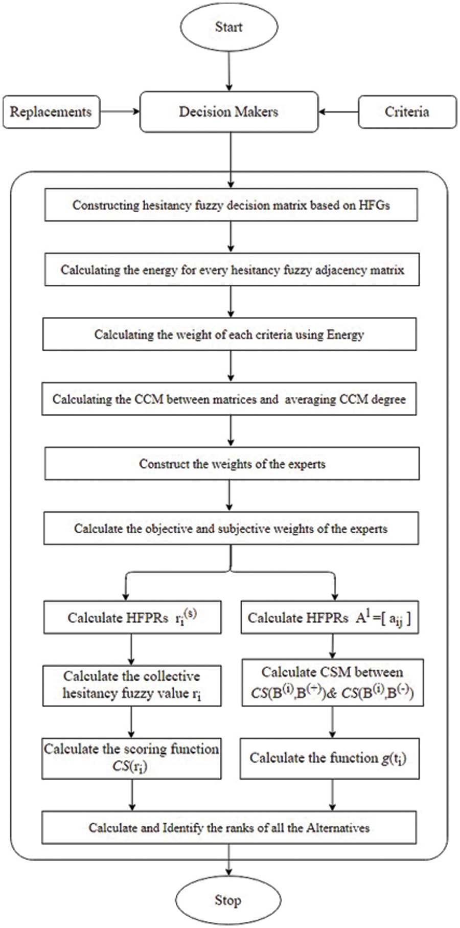
Figure 1: The measure of the correlation coefficient between hesitancy fuzzy graphs

5  Application: Choosing a Prominent Location for Electric Vehicle Charging Stations

Electric vehicles are the workhorses of today's public transportation system, offering accessible transportation to everyone. They represent a crucial first step in introducing large electric vehicles to the larger transportation industry since they are an integral part of everyday life in many cities. A piece of technology that provides electricity to EVs is known as an EV charger. Its primary function is to maintain a vehicle's mobility by recharging the battery of an EV. Due to the availability of certain smart charging stations, you may never need to visit a service station if you need to charge regularly. The main advantage of electric vehicles is the improvement in air quality they may bring to urban areas. Additionally, EVs may reduce the pollutants that contribute to pollution and environmental change, enhancing public health and minimizing ecological harm. Because there are so many different kinds of EV charging stations available, some people may find it perplexing. So, to assist you in making the best decision, below is a list of EV charging stations.

1.    Trickle charge

2.    AC charge

3.    DC charge.

Choose Trickle charge if you're EV needs a little more power to get through the day. A more moderate charge is delivered in this mode. It includes a typical three-prong, 220 V connector that is used to charge your car, making it ideal for charging smaller vehicle types. Because it is the simplest, AC charging is the most popular way to charge EVs. The charging point is directly plugged into your home's network before being connected by cable to your automobile and supplying power to the vehicle's battery. Direct current, which travels straight from the source to the car, is used by fast chargers. Fast chargers skip the converter, allowing the batteries to charge more quickly. A company wishes to launch smart charging stations for electric vehicles charging at some particular locations. This research took into account the four locations on the Dwight D. Eisenhower highway road from Denver to Kansas in the United States for launching EVCS such as A1=Strasburg,A2=Liman,A3=Flaglers,andA4=Burlington as shown in Figs. 2 and 3. Also, this research considered these locations as alternatives V={A1,A2,A3,A4} .

Figure 2: Dwight D. Eisenhower highway from Denver to Kansas in United States

Figure 3: Proposed stations from Denver to Kansas in United States

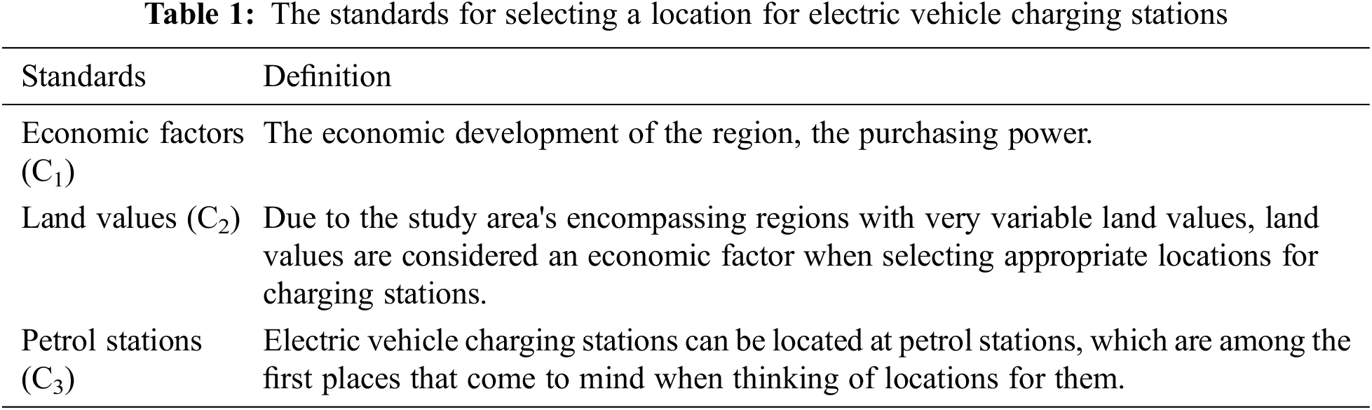
The selection of the finest location from the four alternatives for launching EVCSs is based on the criteria's as Economic Factors, Land values, Petrol stations.

Here we consider C={C1=EconomicFactors,C2=Landvalues,C3=Petrolstations} with preference information provided in the form of HFPR R=(rij) , for the particular constraints that appear in the matrices below, respectively. Suppose that in the GDM problem, there are four replacements ti,(i=1,2,3) and three experts eb,(b=1,2,and3) . Assume that the scores for every expert are 0.5 respectively and build the HFPRs as shown below. In the first place, DMs rated the language for each of the criteria based on weighted significance scores (see Table 1).

Adjacency matrix from Fig. 4

B(1)=B(HG)=[(0,0,0)(0.2,0.2,0.4)(0.3,0.4,0.2)(0.2,0.3,0.4)(0.2,0.2,0.4)(0,0,0)(0.2,0.4,0.2)(0.1,0.3,0.5)(0.3,0.4,0.2)(0.2,0.4,0.2)(0,0,0)(0.2,0.4,0.2)(0.2,0.3,0.4)(0.1,0.3,0.5)(0.2,0.4,0.2)(0,0,0)]

Figure 4: Hesitancy fuzzy preference relation for economic factors (C1)

Adjacency matrix from Fig. 5

B(2)=B(HG)=[(0,0,0)(0.2,0.5,0.2)(0.3,0.4,0.3)(0.4,0.3,0.2)(0.2,0.5,0.2)(0,0,0)(0.2,0.5,0.3)(0.1,0.6,0.2)(0.3,0.4,0.3)(0.2,0.5,0.3)(0,0,0)(0.2,0.6,0.2)(0.4,0.3,0.2)(0.1,0.6,0.2)(0.2,0.6,0.2)(0,0,0)]

Figure 5: Hesitancy fuzzy preference relation for land values (C2)

Adjacency matrix from Fig. 6

B(3)=B(HG)=[(0,0,0)(0.4,0.3,0.2)(0.2,0.4,0.3)(0.4,0.3,0.2)(0.4,0.3,0.2)(0,0,0)(0.2,0.4,0.3)(0.5,0.1,0.2)(0.2,0.4,0.3)(0.2,0.4,0.3)(0,0,0)(0.2,0.4,0.2)(0.4,0.3,0.2)(0.5,0.1,0.2)(0.2,0.4,0.2)(0,0,0)]

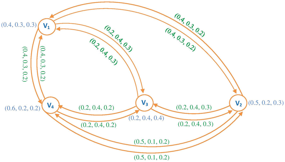
Figure 6: Hesitancy fuzzy preference relation for petrol stations (C3)

Stage I: The Energy of adjacency matrices B(1),B(2) and B(3) of HFG using Eq. (9) we get

E(B(1))=(1.2246,2.0203,1.9791)

E(B(2))=(1.2246,2.9245,1.4111)

E(B(3))=(1.9791,1.9376,1.4111).

Stage II: Calculate the scores of each expert, using Eq. (10) we get

w11=[0.2765,0.2817,0.4112]

w21=[0.2765,0.4481,0.2939]

w31=[0.4469,0.2702,0.2939].

Stage III: Calculate Karl Pearson's correlation coefficient measures CC(B(k),B(d)) between B(k) and B(d) for every k≠d , using Eq. (11) we get

CC(B(1),B(2))=2.4616

CC(B(2),B(3))=2.6329

CC(B(1),B(3))=2.6013.

From Eq. (12), to calculate the average correlation coefficients degree CC (B(k)) of B(k) is obtained as below,

CC(B(1))=2.5315

CC(B(2))=2.5473

CC(B(3))=2.6171.

Stage IV: By calculating the values of the scores wkb using Eq. (13), we get

wb=(0.3289,0.3310,0.3401)

Stage V: Compute the “objective” scores wk2 of the expert ek .

Suppose η=0.5 , which means the objective weight is affected by half of the weight determined by the CCM. The objective weighting vector can be obtained by Eq. (14), we get

w12=[0.3027,0.3053,0.3701]

w22=[0.3038,0.3896,0.3125]

w32=[0.3940,0.3052,0.3170]

Stage V: Compute the subjective and objective scores wk1 and wk2 of the expert ek .

Based on the decision-makers preferences for the objective and subjective weight vectors, Eq. (15) can integrate the subjective weighting vector w11,w21,w31 and the objective weighting vector w12,w22 , and w32 into the integrated weighting vector w1,w2 , and w3 . In Eq. (15), we assume that γ=0.5 and calculate the integrated weighting vector wk , we have

w1=[0.2896,0.2967,0.3935]

w2=[0.2896,0.4189,0.3055]

w3=[0.4174,0.2854,0.3055]

So far, we have obtained the integrated weights of experts for the practical DMP. The ranking of replacements is then determined by integrating the weighting vector w1,w2, and w3 into the HFPRs of an expert.

Firstly, we present Xu's technique for determining the decision outcome, which includes the following steps in the procedure-I:

Working Procedure-I

Stage I: Compute the average hesitancy fuzzy values (HFVs) ri(k) of replacements ti to another replacement, using Eq. (16), we have

r1(1)=(0.2333,0.3000,0.3333),r2(1)=(0.1667,0.3000,0.3667)r3(1)=(0.2333,0.4000,0.2000),r4(1)=(0.1667,0.3333,0.3667)r1(2)=(0.3000,0.4000,0.2333),r2(2)=(0.1667,0.5333,0.2333)r3(2)=(0.2333,0.5000,0.2667),r4(2)=(0.2333,0.5000,0.2000)r1(3)=(0.3333,0.3333,0.2333),r2(3)=(0.3667,0.2667,0.2333),r3(3)=(0.2000,0.4000,0.2667),r4(3)=(0.3667,0.2667,0.2000).

Stage II: By using the Eq. (17), to find all ri(k) , k is having 1,2,…,n , according to n experts, r1=(ui,vi) represents the collective hesitancy fuzzy value of replacement xi over all the other replacements, we have

r1=(0.2936,0.3517,0.2737),

r2=(0.2496,0.3885,0.2868),

r3=(0.2186,0.4423,0.2417),

r4=(0.2682,0.3845,0.2665).

Stage III: By using Eq. (18), to find the score function of ri , we get

CC(r1)=0.4040

CC(r2)=0.2721

CC(r3)=0.0328

CC(r4)=0.2793

Therefore,

CC(r1)>CC(r4)>CC(r2)>CC(r3)

And hence

v1>v4>v2>v3

where > denotes that one alternative is chosen over the other replacement.

Working Procedure-II

This research now provides the ranking result obtained using our absolute correlation coefficient approach. The collective HFPR Al=(rij)n×n is calculated using Eq. (19) in working procedure II as follows

Stage I: Compute the cooperative HFPR by using Eq. (19), we get

Al=[(0,0,0)(0.2828,0.3544,0.2796)(0.2572,0.4004,0.2620)(0.3924,0.3003,0.2796)(0.2828,0.3544,0.2796)(0,0,0)(0.2252,0.4423,0.2620)(0.2796,0.3689,0.3190)(0.2572,0.4004,0.2620)(0.2252,0.4423,0.2620)(0,0,0)(0.2252,0.4842,0.2009)(0.3924,0.3003,0.2796)(0.2796,0.3689,0.3190)(0.2252,0.4842,0.2009)(0,0,0)]

Stage II: Calculate the correlation coefficient measure CC(Bi,B+) between Bi and B+ for every replacement by using Eq. (20), we have

CC(B1,B+)=0.7988,

CC(B2,B+)=0.7472,

CC(B3,B+)=0.6427,

CC(M4,B+)=0.7488.

Stage III: Calculate the correlation coefficient measure CC(Bi,B−) between Mi and M− for every replacement by using Eq. (21), we have

CC(B1,B−)=0.4828,

CC(B2,B−)=0.5274,

CC(B3,B−)=0.5935,

CC(B4,B−)=0.5084.

Stage IV: Calculate the values of g(vi) by using Eq. (22), we get

g(v1)=0.6199

g(v2)=0.5811

g(v3)=0.5147

g(v4)=0.5866.

Now, g(v1)>g(v2)>g(v4)>g(v3) such that

v1>v4>v2>v3.

Hence v1 places in the highest position, while v3 places in the last position, and finally v4 and v2 place in the centre position order.

Therefore, according to working procedure II and Xu's technique, v1 ranks first and v3 ranks last place are, v4 and v2 have distinct ranking orders. Both techniques provide somewhat different selection orders for replacements, but the advantage of v4 over v2 , or vice versa, is not much greater than that of the other pairs of replacements, because the difference between g(v2) and g(v4) in the working procedure-II is 0.0055.

According to the preceding example, working procedure-II reasonably ranks the replacements in actual practice. Furthermore, the evaluation values of alternatives acquired by the formula in working procedure-II can also be used as weights for further analysis, but the other methods do not give this type of information because they provide HFVs or interval values rather than crisp values. Alternatively, we utilized working procedure-I to generate expert objective weights based on their HFPRs. The parameters γ can be chosen under practical conditions based on the decision-makers’ preference for subjective or objective weighted information from experts. Furthermore, by combining working procedure-I and working procedure-II, DMPs allowed for a more flexible and effective approach to HFPR.

6  Conclusion

Hesitancy fuzzy information has been used to formulate many correlation coefficient measure formulas in recent years. In this article, the correlation coefficient measures used to measure the uncertainty of HFPRs and the mean degree of correlation coefficient measures of one particular HFPR to all the others. This research present a technique for assessing the important weights of an expert that takes into consideration both the experts’ subjective and objective weights. The subjective portion of the weights referred to the conventional consequences, which are generally established by the experts’ social reputation or administrative positions in actuality. By using working procedure-I, we derive the experts’ practical judgments about the replacements and transform them into their objective weights. A hesitancy fuzzy weighted averaging operator is also used to aggregate HFPRs, which are aggregated into a collective HFPR, and a relative correlation coefficient measures method is proposed for obtaining alternative priorities from the collective HFPR by working procedure-II. This paper presented an example to demonstrate the feasibility of our methods by comparing them to some others. Also, working procedure-II can be used to derive an evaluation value of the alternatives for further analysis.

In future studies, the application of the presented technique to energy will expand to include Lapalcian energy and also needs to be examined in other practical related domains.

Acknowledgement: The authors wish to express their sincere thanks to the Vellore Institute of Technology, Vellore, Tamil Nadu, India for their financial support.

Funding Statement: This research work supported and funded was provided by Vellore Institute of Technology.

Conflicts of Interest: The authors declare that they have no conflicts of interest to report regarding the present study.

References

1. V. Torra and Y. Narukawa, “On hesitant fuzzy sets and decision,” in The 18th IEEE Int. Conf. on Fuzzy Systems, Jeju Island, Korea, pp. 1378–1382, 2009. [Google Scholar]
2. M. M. Xia and Z. S. Xu, “Hesitant fuzzy information aggregation in decision making,” International Journal of Approximate Reasoning, vol. 52, no. 3, pp. 395–407, 2011. [Google Scholar]
3. H. C. Liao and Z. S. Xu, “Subtraction and division operations over hesitant fuzzy sets,” Journal of Intelligent and Fuzzy Systems, vol. 27, no. 1, pp. 65–72, 2014. [Google Scholar]
4. V. Torra, “Hesitant fuzzy sets,” International Journal of Intelligent Systems, vol. 25, no. 6, pp. 529–539, 2010. [Google Scholar]
5. H. C. Liao and Z. S. Xu, “Some new hybrid weighted aggregation operators under hesitant fuzzy multi-criteria decision making environment,” Journal of Intelligent and Fuzzy Systems, vol. 26, no. 4, pp. 1601–1617, 2014. [Google Scholar]
6. H. C. Liao and Z. S. Xu, “Extended hesitant fuzzy hybrid weighted aggregation operators and their application in decision making,” Soft Computing, vol. 19, no. 9, pp. 2551–2564, 2015. [Google Scholar]
7. H. C. Liao, Z. S. Xu and J. P. Xu, “An approach to hesitant fuzzy multi-stage multi-criterion decision making,” Kybernetes, vol. 43, pp. 1447–1468, 2014. [Google Scholar]
8. H. C. Liao, Z. S. Xu and M. M. Xia, “Multiplicative consistency of hesitant fuzzy preference relation and its application in group decision making,” International Journal Information Technology and Decision Making, vol. 13, no. 1, pp. 47–76, 2014. [Google Scholar]
9. B. Zhu and Z. S. Xu, “Deriving a ranking from hesitant fuzzy preference relations under group decision making,” IEEE Transactions on Cybernetics, vol. 44, no. 8, pp. 1328–1337, 2013. [Google Scholar]
10. H. C. Liao and Z. S. Xu, “A VIKOR-based method for hesitant fuzzy multi-criteria decision making,” Fuzzy Optimization and Decision Making, vol. 12, no. 4, pp. 373–392, 2013. [Google Scholar]
11. Z. S. Xu and X. L. Zhang, “Hesitant fuzzy multi-attribute decision making based on TOPSIS with incomplete weight information,” Knowledge-Based Systems, vol. 52, pp. 53–64, 2013. [Google Scholar]
12. X. L. Zhang and Z. S. Xu, “The TODIM analysis approach based on novel measured functions under hesitant fuzzy environment,” Knowledge-Based Systems, vol. 61, pp. 48–58, 2014. [Google Scholar]
13. H. C. Liao and Z. S. Xu, “Satisfaction degree based interactive decision making method under hesitant fuzzy environment with incomplete weights,” International Journal of Uncertainty, Fuzziness and Knowledge-Based Systems, vol. 22, no. 4, pp. 553–572, 2014. [Google Scholar]
14. C. A. Murithy, S. K. Pal and D. Dutta-Majumder, “Correlation between two fuzzy membership functions,” Fuzzy Sets and Systems, vol. 17, no. 1, pp. 23–38, 1985. [Google Scholar]
15. B. B. Chaudhuri and A. Bhattacharya, “On correlation between two fuzzy sets,” Fuzzy Sets and Systems, vol. 118, no. 3, pp. 447–456, 2001. [Google Scholar]
16. D. A. Chiang and N. P. Lin, “Correlation of fuzzy sets,” Fuzzy Sets and Systems, vol. 102, no. 2, pp. 221–226, 1999. [Google Scholar]
17. C. H. Yu, “Correlation of fuzzy numbers,” Fuzzy Sets and Systems, vol. 55, no. 3, pp. 303–307, 1993. [Google Scholar]
18. S. T. Liu and C. Kao, “Fuzzy measures for correlation coefficient of fuzzy numbers,” Fuzzy Sets and Systems, vol. 128, no. 2, pp. 267–275, 2002. [Google Scholar]
19. D. H. Hong, “Fuzzy measures for a correlation coefficient of fuzzy numbers under T w (the weakest t-norm)-based fuzzy arithmetic operations,” Information Sciences, vol. 176, no. 2, pp. 150–160, 2006. [Google Scholar]
20. Z. S. Xu and M. M. Xia, “On distance and correlation measures of hesitant fuzzy information,” International Journal of Intelligent Systems, vol. 26, no. 5, pp. 410–425, 2011. [Google Scholar]
21. N. Chen, Z. S. Xu and M. M. Xia, “Correlation coefficients of hesitant fuzzy sets and their application to clustering analysis,” Applied Mathematical Modelling, vol. 37, no. 4, pp. 2197–2211, 2013. [Google Scholar]
22. W. L. Hung, “Using statistical viewpoint in developing correlation of intuitionistic fuzzy sets,” International Journal of Uncertainty, Fuzziness and Knowledge-Based Systems, vol. 9, no. 4, pp. 509–516, 2001. [Google Scholar]
23. E. Szmidt and J. Kacprzyk, “Correlation of intuitionistic fuzzy sets,” in Proc. Int. Conf. on Information Processing and Management of Uncertainty in Knowledge-Based Systems, Berlin, Heidelberg, pp. 169–177, 2010. [Google Scholar]
24. H. B. Mitchell, “A correlation coefficient for intuitionistic fuzzy sets,” International Journal of Intelligent Systems, vol. 19, no. 5, pp. 483–490, 2004. [Google Scholar]
25. T. Gerstenkorn and J. Manko, “Correlation of intuitionistic fuzzy sets,” Fuzzy Sets and Systems, vol. 44, no. 1, pp. 39–43, 1991. [Google Scholar]
26. D. H. Hong and S. Y. Hwang, “Correlation of intuitionistic fuzzy sets in probability spaces,” Fuzzy Sets and Systems, vol. 75, no. 1, pp. 77–81, 1995. [Google Scholar]
27. W. L. Hung and J. W. Wu, “Correlation of intuitionistic fuzzy sets by centroid method,” Information Sciences, vol. 144, no. 1–4, pp. 219–225, 2002. [Google Scholar]
28. Z. S. Xu, “On correlation measures of intuitionistic fuzzy sets,” in Int. Conf. on Intelligent Data Engineering and Automated Learning, Berlin, Heidelberg, pp. 16–24, 2006. [Google Scholar]
29. Z. S. Xu and M. M. Xia, “Hesitant fuzzy entropy and cross-entropy and their use in multiattribute decision-making,” International Journal of Intelligent Systems, vol. 27, no. 9, pp. 799–822, 2012. [Google Scholar]
30. Z. S. Xu and M. M. Xia, “Distance and similarity measures for hesitant fuzzy sets,” Information Sciences, vol. 181, no. 11, pp. 2128–2138, 2011. [Google Scholar]
31. B. Farhadinia, “Information measures for hesitant fuzzy sets and interval-valued hesitant fuzzy sets,” Information Sciences, vol. 240, no. 10, pp. 129–144, 2013. [Google Scholar]
32. J. H. Hu, X. L. Zhang, X. H. Chen and Y. M. Liu, “Hesitant fuzzy information measures and their applications in multi-criteria decision making,” International Journal of Systems Science, vol. 47, no. 1, pp. 62–76, 2015. [Google Scholar]
33. D. Q. Li, W. Y. Zeng and Y. B. Zhao, “Note on distance measure of hesitant fuzzy sets,” Information Sciences, vol. 321, pp. 103–115, 2015. [Google Scholar]
34. J. J. Peng, J. Q. Wang and X. H. Wu, “Novel multi-criteria decision-making approaches based on hesitant fuzzy sets and prospect theory,” International Journal of Information Technology & Decision Making, vol. 15, no. 3, pp. 621–643, 2016. [Google Scholar]
35. X. D. Liu, Z. W. Wang and A. Hetzler, “HFMADM method based on nondimensionalization and its application in the evaluation of inclusive growth,” Journal of Business Economics and Management, vol. 18, no. 4, pp. 726–744, 2017. [Google Scholar]
36. H. Garg, “A novel correlation coefficients between pythagorean fuzzy sets and its applications to decision-making processes,” International Journal of Intelligent Systems, vol. 31, no. 12, pp. 1234–1252, 2016. [Google Scholar]
37. H. Garg and D. Rani, “A robust correlation coefficient measure of complex intuitionistic fuzzy sets and their applications in decision-making,” Applied Intelligence, vol. 49, no. 2, pp. 496–512, 2019. [Google Scholar]
38. H. Garg and K. Kumar, “A novel correlation coefficient of intuitionistic fuzzy sets based on the connection number of set pair analysis and its application,” Scientia Iranica E, vol. 25, no. 4, pp. 2373–2388, 2018. [Google Scholar]
39. N. Chen, Z. Xu and M. Xia, “Correlation coefficients of hesitant fuzzy sets and their applications to clustering analysis,” Applied Mathematical Modelling, vol. 37, no. 4, pp. 2197–2211, 2013. [Google Scholar]
40. F. Meng and X. Chen, “Correlation coefficients of hesitant fuzzy sets and their application based on fuzzy measures,” Cognitive Computation, vol. 7, no. 4, pp. 445–463, 2015. [Google Scholar]
41. X. Liu, Z. Wang, S. Zhang and H. Garg, “Novel correlation coefficient between hesitant fuzzy sets with application to medical diagnosis,” Expert Systems with Applications, vol. 183, pp. 115393, 2021. [Google Scholar]
42. T. Pathinathan, J. J. Arockiaraj and J. J. Rosline, “Hesitancy fuzzy graphs,” Indian Journal of Science and Technology, vol. 8, no. 35, pp. 1–5, 2015. [Google Scholar]
43. M. Akram and G. Shahzadi, “Operation on single-valued neutrosophic graphs,” Journal of Uncertainty Systems, vol. 11, no. 3, pp. 176–196, 2017. [Google Scholar]
44. S. Broumi, M. Talea, A. Bakali and F. Smarandache, “Single valued neutrosophic graphs,” Journal of New Theory, vol. 10, pp. 86–101, 2016. [Google Scholar]
45. F. Karaaslan and B. Davvaz, “Properties of single-valued neutrosophic graphs,” Journal of Intelligent and Fuzzy Systems, vol. 34, no. 1, pp. 57–79, 2018. [Google Scholar]
46. F. Karaaslan, “Hesitant fuzzy graphs and their applications in decision making,” Journal of Intelligent and Fuzzy Systems, vol. 36, no. 3, pp. 2729–2741, 2019. [Google Scholar]
47. M. Grabisch, “Fuzzy integral in multicriteria decision making,” Fuzzy Sets and Systems, vol. 69, no. 3, pp. 279–298, 1995. [Google Scholar]
48. N. R. Reddy, M. Z. Khan, S. Sharief Basha, A. Alahmadi and A. H. Alahmadi, “The Laplacian energy of hesitancy fuzzy graphs in decision-making problems,” Computer Systems Science and Engineering, vol. 44, no. 3, pp. 2637–2653, 2023. [Google Scholar]
49. S. Guo and H. Zhao, “Optimal site selection of electric vehicle charging station by using fuzzy TOPSIS based on sustainability perspective,” Applied Energy, vol. 158, no. 15, pp. 390–402, 2015. [Google Scholar]
50. N. Shahraki, H. Cai, M. Turkay and M. Xu, “Optimal locations of electric public charging stations using real world vehicle travel patterns,” Transportation Research Part D: Transport and Environment, vol. 41, pp. 165–176, 2015. [Google Scholar]
51. W. Tu, Q. Li, Z. Fang, S. L. Shaw and B. Zhou, “Optimizing the locations of electric taxi charging stations: A spatial–temporal demand coverage approach,” Transportation Research Part C: Emerging Technologies, vol. 65, pp. 172–189, 2016. [Google Scholar]
52. S. Y. He, Y. H. Kuo and D. Wu, “Incorporating institutional and spatial factors in the selection of the optimal locations of public electric vehicle charging facilities: A case study of Beijing, China,” Transportation Research Part C: Emerging Technologies, vol. 67, pp. 131–148, 2016. [Google Scholar]
53. H. C. Liu, M. Yang, M. C. Zhou and G. Tian, “An integrated multi-criteria decision making approach to location planning of electric vehicle charging stations,” IEEE Transactions on Intelligent Transportation Systems, vol. 20, no. 1, pp. 362–373, 2018. [Google Scholar]
54. R. Ren, H. Lio, A. A. Barakati and F. Cavallaro, “Electric vehicle charging station site selection by an integrated hesitant fuzzy SWARA-WASPAS method,” Transformations in Business and Economics, vol. 18, no. 2, pp. 103–123, 2019. [Google Scholar]
55. G. Wei, C. Wei, J. Wu and Y. Guo, “Probabilistic linguistic multiple attribute group decision making for location planning of electric vehicle charging stations based on the generalized dice similarity measures,” Artificial Intelligence Review, vol. 54, no. 6, pp. 4137–4167, 2021. [Google Scholar]
Cite This Article
Copyright © 2023 The Author(s). Published by Tech Science Press.
This work is licensed under a Creative Commons Attribution 4.0 International License , which permits unrestricted use, distribution, and reproduction in any medium, provided the original work is properly cited.
Downloads
Citation Tools