Optimized Model Based Controller with Model Plant Mismatch for NMP Mitigation in Boost Converter

Nomenclature

1  Introduction

Boost converters are used as the front part of converters in solar photovoltaic systems, battery sources, and fuel cells that have a higher level of voltage output than the supply voltage. Generally boost converters are provided with closed-loop control because open-loop mode has imperfect voltage control and inefficient dynamic responsiveness. In frequency domain analysis, the location of RHPZ is in inverse relationship with the average inductor current. As a result, the increment of inductor current pushes the zero towards low frequency, which, in turn, limits the availability of bandwidth for a stable operation of the dc-dc boost converter.

Freudenberg et al. [1] discussed the hindrance of RHP poles and zeros in terms of integral relationship which will disturb the magnitude of sensitivity and interrelated functions of closed loop system. Sable et al. [2] proposed leading edge modulation with Pulse Width Modulation (PWM) to transfer the RHP zero to a stable region. However, this method requires a minimum erythrocyte sedimentation rate (ESR) time constant at the output capacitor to get better stability and ripple voltage filtering has not been done in the compensatory part. Due to the complex behavior of RHP zero, designers are forced to restrict the entire operating bandwidth to 1/30 of the switching frequency. Leyva-Ramos et al. [3] discussed the quality factor (Q) of the boost converter related to RHP zero in the design of the inner current loop. The Q value will increase when RHP zero is kept away from the poles during the voltage loop which produces undesirable effects on regulator stability. But the perception of current gain has not been thoroughly designed and complete inner and outer loop control was not presented. Alvarez-Ramirez et al. [4] discussed the design of novel gain parameterization for a PI controller with a high inductor value (L = 43.5 mH) to reduce the ripple in load current. However, the design procedure is complex, and transient analysis of RHP zero was not discussed.

Over the period, several research activities have been carried out to address the issue of RHP zero in boost converter. Chen et al. [5] have presented closed-loop cascade control of a non-minimum phase (NMP) boost converter. Huang et al. [6] proposed a solid-duty-control technique to reduce the effect of RHPZ and transient response improvement, but it is quite complex to implement. Time multiplexing current balance technique for mitigating RHP zero effect was discussed in Luo et al. [7]. This technique required an extra inductor to operate in interleaved mode and efficiency was not discussed.

The performance of the boost converter largely depends on the gain of the PID controller employed in the feedback path. More research work has been carried out in tuning PID controller parameters over the decade. The relationship between the duty ratio and voltage conversion of the boost converter is severely non-linear and therefore its performance largely depends on the gain of the PID controller employed in the feedback path [8–19]. Guo et al. [20] have proposed a fuzzy controller based on an intuitive understanding of the converter function and tweaking takes some experience to eliminate ineffective experimentation. An evolutionary algorithm-based PID parameter tuning was proposed by Sundareswaran et al. [21] with the maturation of the queen bee in a hive. However, the challenging RHPZ problems remained. This paper proposes an optimized GA for IMC–PID tuning parameters which gives better-computed results in terms of servo and regulatory responses and the results were compared with conventional IMC-PID and Zeigler Nichols (ZN) PID parameter responses. To build a robust controller structure, the small signal model of a boost converter is used to evaluate the GA’s objective function.

This paper is organized as follows: Small signal analysis of the proposed boost converter and its open-loop study with a negative dip in output response due to the boost inductor is discussed in Section 2. In Section 3, dynamic controller design issues due to RHPZ are narrated as a problem statement. Sections 4 and 5 deal with conventional IMC–PID and GA–IMC PID structure and their performances in the closed-loop analysis is explained in Section 6 followed by a conclusion.

2  Averaged Small Signal Model of DC–DC Boost Converter

The first step of this paper is to develop a transfer function model for proposed non-linear variable structure systems. The schematic of an analogous boost converter circuit is shown in Fig. 1.

Figure 1: Equivalent circuit of boost converter

The state and output equation of boost behavior at the switch ON position will be given by

[iLb˙νCb˙]=[−rLbLb00−1(Ro+rCb)Cb][iLbνCb]+[1Lb0][νg](1)

νo=[0Ro(Ro+rCb)Lb][iLbνCb](2)

Similarly, the state and output equation of boost behavior at the switch OFF position will be given by

[iLb˙νCb˙]=[−RorCb(Ro+rCb)Lb−RoLb(Ro+rCb)Ro(Ro+rCb)Cb−1Cb(R0+rCb)][iLbνCb]+[1Lb0][νg](3)

νo=[RorCbRo+rCbRo(R0+rCb)Cb][iLbνCb](4)

Since the above-mentioned system is non-autonomous, the state space representation is in discontinuous mode. The idea of the averaging method is to approximate the system behavior. Here the matrices A, B, and C are being weighted by ‘d’ (duty ratio), by the fact that ‘d’ keeps on changing concerning time. Therefore the large signal model is non-linear because it has time-varying matrices due to the switches involved. Most of the time the system is going to be in a steady state (equilibrium) for a large portion of time, therefore, the design of the plant using the steady state equation is very important. Subtracting the steady state part from the large signal part gives a small signal model which provides an idea of the dynamics of the converter about its operating point.

Small signal transfer function describes the effect of control input d(s) on output voltage vo(s) with initial conditions (vgs = 0 & ios = 0) is used in this controller design of boost converter is given.

Gp(s)=νo(s)d(s)=Vg(1−D)2[(1+sCbrCb)(1−Lb(1−D)2Ros)(LbCb(Ro+rCb)(1−D)2Ro+rLb)s2+(Lb(1−D)2Ro+rCbCb)s+1](5)

Therefore Gp(s) decides the loop gain and has a significant effect on the servo and regulator performance. Here the disturbances are variation in input voltage with respect to output voltage (d(s)=0&io(s)=0) and change in load current with respect to output voltage (vg(s)=0&d(s)=0) are given below

Gd1(s)=νo(s)νg(s)=[(1+sCbrCb)(1−D)Ro(Ro+rCb)(LbCb(R0+rCb)(1−D)2Ro+rLb)s2+(Lb(1−D)2Ro+rCbCb)s+1](6)

Gd2(s)=−νo(s)io(s)=−[(1+sCbrCb)Ro×[Ro(1−D)rCb−Ro(1−D)2rCb+(Ro+rCb)Lbs](LbCb(Ro+rCb)(1−D)2Ro+rLb)s2+(Lb(1−D)2Ro+rCbCb)s+1](7)

To study the dynamic behavior of the dc-dc boost converter, its control variable to output variable transfer function (5) can be modified as

Gp(s)=νo(s)d(s)=Kp(1+αs)(1−βs)((τ1s+1)(τ2s+1))(8)

The above-mentioned transfer function Gp(s) has a steady state process gain Kp, two poles (P1 = −1/τ1 & P2 = −1/τ2), RHPZ at Z1 = 1/β (yielding inverse response), and ESRZ. For this discussion, the ESRZ (1 + αs) will be ignored because it is at a much higher frequency than the double-pole frequency and RHPZ. On substituting the values of the boost converter listed in Table 1., the Eqs. (5)–(7) becomes

Gp(s)=75(1−0.02447s)0.000029286s2+0.02451s+1(9)

Gd1(s)=60(1+0.00004s)0.000029286s2+0.02451s+1(10)

Gd2(s)=−13.8(1+0.00004s)(1+0.5059s)0.000029286s2+0.02451s+1(11)

To study the effects of RHPZ on converter stability, the closed loop characteristic equation of boost converter with proportional control Gc(s)=Kc is considered and given by

1+Gc(s)Gp(s)=1+Gol(s)=1+KcKp(1−βs)((τ1s+1)(τ2s+1))=0(12)

Replacing K=KcKp then the above Eq. (12) becomes,

1+K(1−βs)((τ1s+1)(τ2s+1))=0(13)

The root locus of open loop transfer function Gol(s) for varying values of K with fixed Kp is shown in Fig. 2. The presence of RHPZ limits the ultimate gain K=Ku=0.99 at crossover frequency ωc = 227 rad/sec, above which the converter becomes unstable and corresponding proportional controller gain is called as ultimate controller gain Kcu and it is found to be 0.0132.

Figure 2: Root locus of open loop transfer function

Fig. 3 depicts the boost converter’s open-loop step response which begins with a negative slope and reaches a negative maximum of −60 V, which is over 80% of the eventual steady-state output value of 75 V. Subsequently the response takes almost one time constant τ2 (20 msec) to come back to zero. Due to the existence of the boost inductor, L, the percentage undershoot is directly proportional to β, which is known as inverse response and it occurs in the boost converter. This results in an RHPZ, which limits the closed-loop bandwidth and hence the controller gain nKc.

Figure 3: Open loop step response

3  RHPZ Issue in Dynamic Controller Design

The usage of dynamic control law can help to speed up the response time of a system. The relationship between reference input r(s) and output y(s) from Fig. 4 will be given by,

Figure 4: Model-based open loop control system

y(s)=Gp(s)q(s)r(s)=Gp(s)1Gp(s)r(s)=r(s)(14)

where q(s)=1Gp(s) ; model based controller.

From (14) it is shown that the output perfectly tracks the set point. In a practical situation, a proper controller should be employed with the help of the process model inverse, coupled with a filter transfer function. For better control, controller q(s), should be dynamic rather than static.

On considering the dc-dc boost converter transfer function having RHPZ at 40.8 min−1 (1/β)

Gp(s)=νo(s)d(s)=75(1−0.02447s)(0.000029286s2+0.02451s+1)(15)

Dynamic open loop controller can be given by

q(s)=Gp−1(s)f(s)=(0.000029286s2+0.02451s+1)75(1−0.02447s)f(s)(16)

where f(s)=1/(λs+1), filter transfer function.

When the model inverse is employed to construct a control system, the zeros of the process model become the pole of the controller, resulting in an unstable controller. As a result, before employing the model inverse for controller design, RHPZ must be factored out from the process.

Case (i) when the unstable controller pole is removed

If the unstable pole is simply taken from (16), then

q(s)=Gp−1(s)f(s)=(0.000029286s2+0.02451s+1)75(λs+1)(17)

But (17) is invalid due to improper q(s). To design a proper controller, the order of the filter can be increased. Therefore (17) becomes,

q(s)=Gp−1(s)f(s)=(0.000029286s2+0.02451s+1)75(λs+1)(λs+1)(18)

The resulting manipulated and output variable response will be

u(s)=(0.000029286s2+0.02451s+1)75(λs+1)(λs+1)r(s)(19)

y(s)=(1−0.02447s)(λs+1)(λs+1)r(s)(20)

The manipulated variable and output responses of the case (i) for a unit step change in set point are shown in Fig. 5 for various filter tuning settings (λ). It’s worth noting that when the set point is changed, the manipulated input changes instantly, and the output variable shows an inverse response. As a result, no stability control system can eliminate the process inverse response behavior.

Figure 5: Unit step response with stable controller

Case (ii) when the unstable controller pole is not removed

If the unstable pole is not removed from (16), then (21) represents an unstable controller.

q(s)=(0.000029286s2+0.02451s+1)75(1−0.02447s)(λs+1)(21)

The resulting manipulated variable response and output response will be

u(s)=(0.000029286s2+0.02451s+1)75(1−0.02447s)(λs+1)r(s)(22)

y(s)=1(λs+1)r(s)(23)

The manipulated variable and output responses of the case (ii) for a unit step change in set point are shown in Fig. 6. for various filter tuning settings (λ). The output variable does not contain the inverse response, but the manipulated variable is indefinite. This scenario is referred to as internal instability. To suppress the internal stability issues in open loop unstable processes, it is required to apply the internal model control (IMC) mechanism in the standard feedback form. Hence, open-loop stable systems are taken into account in this paper [22,23].

Figure 6: Unit step response with unstable controller

4  Internal Model Control

According to the literature study, most of the available approaches incorporate the conventional feedback mechanism to handle the boost converter operation. But the internal model control (IMC) structure provides a transparent framework to deal with model uncertainty. The advantages of this technique over conventional feedback structure are bolstered by the fact that set point tracking and disturbance rejection can be set by a single filter tuning parameter (λ).

A mismatch between actual plant Gp(s) and model plant Gm(s) occurs due to the changes in operating conditions and linearization of errors. Studies reported assumed that there is no mismatch between the model and plant. In practice, however, having a perfect model of the plant is usually a challenging task. For extremely non-linear processes, the process gain can sometimes be off by 20–50 percent or even more. While designing the controller, the designer assumed the real plant is equal to the model plant. In practice, they are often different, and the controller needs to be robust enough to track set points and reject disturbances. As a result, while open-loop control cannot adapt to disturbances or model uncertainty, IMC can. The conventional feedback scheme and IMC structure are shown in Figs. 7 and 8 respectively.

Figure 7: Conventional feedback control scheme

Figure 8: Internal model control (IMC) scheme

In IMC, the process model is parallel to the actual process; therefore the discrepancy between model predictions and measured signal contains direct information on model-plant mismatch and unmeasured disruptions. Thus IMC is fundamentally a predictive control scheme.

Algorithm for Conventional IMC-PID Design

Step 1: Servo response can be shaped by the inverse of the linear perturbation model in IMC design. But, for an NMP system, the usage of model inverse in controller design results in a physically unrealizable controller which was explained in Section 3. To overcome this issue, factorization of the process model into the invertible part (the good part), Gm−(s), and non-invertible part (bad part), Gm + (s) is done. In this paper, (Gps ≠ Gms) case is considered where the real-world problem exists. Here the model plant Gm(s) is different from the process plant Gp(s) by two times of increased gain and 20% of increased time constant as shown in the below equation. Eq. (24) is different from Eq. (15) by the above-said parameters.

Gm(s)=Gm+(s)Gm−(s)=150(1−0.02447s)0.00004218s2+0.02941s+1(24)

Step 2: Inversing the invertible portion of the model plant (after all pass factorization) is the ideal internal model controller.

q~(s)=Gm−−1(s)=(0.00004218s2+0.02941s+1)150(1+0.02447s)(25)

Step 3: To make the controller proper, a filter is added

q(s)=q~(s)f(s)=(0.00004218s2+0.02941s+1)150(1+0.02447s)1(λs+1)(26)

The filter transfer function f(s)=1(λs+1)n is ideal to track reference changes and ‘n’ is selected to keep the controller proper/semi-proper. To supress the disturbances, a filter f(s)=(Υs+1)(λs+1)n will often are used, where ‘ϒ’ is selected to supress the slow process time constant. This procedure brings down the Eq. (14) into the following forms

y(s)=(1+0.02447s)(1−0.02447s)(λs+1)r(s)(27)

y(s)=G1(s)r(s)+G2(s)d(s)(28)

where,

G1(s)=(75(1−0.02447s)(0.000029286s2+0.02451s+1)∗(0.00004218s2+0.02941s+1)150(1+0.02447s)(λs+1)1+(0.00004218s2+0.02941s+1)150(1+0.02447s)(λs+1)(75(1−0.02447s)(0.000029286s2+0.02451s+1)−150(1−0.02447s)0.00004218s2+0.02941s+1))

G2(s)=(1−(150(1−0.02447s)(0.00004218s2+0.02941s+1)∗(0.00004218s2+0.02941s+1)150(1+0.02447s)(λs+1))1+(0.00004218s2+0.02941s+1)150(1+0.02447s)(λs+1)(75(1−0.02447s)(0.000029286s2+0.02451s+1)−150(1−0.02447s)0.00004218s2+0.02941s+1))

Eq. (27) represents perfect model case (no model mismatch) with no disturbances: (Gp(s)=Gm(s)) & Gd(s)=0 whereas, (28) represents model uncertainty (model mismatch) case with disturbances: (Gp(s)≠Gm(s)) & Gd(s)≠0. In Eq. (28), if the model is equal to the process and there is no disturbance, then (28) will behave like (27). Therefore non-minimum phase component must appear in the output response even in perfect model conditions. The design of the internal model controller depends on the technique used for factorizing the model. Output responses of different controller factorizations will be given by

Simple Factorization:

y(s)=(1−βs)(λs+1)2r(s)(29)

This equation is referred as complementary sensitivity function in case of integral absolute error (IAE) =∫0Ts|Vo,ref(s)−Vo(s)|dt, where Ts is settling time.

All–Pass Factorization:

y(s)=(1−βs)(βs+1)(λs+1)r(s)(30)

This equation is referred to as a complementary sensitivity function in case of integral square error (ISE) = ∫0Ts(Vo,ref(s)−Vo(s))2dt, where Ts is the settling time which is different from (29). By analyzing the error performance criteria of IAE and ISE for the proposed converter in this paper, it was observed that the integral square error value dominates the performance measure shown in Fig. 9. The corresponding IAE and ISE values are listed in Table 2. Therefore minimizing ISE will be an objective function of this proposed control system and all pass factorization is used, because the resulting control system minimizes the integral square error (ISE).

Figure 9: Error performance evaluation of input voltage variation, load variation, and set point tracking

Up to step 3, the procedure follows the IMC structure. But there is a major difference in finding the equivalent form of PID controller from IMC. The equivalent feedback form to IMC is shown in Fig. 10.

Figure 10: Standard feedback with equivalent IMC

Step 4: Controller parameter evaluation using the equivalent standard feedback form

Gc(s)=q(s)1−Gm(s)q(s)=(0.00004218s2+0.02941s+1)150(0.02447λs2+(0.04894+λ)s)(31)

The transfer function of the ideal PID controller is given by,

Gc(s)=Kc[τIτDs2+τIs+1τIs](32)

On rearranging the Eq. (31) with the ideal PID form (32), the filter tuning parameter λ and PID controller parameters can be obtained.

Kc=2ζτKp(2β+λ);τI=2ζτ;τD=τ2ζ;τF=βλ2β+λ(33)

Step 5:

After calculating Kc, τI, τD, PID controller cascaded with first order filter is created.

Gc(s)=Kc[τIτDs2+τIs+1τIs][1τFs+1](34)

Thumb Rule: Initial values of λ will generally be around 1/3 to 1/2 the dominant time constant and λ > β/2 to suppress the dominant time constant.

5  Genetic Algorithm

Genetic Algorithm (GA) is a probabilistic random search method, used to solve non-linear systems and optimize complex problems. This approach begins by initializing a population of individuals in random manner to evaluate the objective function. In this paper, the GA evaluates the gains of IMC PID control as system gain (Kp,KI,KD,λ) in order to minimize the cost function given by the following integral square error performance criterion, ISE = ∫0Ts(Vo,ref(s)−Vo(s))2dt, where Ts is settling time.

Algorithm for GA-based IMC–PID Design

The controller design has now been transformed into an optimization problem, as seen below.

MinimizeF(Φ)=∑t=0Ts⁡(Vo,ref(s)−Vo(s))2;Φlower≤Φ≤Φupper(35)

The steps below illustrate how a GA is developed and applied to the current problem.

Step 1: Initialization of population

Genetic algorithm steps initiated with the creation of an initial population for parameters (Kp,KI,KD,λ) with population size. It is well established in the literature that a population size of 10–30 is appropriate; the population size in this study is set at 20. A gene is a term used to describe each variable in the problem.

Each chromosome represents a solution to the problem because it is made up of genes. A set of chromosomes makes up the population. The ISE value calculated from Eq. (30) is used to determine the fitness of each chromosome. The parameter range for controller gain and tuning filter is given as (z (1) represents zeros (1) and o (1) represents ones (1)),

KP∈[0,100]; {minx(1)=z(1);maxx(1)=100∗o(1)}

KI∈[0,75] ; {minx(2)=z(1);maxx(2)=75∗o(1)}

KD∈[0,75] ; {minx(3)=z(1);maxx(3)=75∗o(1)}

λ∈[0,5] ; {minx(4)=z(1);maxx(4)=5∗o(1)}

Step 2: Evaluation of objective function

Eqs. (2) and (4) are used to evaluate Vo(s) for a given chromosome, then the value of F(Φ) is computed for each chromosome.

Step 3: Evaluation of Fitness Function

The perfection of the solution is evaluated by defining a proper fitness function for the problem. Because of the minimization objective function, a chromosome with a low fitness value has a high likelihood of becoming fit.

Step 4: Generation of offspring

Selection, crossover, and mutation produce offspring, which are new chromosomes. After calculating the fitness of each chromosome, parent solutions are chosen for reproduction. It mimics nature’s survival of the fittest method.

Step 5: To build up the new cluster, replace the present population with the new one.

Step 6: If the termination requirement is met, exit the program; otherwise, go to Step 2.

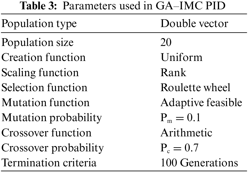
Table 3 shows the parameters used in GA–IMC PID.

6  Objectives of Closed Loop System

The primary concern of a closed loop system is to be immune to external disturbances and track the desired set point. From the control point of view, the external voltage source vg(t) and load current io(t) represent the disturbance inputs whereas the controlled variable is vo(t). The objective functions of a closed loop system are verified by the conventional Zeigler-Nichols PID tuning method, conventional IMC-PID method, and genetic algorithm-tuned IMC-PID methods. The above-said controller methods are compared based on the following indices (i) Settling time and (ii) Percentage overshoot/undershoot. The values of PID parameters and filter tuning parameters of the above-said methods are given in below Table 4.

Servo Response: Tracking the desired set-point voltage

In this example, set-point tracking and disturbance rejection was analyzed. The comparison of controller performance based on settling time is shown in Table 5 (ms). Comparing controller performance based on peak overshoot/undershoot (%) is shown in Table 6.

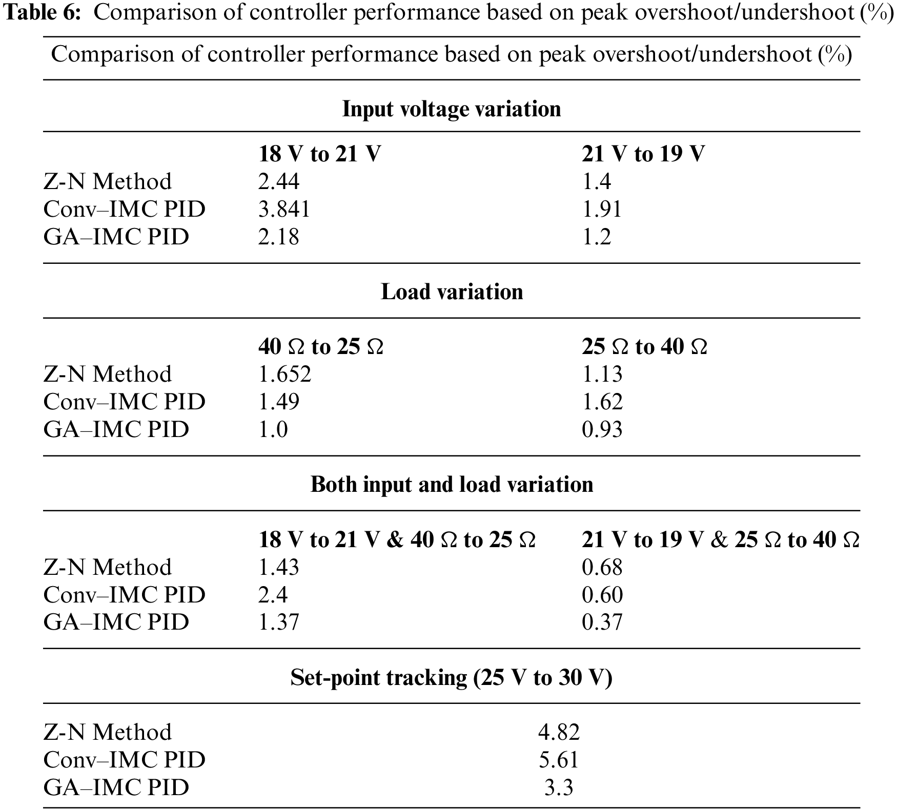
Fig. 11 displays the reactions of set point tracking and disruption. Rejection results in the absence of model mismatch, gain mismatch, and process time constant.

Figure 11: (a) Set point tracking performance; (b) Disturbance rejection performance (No model mismatch: Gp(s) = Gm(s); Mismatch in time constant: 20% of increased τ; Mismatch in gain: New gain =2 * Kp)

7  Conclusion

The output voltage control of a boost-type dc-dc converter working in continuous conduction mode with non-minimum phase dynamics is handled in this study by an optimized evolutionary algorithm-based IMC-PID. A better base for controller tuning is provided by the IMC structure with ISE factorization for minimization of error. GA-IMC PID outperforms conventional model control and ZN-PID from a control perspective in terms of both performance indices (settling point and overshoot/undershoot). The computed outcomes successfully demonstrated the IMC PID controller’s robustness under the conditions of model plant mismatch. The fact that GA-tuned IMC PID directly manipulates the switches without the use of a modulator is one of its main advantages. The GA-tuned IMC PID’s incorporation of current limitations, which do not require the usage of an additional current loop, is an additional benefit. Less overshoot/undershoot, a shorter response time, and an inherent feed forward are further positive features of the proposed GA-tuned IMC PID. The computational complexity of GA-tuned IMC PID is typically a downside. Nevertheless, the converter is minimum phase, allowing for the use of a modest value of the prediction horizon, which lowers the computational cost.

Funding Statement: The authors received no specific funding for this study.

Conflicts of Interest: The authors declare that they have no conflicts of interest to report regarding the present study.

References

    1. S. J. Freudenberg and P. D. Looze, “Right half plane poles and zeros and design trade-offs in feedback systems,” IEEE Transactions on Automatic Control, vol. 30, no. 6, pp. 555–565, 1985. [Google Scholar]

    2. M. D. Sable, H. B. Cho and B. R. Ridley, “Use of leading-edge modulation to transform boost and flyback converters into minimum-phase-zero systems,” IEEE Transactions on Power Electronics, vol. 6, no. 4, pp. 704–711, 1991. [Google Scholar]

    3. J. Leyva-Ramos and J. A. Morales-Saldana, “A design criteria for the current gain in current-programmed regulators,” IEEE Transactions on Industrial Electronics, vol. 45, no. 4, pp. 568–573,1998, 1998. [Google Scholar]

    4. J. Alvarez-Ramirez, I. Cervantes, G. Espinosa-Perez, P. Maya and A. Morales, “A stable design of PI control for DC-DC converters with an RHS zero,” IEEE Transactions on Circuits and Systems I: Fundamental Theory and Applications, vol. 48, no. 1, pp. 103–106, 2001. [Google Scholar]

    5. Z. Chen, W. Gao, J. Hu and X. Ye, “Closed-loop analysis and cascade control of a nonminimum phase boost converter,” IEEE Transactions on Power Electronics, vol. 26, no. 4, pp. 1237–1252, 2010. [Google Scholar]

    6. H. H. Huang, C. L. Chen, D. R. Wu and K. H. Chen, “Solid-duty-control technique for alleviating the right half plane zero effect in continuous conduction mode boost converters,” IEEE Transactions on Power Electronics, vol. 27, no. 1, pp. 354–361, 2012. [Google Scholar]

    7. Y. K. Luo, Y. Su, Y. Huang, Y. H. Chen and W. C. Hsu, “Time–multiplexing current balance interleaved current–mode boost DC–DC converter for alleviating the effects of right half plane zero,” IEEE Transactions of Power Electronics, vol. 27, no. 9, pp. 4098–4112, 2012. [Google Scholar]

    8. S. K. Kim, C. R. Park, J. S. Kim and Y. Lee, “A stabilizing model predictive controller for voltage regulation of a DC/DC boost converter,” IEEE Transactions on Control System Technology, vol. 22, no. 5, pp. 2016–2023, 2014. [Google Scholar]

    9. P. Karamanakos, T. Geyer and S. Manias, “Direct voltage control of DC-DC boost converters using enumeration–based model predictive control,” IEEE Transactions on Power Electronics, vol. 29, no. 2, pp. 968–978, 2014. [Google Scholar]

  10. V. Paduvalli, R. J. Taylor and T. P. Balsara, “Analysis of zero in a boost DC–DC converter: State diagram approach,” IEEE Transactions on Circuits and Systems-II, vol. 64, no. 5, pp. 550–554, 2017. [Google Scholar]

  11. R. Hashemian, “Extraction of poles and zeros of an RC circuit with roots on the real axis,” IEEE Transactions on Circuits and Systems-II, vol. 61, no. 8, pp. 624–628, 2014. [Google Scholar]

  12. Y. Gu, D. Zhang and H. Zhao, “Input/output current ripple cancellation and rhp zero elimination in a boost converter using an integrated magnetic technique,” IEEE Transactions of Power Electronics, vol. 30, no. 2, pp. 747–755, 2015. [Google Scholar]

  13. B. Poorali and E. Adib, “Right half plane zero elimination of boost converter using magnetic coupling with forward energy transfer,” IEEE Transactions on Industrial Electronics, vol. 66, no. 11, pp. 8454–8462, 2019. [Google Scholar]

  14. T. Kobaku, C. S. Patwardhan and V. Agarwal, “Experimental evaluation of internal model control scheme on a DC–DC boost converter exhibiting non-minimum phase behaviour,” IEEE Transactions on Power Electronics, vol. 32, no. 11, pp. 8880–8891, 2017. [Google Scholar]

  15. V. V. Paduvalli, R. J. Taylor, R. L. Hunt and P. T. Balsara, “Mitigation of positive zero effect on non-minimum phase boost DC-DC converters in CCM,” IEEE Transactions on Industrial Electronics, vol. 65, no. 5, pp. 4125–4134, 2018. [Google Scholar]

  16. N. Rana, “A novel interleaved tri-state boost converter with lower ripple and improved dynamic response,” IEEE Transactions on Industrial Electronics, vol. 65, no. 7, pp. 5456–5465, 2018. [Google Scholar]

  17. M. F. Hung and K. H. Tseng, “Study on the corresponding relationship between dynamics system and system structural configurations–develop a universal analysis method for eliminating the RHP–zeros of system,” IEEE Transactions on Industrial Electronics, vol. 65, no. 7, pp. 5774–5784, 2018. [Google Scholar]

  18. Y. Liao and X. Wang, “Impedance based stability analysis for interconnected converter systems with open-loop RHP poles,” IEEE Transactions on Power Electronics, vol. 35, no. 4, pp. 4388–4397, 2020. [Google Scholar]

  19. K. I. Hwu and Y. T. Yau, “Performance enhancement of boost converter based on PID controller plus linear-to-nonlinear translator,” IEEE Transactions of Power Electronics, vol. 25, no. 5, pp. 1351–1361, 2010. [Google Scholar]

  20. L. Guo, J. Y. Hung and R. M. Nelms, “Evaluation of DSP-based PID and fuzzy controllers for DC-DC converters,” IEEE Transactions on Industrial Electronics, vol. 56, no. 6, pp. 2237–2248, 2009. [Google Scholar]

  21. K. Sundareswaran and V. T. Sreedevi, “Boost converter controller design using queen-bee-assisted GA,” IEEE Transactions on Industrial Electronics, vol. 56, no. 3, pp. 778–783, 2009. [Google Scholar]

  22. P. Karamanakos, T. Geyer and S. Manias, “Direct voltage control of DC-DC boost converters using enumeration-based model predictive control,” IEEE Transactions on Power Electronics, vol. 29, no. 2, pp. 968–978, 2013. [Google Scholar]

  23. S. K. Kim, J. H. Park and K. B. Lee, “Robust optimal output voltage tracking algorithm for interleaved N-phase DC/DC boost converter with performance recovery property,” International Journal of Electronics, vol. 105, no. 10, pp. 1673–1694, 2018. [Google Scholar]