Diagnosis of Middle Ear Diseases Based on Convolutional Neural Network

1  Introduction

Acute otitis media (AOM), otitis media with effusion (OME), chronic otitis media (COM), congenital cholesteatoma (CC), and traumatic perforations (TMPs) are the types of ear disease; the areas around the eardrum are destroyed, leading to hearing impairment or hearing loss. Otitis media (OM) is a group of inflammatory diseases of the middle ear and one of childhood’s most common infectious diseases. Currently, OM has been diagnosed in patients with acute onset, presence of middle ear effusion, physical evidence of middle ear inflammation, and symptoms such as pain, irritability, or fever. Therefore, diagnosing OM is the initial process before treatment by the otolaryngologist. OM is divided into acute AOM and OME [1]. Approximately 90% of children experience OME, and 50% of children develop AOM annually [2,3]. CC is a common cause of childhood conductive hearing loss. If there is no timely treatment, the disease can progress to irreversible destruction of the hearing architecture. Nevertheless, most children do not recognize the process of hearing loss. Therefore, high-quality otoendoscopy images help obtain a highly accurate diagnosis [4]. The COM is also common worldwide; about 0.3 billion people were affected [5]. The TMP in childhood is commonly caused by blunt ear trauma, barotrauma, or foreign object insertion. Such perforations generally close spontaneously; however, perforation size negatively correlates with spontaneous recovery, and large perforations require longer recovery times [6].

Ear-nose-and-throat (ENT) doctors usually perform otoscopy to evaluate or diagnose diseases of the external auditory canal, tympanic membrane, and middle ear. The early-stage disease may not be associated with complaints such as ear pain, ear fullness, or hearing loss; therefore, otoscopy should be routinely performed by primary care clinicians and not just by otolaryngologists. Half of all children present with ENT complaints, and 67% of all visits to emergency departments by children are EMT-related [7–9]. Thus, as well as otolaryngologists, primary care providers (in pediatrics, and family and internal medicine), and emergency department physicians require otoscopy skills [10]. However, otoscopy training is often inadequate, and non-specialists may need more experience.

Deep learning (DL) has been used to analyze, classify, and segment images. Convolutional neural networks (CNNs) are popular DL algorithms in the medical sphere. The Mask R-CNN algorithm is commonly used to detect and segment target objects, including particular cell types [11] and brain metastases [12]. However, its use in the field of otorhinolaryngology has been minimal [13]. Many studies have used CNNs to detect inner ear disorders [14], classify hearing loss phenotypes [15], and diagnose vocal fold conditions [16]. However, such use of artificial intelligence remains at an early stage. Mironica et al. [17] and Vertan et al. [18] used color eardrum images to train models. Other studies [19,20] presented smartphone-based diagnostic systems. Recently, the CNN model has been used to diagnose OM [21]. Lee et al. [22] used a binary CNN network to distinguish between normal ears with OM or tympanic membrane perforations (TMPs) and normal ears; the accuracy was 91%.

Mask R-CNN is not only for classifying pixels; but also masks pixels when classifying them as targets and draws boxes around objects [23]. It has been widely used for semantic segmentation in the field of computer vision [24]. As an extension of Faster R-CNN [25], the mask R-CNN has been used for medical image segmentation, such as extracting lesions and other areas of interest. Shu et al. [26] used Mask R-CNN for multiorgan segmentation from computed tomography (CT) images; six organs were segmented and masked using different colors, and the error rate was less than 5%. Shibata et al. [27] also used the model for the automatic detection and segmentation of gastric cancers in endoscopic images, which provided 95% accuracy.

The CNNs are commonly used for image analysis, especially image classification. Transfer learning (TL) improves classification and reduces training time [28]. Niu et al. [29] used TL to predict coronavirus infections evident on lung CT images and achieved a classification accuracy of 96% (higher than those of other studies). Ensemble deep TL using the Inception-V3 and RestNet101 models to distinguish six ear diseases on eardrum photographs. Five-fold cross-validation showed that the average accuracy of ensemble classification was 93.67% [30]. Camalan et al. [31] applied TL to modify a pre-trained DL model that distinguished normal ears, those with middle ear effusion, and those with tympanostomy tube problems, on digital otoscopic images; 10-fold cross-validation (data-splitting) afforded an accuracy of 80.58%. Sundgaard et al. [32] developed an algorithm that detected AOM, OME, and no effusion (NOE) on otoscopic images. The algorithm featured deep metric learning and a metric loss function, and the accuracy was 84.00%. Viscaino et al. [33] used three machine-learning algorithms and image processing to examine otoscopic images; a filter bank, the discrete cosine transforms, and a color coherence vector was extracted and used for training. A support vector machine performed best (average accuracy = 93.9%). Khan et al. [34] presented a CNN that automatically classified middle ear otoendoscopic images as normal or evidencing COM or OME. Many methods were tested, and data augmentation was used to increase the dataset size; the original images were randomly cropped and then resized to 224 × 224 pixels, and the accuracy was 95%.

To improve diagnostic accuracy and reduce the subjectivity of general practitioner judgments, we have developed a middle ear diagnostic system in collaboration with the otorhinolaryngology department of Soonchunhyang Cheonan Hospital. The developed system can classify into AOM, COM, CC, OME, TMP, and normal eardrums using color and textural information for pixel level-characterization of red-green-blue (RGB) images. The experimental results show that the accuracy improved compared to the well-known CNN model selected in experiments. With the addition of an ensemble and MASK R-CNN extracts the tympanic region via preprocessing. A web service displays diagnosis results within a few seconds.

2  Methods

The overall algorithmic framework is shown in Fig. 1. The otoscopic images are pre-processed for data normalization and then fed into an eardrum segmentation network, from which eardrum areas can be extracted. From the segmented eardrum area, a multi-class classification network is used to classify into six labels: normal, TMPs, AOM, COM, CC, and OME. Each network, along with the dataset, is described in detail in the following.

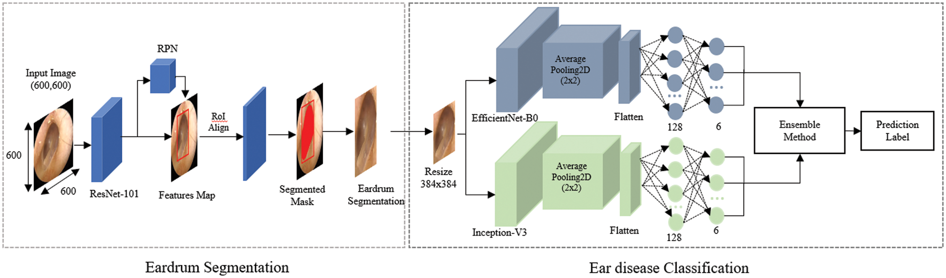
Figure 1: Overall architecture of the proposed approach

2.1 Dataset

The Soonchunhyang Cheonan Hospital provided 4,808 otoscopic images (normal: 2,040, TMPs: 356, AOM: 804, COM: 824, CC: 384, and OME: = 400), all of which were 600 pixels in both height and width, in joint photographic experts group (JPG) format. Of the 2,040 normal images, 410 were used for the eardrum region segmentation. The remaining 4,398 images were used for the multi-class classification network for normal, TMPs, AOM, COM, CC, and OME. The Institutional Review Board (IRB) of the hospital approved this retrospective investigation of medical records (IRB no. SCHCA 2020-02-022). Informed consent was waived. The relevant guidelines and regulations performed all methods. Fig. 2 shows the collected dataset’s otoscopic images with different labels of normal, TMPs, AOM, COM, CC, and OME.

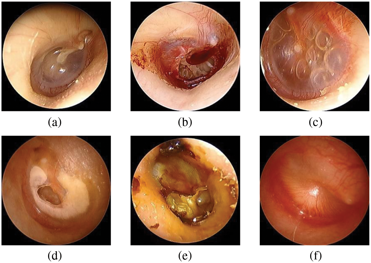
Figure 2: Examples of otoscopic images in the datasets. (a) Normal. (b) TMPs. (c) AOM. (d) COM. (e) CC. (f) OME

To evaluate the performance of our segmentation network, the gold-standard eardrum contours were obtained from all 410 ear images by two trained otolaryngologists. Initially, two trained otolaryngologists drew the contours, and confirmed them together.

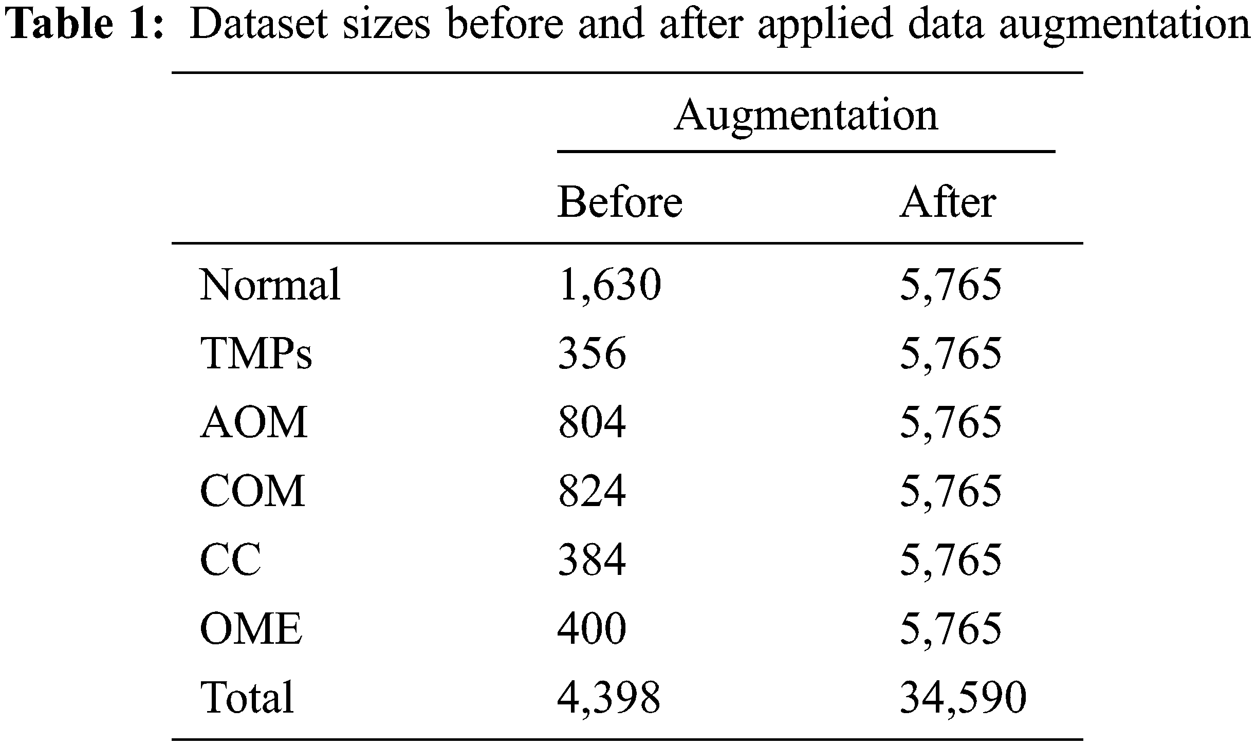
The enhanced 4,398 images are utilized in the multi-class classification network to balance the data for each class and avoid an overfitting problem [35]. Data augmentation is performed, including rotation, enlargement, vertical inversion, and brightness control. Therefore, after data augmentation processing, each class comprises 5,765 images, and total of 34,590 images. Table 1 summarizes the numbers of original data and augmented data for the multi-class classification.

2.2 Segmentation Network

Our segmentation network aims to extract eardrum contour from an otoscopic image. The segmentation network architecture is shown in Fig. 3. Two separate models, EfficientNetB0 [36] and Inception-V3 [37], are adopted with Mask R-CNN. The training objective is

argminθL(θ) (1)

where L(θ) is the binary cross-entropy loss, θ denotes the segmentation network parameter set composed of filter kernel weights and biases. Specifically, L(θ) is defined as

L(θ)=−1Nbatch⋅Npixel∑jNbatch⁡∑i=1Npixel⁡yi,jlog⁡(pθ(yi,j))+(1−yi,j)log⁡(1−pθ(yi,j)) (2)

where pθ(yi,j) denotes the softmax probability of the i-th pixel in the j-th otoscopic image, yi,j is the label (1 for the eardrum regions and 0 for background), Npixel is the number of pixels in one image, and Nbatch is batch size. The otoscopic images can be provided by different resources, which induce different image sizes, acquisition conditions, and scanning protocols. For the issue, we performed the preprocessing, which contrasted the limited adaptive histogram equalization (CLAHE) algorithm and resized the image size to 384 × 384 pixels.

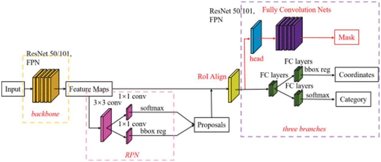
Figure 3: Segmentation network architecture

In this study, the segmentation network is Mask R-CNN trained on the COCO dataset [38]. Then the Mask R-CNN is pretrained with preprocessed data to combine the knowledge obtained from the previous training with the second task (eardrum segmentation). The EfficientNetB0 and Inception-V3 as backbones were selected for fine-tuning. Finally, we trained the models separately and evaluated the weights for the final ensemble model. Network parameters were initialized by Glorot initializer, which draws samples from a uniform distribution within 6fanin+fanout , where fanin and fanout are the number of input and output units, respectively [39].

2.3 Multi-Label Classification Network

The classification network aims to classify an otoscopic image into six categories: normal, TMPs, AOM, COM, CC, and OME. Similar to the segmentation network, two models of EfficientNetB0 and Inception-V3 are adopted and separately trained. The pre-processed images were first masked with the eardrum images from the segmentation networks, which were then fed into a classification network. The two separated CNN models of EffientNet-B0 and Inception-V3 were modified and added new fully connected layers, a GlobalAveragePooling2D layer, and two dense layers. The SoftMax activation function (at the output stage for the six classes) is used at the last of a dense layer with an output vector of six. The probability outputs for the six classes according to each model were combined by averaging; the predicted label is a class with a maximum output probability. Given the segmentation network parameter set α , the training loss function is

L(∝)=−1Nbatch∑iNbatch⁡∑c=16⁡yc,ilog⁡(p∝(yc,i)) (3)

where p∝(yc,i) denotes the softmax probability for the i-th image corresponding to the true label c (i.e., c∈{normal, TMPs, AOM, COM, CC and OME} ).

Pre-trained parameters from ImageNet were used for network weight initialization for network training. Subsequently, the network was trained using the otoscopic images. The model was trained using an Adadalta optimizer [40] with an initial learning rate of 0.0001 and adopted an early stopping strategy based on validation performance. The train stopped if the loss did not decrease by more than 0.001 over 20 epochs. A batch size of 16 was used. Weight decay and L2 regularization were applied to prevent overfitting problems. The classification network was also implemented by TensorFlow and the Keras libraries [41].

2.4 Application for Otitis diagnosis

The proposed approach is implemented as a web service using Flask [42] to provide easy access to detect ear diseases. Fig. 4 shows a web service for diagnosing ear diseases, including registration, login, upload, loading screens, and prediction results. After a user logged in to the web application and inputs otoscopic images, and then the predicted class is presented.

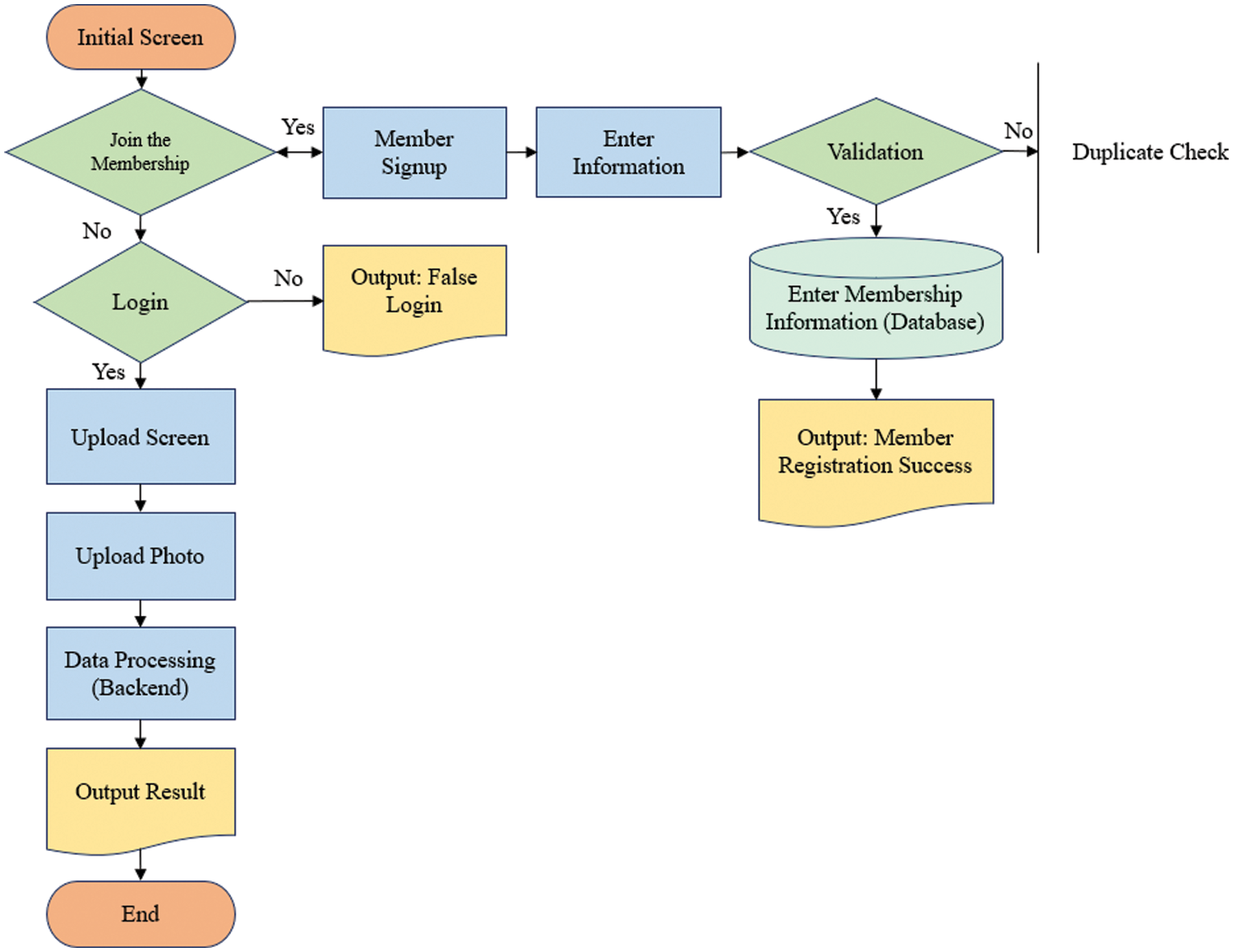
Figure 4: Flowchart of accessing to the web server for diagnosis of ear diseases

2.5 Evaluation Matric

The performance of the proposed method was evaluated using the disc similarity coefficient (DSC) for the segmentation and accuracy of the classification. For the segmentation, we first calculated the true positive (TP), false positive (FP), true negative (TN), and false negative (FN) values. TP (FP) is the number of positive pixels labelled correctly (incorrectly). TN (FN) is the number of negative pixels labelled correctly (incorrectly). Then, the DSC can be calculated as

DSC= 2TP2TP+FP+FN (4)

The DSC is the most commonly used metric for determining false positives and negative segmentation. It is a statistical approach used to compare the similarity of two data sets, which we used to determine the similarity between the estimated contour and the gold standard. The DSC value ranges between 0 and 1, where 0 means that there is no similarity and 1 means that there is perfect similarity.

For the classification, we also calculated the true positive (TP), false positive (FP), true negative (TN), and false negative (FN) values. Then, we obtained the accuracy as

Accuracy= TP+TNTP+TN+FP+FN×100 (%) (5)

In addition, along with accuracy, we presented the confusion matrix for the multi-classification performance evaluation.

3  Results

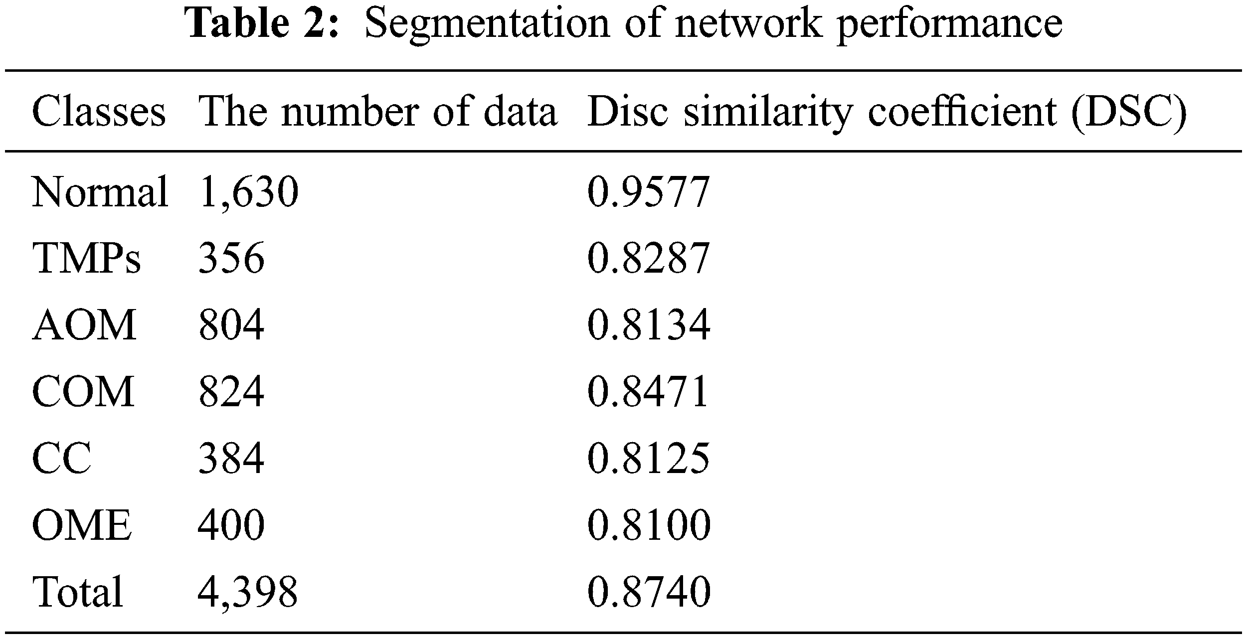
The eardrum region segmentation network was tested on 4,398 ear images, and the segmentation performance was accessed by calculating DSC. Table 2 summarizes the DSC of segmentation according to each label. For all classes, the DSC value is 0.8740. More specifically, the DSC value of the normal images is 0.9577. For TMPs, AOM, COM, CC and OME, the DSC values of 0.8277, 0.8134, 0.8471, 0.8125, and 0.8100, respectively. Since the segmentation network was trained using only normal images, it provided a higher DSC value for normal than for other labels.

For the classification performance evaluation, several models were trained, such as VGG19 [43], Resnet50 [44], Resnet101 [45], Resnet152 [46], Inception-V3, and EfficientNet-B0, and their performances were compared to our proposed classification model. The proposed classification model and the chosen CNN models were trained using the same hyper-parameters, the Adadelta activation function, the sparse categorical cross-entropy loss function, and the training rate of 0.1. To obtain training, validation, and test data, five-fold cross-validation (CV) was performed. Moreover, the early-stopping was used during model training to prevent overfitting [47]. Table 3 summarizes the performance comparison based on a five-fold CV. The results show that the accuracy of the proposed model is higher than the well-known CNN models along the five folds; the averaged accuracy of the five-fold cross-validation of the proposed method is 96.79%.

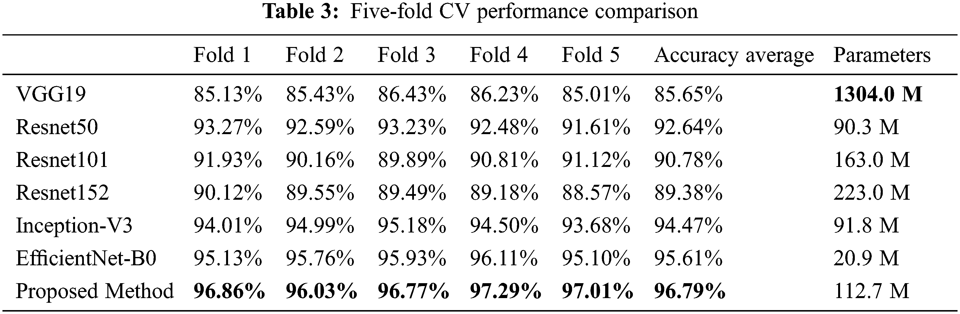
Fig. 5 shows the confusion matrix of the proposed method. Among 1,139 images of a normal class, 1,126 images were correctly classified, which corresponds to an accuracy of 98.86%. The other class of images were successfully identified as follows: 1,088 TMP images (95.52% accuracy), 1,082 AOM images (95.00% accuracy), 1,139 COM images (100% accuracy), 1,075 CC images (94.38% accuracy), and 1,139 OME images (100% accuracy).

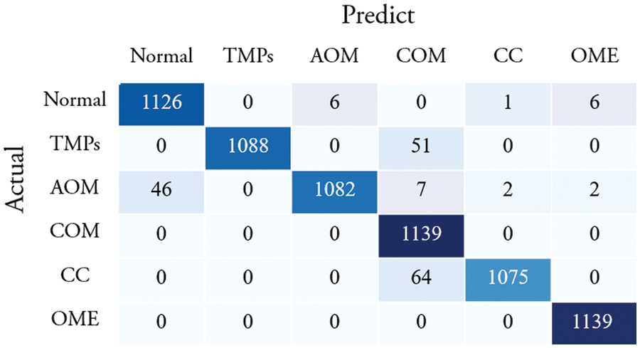
Figure 5: Confusion matrix of the proposed method

Fig. 6 compares the performance of using original eardrum images and preprocessed eardrum images for various models. In addition, the performance of the individual model with and without preprocessing was compared. The graph shows that the proposed classification model obtained higher accuracy than any other model for both kinds of images. For the same model, classification using preprocessed eardrum images obtained a higher performance than the classification without image processing. This show that the preprocessing with CLACHE increases the classification accuracy over all seven models.

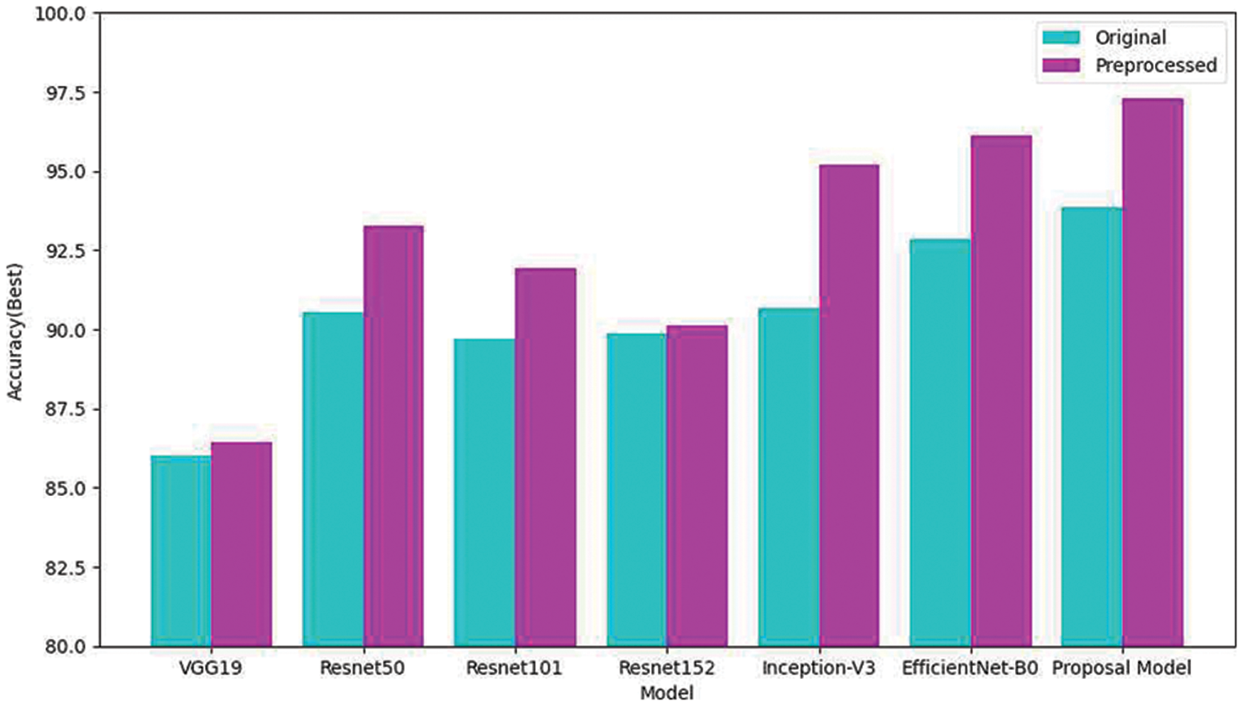
Figure 6: Comparison of classifications of the original and reconstructed datasets

Table 4 compares the proposed method for middle ear disease classification with other studies. In Table 4, Cha et al. [30] used ensemble deep TL with the Inception-V3 and RestNet101 models to detect six classes of eardrum images; an average accuracy of five-fold cross-validation was 93.67%. Camalan et al. [31] used TL to distinguish otoscopic images into three classes. The model was trained with 10-fold cross-validation and achieved a test accuracy of 80.58%. Sundgaard et al. [32] employed deep metric learning to detect three classes of ear disease and obtained an accuracy of 84.00%. In another study, Viscaino et al. [33] deployed three machine learning algorithms that extracted three features for distinguishing four classes. The result was that the support vector machine performed best with an average accuracy of 93.9%. In addition, Khan et al. [34] used a CNN model to automatically detect normal images and disease images named COM and OME from otoendoscopic images. The result achieved an accuracy of 95%. Previous studies focused on feature extraction and used single classifiers rather than defining ROIs and then applying an ensemble of classifiers. As the result, three- or four-class-split classifications afforded less than 96% accuracy, and one study distinguishing six classes had an accuracy of 93.67%.

The proposed model was trained and tested on a Windows 10 operating system with an Intel (R) Xeon (R) Silver 4114@2.20 GHz CPU, 192 GB of RAM, and an NVIDIA TITAN RTX 119 GB GPU. Fig. 7 shows deploying the proposed method to the web application. Fig. 7a shows the loading process of diagnosing ear diseases, and Fig. 7b shows the diagnosis results. Uploading the image requires about 0.8 s for an image with a resolution of 384 × 384 pixels; the smaller image, faster response speed. After a user input otoscopic images, the segmentation and classification networks segment and predict the type of ear diseases. When using the TensorFlow-GPU, about 8 s were required to allocate GPU resources, but this decreased to about 0.8 s using the CPU version.

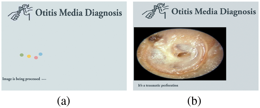
Figure 7: Ear disease diagnosis web service. (a) The loading screen (b) a result of the diagnosis

4  Discussion and Conclusion

In this study, we presented the segmentation and classification networks to detect the useful location in images and classify an otoscopic image into six categories: normal, TMPs, AOM, COM, CC, and OME. More specifically, the segmentation network based on Mask R-CNN is presented for extracting eardrums from images, and the classification network is based on an ensemble of Inception-V3 and EfficientNetB0. The proposed model provided higher CV accuracy of 97.29% than other the well-known CNN models and previous studies in the literature review. The achieved accuracy indicates that our method could be more applicable in a clinical decision-supporting system.

However, this study has several limitations. First, the proposed model was validated using a five-fold CV. It may be necessary to validate our model with external datasets such as prospectively collected data. To validate and update, we plan to deploy the proposed model on a public website so that anyone can classify the six labels using otoscopic images. Opening the AI model to the public helps validate and improve its performance. Second, our data did not include patients of other races, such as Caucasians or Middle East Asians. In the near future, we plan to apply our model to various datasets, including data from patients of other races.

Acknowledgement: Yunyoung Nam and Seong Jun Choi contributed equally to this work.

Funding Statement: This study was supported by a Basic Science Research Program through the National Research Foundation of Korea (NRF) funded by the Ministry of Science, ICT & Future Planning NRF-2020R1A2C1014829 and the Soonchunhyang University Research Fund.

Conflicts of Interest: The authors declare that they have no conflicts of interest to report regarding the present study.

References

    1. S. Y. Jung, D. Kim, D. C. Park, E. H. Lee, Y. -S. Choi et al., “Immunoglobulins and transcription factors in otitis media,” International Journal of Molecular Sciences, vol. 22, no. 6, pp. 3201, 2021. [Google Scholar]

    2. T. Otteson, “Otitis media and tympanostomy tubes,” Pediatric Clinics, vol. 69, no. 2, pp. 203–219, 2022. [Google Scholar]

    3. Y. G. Dabholkar, A. Wadhwa and A. Deshmukh, “A study of knowledge, attitude and practices about otitis media in parents in Navi-Mumbai,” Journal of Otology, vol. 16, no. 2, pp. 89–94, 2021. [Google Scholar]

    4. K. Kazahaya and W. P. Potsic, “Congenital cholesteatoma,” Current Opinion in Otolaryngology & Head and Neck Surgery, vol. 12, no. 5, pp. 398–403, 2004. [Google Scholar]

    5. Y. M. Wang, Y. Li, Y. S. Cheng, Z. Y. He, J. M. Yang et al., “Deep learning in automated region proposal and diagnosis of chronic otitis media based on computed tomography,” Ear Hear, vol. 41, no. 3, pp. 669–677, 2020. [Google Scholar]

    6. M. E. Jellinge, S. Kristensen and K. Larsen, “Spontaneous closure of traumatic tympanic membrane perforations: An observational study,” The Journal of Laryngology & Otology, vol. 129, no. 10, pp. 950–954, 2015. [Google Scholar]

    7. W. L. Niermeyer, R. H. W. Philips, G. F. Essig and A. C. Moberly, “Diagnostic accuracy and confidence for otoscopy: Are medical students receiving sufficient training?,” The Laryngoscope, vol. 129, no. 8, pp. 1891–1897, 2019. [Google Scholar]

    8. E. Demir, S. Topal, G. Atal, M. Erdil, Z. O. Coskun et al., “Otologic findings based on no complaints in a pediatric examination,” International Archives of Otorhinolaryngology, vol. 23, no. 1, pp. 36–40, 2019. [Google Scholar]

    9. P. Chang and K. Pedler, “Ear examination--a practical guide,” Australian Family Physician, vol. 34, no. 10, pp. 857–862, 2005. [Google Scholar]

  10. M. J. Donnelly, M. S. Quraishi and D. P. McShane, “ENT and general practice: A study of pediatric ENT problems seen in general practice and recommendations for general practitioner training in ENT in Ireland,” Irish Journal of Medical Science, vol. 164, no. 3, pp. 209–211, 1995. [Google Scholar]

  11. M. P. Paing, A. Sento, T. H. Bui and C. Pintavirooj, “Instance segmentation of multiple myeloma cells using deep-wise data augmentation and mask R-CNN,” Entropy, vol. 24, no. 1, pp. 134, 2022. [Google Scholar]

  12. Y. Lei, Z. Tian, S. Kahn, W. J. Curran, T. Liu et al., “Automatic detection of brain metastases using 3D Mask RCNN for stereotactic radiosurgery,” in Medical Imaging 2020: Computer-Aided Diagnosis. vol. 11314. Texas, USA: SPIE-International Society for Optics and Photonics, pp. 686–691, 2020. [Google Scholar]

  13. M. G. Crowson, J. Ranisau, A. Eskander, A. Barbier, B. Xu et al., “A contemporary review of machine learning in otolaryngology-head and neck surgery,” The Laryngoscope, vol. 130, no. 1, pp. 45–51, 2019. [Google Scholar]

  14. D. Bing, J. Ying, J. Miao, L. Lan, D. Wang et al., “Predicting the hearing outcome in a sudden sensorineural hearing loss via machine learning models,” Clinical Otolaryngology, vol. 43, no. 3, pp. 868–874, 2018. [Google Scholar]

  15. J. R. Dubno, M. A. Eckert, F. S. Lee, L. J. Matthews and R. A. Schmiedt, “Classifying human audiometric phenotypes of age-related hearing loss from animal models,” Journal of the Association for Research in Otolaryngology, vol. 14, no. 5, pp. 687–701, 2013. [Google Scholar]

  16. S. H. Fang, Y. Tsao, M. J. Hsiao, J. Y. Chen, Y. H. Lai et al., “Detection of pathological voice using cepstrum vectors: A deep learning approach,” Journal of Voice, vol. 33, no. 5, pp. 634–641, 2018. [Google Scholar]

  17. I. Mironică, C. Veteran and D. C. Gheorghe, “Automatic pediatric otitis detection by classification of global image features,” in Proc. 2011 E-Health and Bioengineering Conf. (EHB), Lasi, Romania, pp. 1–4, 2011. [Google Scholar]

  18. C. Veteran, D. C. Gheorghe and B. Ionescu, “Eardrum color content analysis in video-otoscopy images for the diagnosis support of pediatric otitis,” in Proc. ISSCS, 2011-Int. Symp. on Signals, Circuits and Systems, Lasi, Romania, pp. 1–4, 2011. [Google Scholar]

  19. Y. Huang and C. P. Huang, “A depth-first search algorithm based otoscope application for real-time otitis media image interpretation,” in 2017 18th Int. Conf. on Parallel and Distributed Computing, Applications and Technologies (PDCAT), Taipei, Taiwan, pp. 170–175, 2017. [Google Scholar]

  20. H. C. Myburgh, S. Jose, D. W. Swanepoel and C. Laurent, “Towards low cost automated smartphone-and cloud-based otitis media diagnosis,” Biomedical Signal Processing and Control, vol. 39, no. 6, pp. 34–52, 2018. [Google Scholar]

  21. C. Zafer, “Fusing fine-tuned deep features for recognizing different tympanic membranes,” Biocybernetics and Biomedical Engineering, vol. 40, no. 1, pp. 40–51, 2020. [Google Scholar]

  22. J. Y. Lee, S. H. Choi and J. W. Chung, “Automated classification of the tympanic membrane using a convolutional neural network,” Applied Sciences, vol. 9, no. 9, pp. 1827, 2019. [Google Scholar]

  23. L. Cai, T. Long, Y. Dai and Y. Huang, “Mask R-CNN-based detection and segmentation for pulmonary nodule 3D visualization diagnosis,” IEEE Access, vol. 8, pp. 44400–44409, 2020. [Google Scholar]

  24. B. Xu, W. Wang, G. Falzon, P. Kwan, L. Guo et al., “Automated cattle counting using mask R-CNN in the quadcopter vision system,” Computers and Electronics in Agriculture, vol. 171, no. 1, pp. 105300, 2020. [Google Scholar]

  25. K. He, G. Gkioxari, P. Dollár and R. Girshick, “Mask R-CNN,” in Proc. IEEE Int. Conf. on Computer Vision, Venice, Italy, pp. 2961–2969, 2017. [Google Scholar]

  26. J. H. Shu, F. D. Nian, M. H. Yu and X. Li, “An improved mask R-CNN model for multiorgan segmentation,” Mathematical Problems in Engineering, vol. 2020, pp. 1–11, 2020. [Google Scholar]

  27. T. Shibata, A. Teramoto, H. Yamada, N. Ohmiya and K. Saito, “Automated detection and segmentation of early gastric cancer from endoscopic images using mask R-CNN,” Applied Sciences, vol. 10, no. 11, pp. 3842, 2020. [Google Scholar]

  28. S. Khan, N. Islam, Z. Jan, I. U. Din and J. J. P. C. Rodrigues, “A novel deep learning-based framework for the detection and classification of breast cancer using transfer learning,” Pattern Recognition Letters, vol. 125, no. 6, pp. 1–6, 2019. [Google Scholar]

  29. S. Niu, M. Liu, Y. Liu, J. Wang and H. Song, “Distant domain transfer learning for medical imaging,” IEEE Journal of Biomedical and Health Informatics, vol. 25, no. 10, pp. 3784–3793, 2021. [Google Scholar]

  30. D. Cha, C. Pae, S. B. Seong, J. Y. Choi and H. J. Park, “Automated diagnosis of ear disease using deep ensemble learning with a big otoendoscopy image database,” EbioMedicine, vol. 45, pp. 606–614, 2019. [Google Scholar]

  31. S. Camalan, M. K. Niazi, A. C. Moberly, T. Teknos and G. Essig, “OtoMatch: Content-based eardrum image retrieval using deep learning,” PLoS One, vol. 15, no. 5, pp. e0232776, 2020. [Google Scholar]

  32. J. V. Sundgaard, J. Harte, P. Bray, S. Laugesen and Y. Kamide, “Deep metric learning for otitis media classification,” Medical Image Analysis, vol. 71, no. March, pp. 102034, 2021. [Google Scholar]

  33. M. Viscaino, J. C. Maass, P. H. Delano, M. Torrente and C. Stott, “Computer-aided diagnosis of external and middle ear conditions: A machine learning approach,” PLoS One, vol. 15, no. 3, pp. e0229226, 2020. [Google Scholar]

  34. M. A. Khan, S. Kwon, J. Choo, S. M. Hong, S. H. Kang et al., “Automatic detection of the tympanic membrane and middle ear infection from oto-endoscopic images via convolutional neural networks,” Neural Networks, vol. 126, no. 115, pp. 384–394, 2020. [Google Scholar]

  35. J. Cui, X. Zhang, F. Xiong and C. -L. Chen, “Pathological myopia image recognition strategy based on data augmentation and model fusion,” Journal of Healthcare Engineering, vol. 2021, no. 7, pp. 1–15, 2021. [Google Scholar]

  36. B. Rigaud, O. O. Weaver, J. B. Dennison, M. Awais, B. M. Anderson et al., “Deep learning models for automated assessment of breast density using multiple mammographic image types,” Cancers, vol. 14, no. 20, pp. 5003, 2022. [Google Scholar]

  37. C. Wang, D. Chen, L. Hao, X. Liu and Y. Zeng, “Pulmonary image classification based on inception-v3 transfer learning model,” IEEE Access, vol. 7, pp. 146533–146541, 2019. [Google Scholar]

  38. J. Meng, L. Xue, Y. Chang, J. Zhang and S. Chang, “Automatic detection and segmentation of adenomatous colorectal polyps during colonoscopy using mask R-CNN,” Open Life Sciences, vol. 15, no. 1, pp. 588–596, 2020. [Google Scholar]

  39. X. Glorot and Y. Bengio, “Understanding the difficulty of training deep feedforward neural networks,” in Proc. of the Thirteenth Int. Conf. on Artificial Intelligence and Statistics, Sardinia, Italy, PMLR, vol. 9, pp. 249–256, 2010. [Google Scholar]

  40. N. M. Halgamuge, E. Daminda and A. Nirmalathas, “Best optimizer selection for predicting bushfire occurrences using deep learning,” Natural Hazards, vol. 103, no. 1, pp. 845–860, 2020. [Google Scholar]

  41. J. Brownlee, “Develop your first neural network with keras” in Deep Learning with Python: Develop Deep Learning Models on Theano and TensorFlow Using Keras, 19th ed., vol. 1. Melbourne, Australia: Machine Learning Mastery, pp. 43–49, 2016. [Google Scholar]

  42. D. F. Ningtyas and N. Setiyawat, “Implementasi flask framework pada pembangunan aplikasi purchasing approval request,” Jurnal Janitra Informatika Dan Sistem Informasi, vol. 1, no. 1, pp. 19–34, 2021. [Google Scholar]

  43. A. Lumini and L. Nanni, “Deep learning and transfer learning features for plankton classification,” Ecological Informatics, vol. 51, pp. 33–43, 2019. [Google Scholar]

  44. S. T. Krishna and H. K. Kalluri, “Deep learning and transfer learning approaches for image classification,” International Journal of Recent Technology and Engineering (IJRTE), vol. 7, no. 5S4, pp. 427–432, 2019. [Google Scholar]

  45. S. Anjum, L. Hussain, M. Ali, M. H. Alkinani, W. Aziz et al., “Detecting brain tumours using deep learning convolutional neural network with a transfer learning approach,” International Journal of Imaging Systems and Technology, vol. 32, no. 1, pp. 307–323, 2021. [Google Scholar]

  46. Q. Guo, X. Yu and G. Ruan, “LPI radar waveform recognition based on deep convolutional neural network transfer learning,” Symmetry, vol. 11, no. 4, pp. 540, 2019. [Google Scholar]

  47. X. Ying, “An overview of overfitting and its solutions,” An Overview of Overfitting and Its Solutions, vol. 1168, no. 2, pp. 022022, 2019. [Google Scholar]