Hyperspectral Remote Sensing Image Classification Using Improved Metaheuristic with Deep Learning

1  Introduction

Remote sensing images (RSI) comprise a large number of applications. Remote images or data were captured by gadgets and designed for advanced learning. Hence, we can understand different aspects of the relevant areas [1]. Remote sensing scene classification (RSSC) could offer a sequence of semantic classes that could help classify land use and land cover. RSIs with higher spatial resolutions were the conventional category for RCCS. Therefore, RS is frequently used in target detection, urban mapping, natural resource management, and precision agriculture [2]. Lately, extensive attempts are being made to develop feature representation and classifiers for the task of RSI scene classifier in a wide range of applications [3]. Urban areas have been focused in recent times on remote sensing applications. Urban water and gas pollution, urban land cover classifications, urban flood, hard target detection, urban green space detection, and many more have arisen with the development and occurrence of RS imaging [4]. The RSI datasets show colour and texture information due to their higher spatial resolution. RSIs have many more scene classes and changes than conventional RSI and become highly difficult to identify with conventional pixel-related approaches [5]. Deep learning (DL) allows the object-level classification and recognition of RSI and a better understanding of the RSIs contents at the semantic levels.

In a period of huge data, DL exhibits interesting viewpoints. It undergoes unprecedented achievement in several applications [6]. DL utilizes machine learning (ML) approaches, including unsupervised or supervised strategies for learning hierarchical representation in deep networks. DL employs deep structures to deal with complicated relations between the class label and the input data [7]. DL and ensemble-related methods have been highly effective for multi-temporal and multisource RSI classifiers. DL has shown superior performance in feature extraction in multispectral and hyperspectral images like extraction of semantic segmentation, types of labels, recognition of objects and classes, and pixel-based classification [8]. DL methods study features in the data; lower-level features were derived from the spectral and texture and regarded as the bottom level. The topmost level becomes the representation of resultant features [9]. Indeed, several methods have expressed that the efficiency of the land cover scene classifier has significantly enhanced because of the robust features to robust feature representations learned by diverse DL structures [10].

This study introduces an Improved Slime Mould Optimization with a graph convolutional network for the hyperspectral remote sensing image classification (ISMOGCN-HRSC) model. In the presented ISMOGCN-HRSC model, the synergic deep learning (SDL) model is exploited to produce feature vectors. The GCN model is utilized for image classification purposes, enabling the identification of the proper class labels of the RSIs. The ISMO approach was used to enhance the classification efficiency of the GCN model, which is derived by integrating chaotic concepts into the SMO algorithm. The experimental assessment of the ISMOGCN-HRSC approach was tested using a benchmark dataset. The comparison study reported that the ISMOGCN-HRSC model shows promising performance over other DL models in the literature. In short, the paper's contribution is summarized as follows.

•   Develop an effective ISMOGCN-HRSC technique to classify hyperspectral remote sensing images.

•   Perform feature extraction using the SDL model for hyperspectral remote sensing image classification.

•   Propose an ISMO with a GCN model for the hyperspectral remote sensing image classification process.

•   Validate the results of the ISMOGCN-HRSC technique on IPI and PAU datasets.

The rest of the paper is organized as follows. Section 2 offers the related works, and Section 3 introduces the proposed model. Later, Section 4 provides performance validation, and Section 5 concludes the work.

2  Related Works

The authors in [11] modelled to utilize the 3D structure for extracting spectral-spatial data for framing a deep neural network (DNN) for Hyperspectral RSI (HIS) classification. Depending on DenseNet, the 3D closely connected convolutional network has been enhanced for learning spectral-spatial features of HSIs. The closely connected framework could improve feature communication, supports feature reusage, enhance data flow from the network, and induce deep network simpler for training data. The 3D-DenseNet contains a deep structure compared to 3D-CNN; therefore, it could study very powerful spectral-spatial features from HSIs. In [12], the authors devise an RS scene-classifier technique related to vision transformer. Such networks that were now identified as existing methods from natural language processing (NLP) do not depend on the convolution layer as in conventional neural networks (CNNs). Alternatively, it uses multi-head attention systems as the chief generating block for deriving long-range contextual relationships among pixels from the image. During the initial step, images in the study were classified into patches after being transformed into series by embedding and flattening.

In [13], the authors offer baseline solutions to declared complexity by advancing a general multi-modal DL (MDL) structure. Specifically, they also examine an unusual case of multimodality learning (MML)-cross-modality learning (CML), which occurs extensively in RSI classifier applications. The authors in [14] devise a deep CNN method which could categorize RS test data from a dataset distinct from the trained data. To achieve this, they initially retrained a ResNet-50 method employing EuroSAT, a large-scale RS data set for advancing a base method. Afterwards, they compiled Ensemble learning and Augmentation to enhance its generalizing capability. The authors in [15] formulate a novel RSSC-based error-tolerant deep learning (RSSC-ETDL) technique for mitigating the negative influence of incorrect labels on the RSI scene data set. In this devised RSSC-ETDL approach, learning multi-view CNNs and rectifying error labels was otherwise directed iteratively. To cause the alternative method to work efficiently, they frame a new adaptive multi-feature collaborative representation classifier (AMF-CRC), which helps adaptively integrate many features of CNNs to rectify the label of indefinite samples. The authors in [16] formulate an extensive and deep Fourier network for learning features proficiently through pruned features derived in the frequency domains. The derived feature was pruned to recall significant features and diminish computation.

The authors in [17] present a new deep convolutional CapsNet (DC-CapsNet) dependent upon spectral-spatial features for improving the efficiency of CapsNet from the HSI classifier but significantly decreasing the computation cost of this method. In detail, a convolution capsule layer dependent upon the growth of dynamic routing utilizing 3D convolutional was utilized to reduce the count of parameters and improve the robustness of learned spectral and spatial features. The authors in [18] examine a great HSI denoising approach named non-local 3DCNN (NL-3DCNN), which integrates typical ML and DL approaches. NL-3DCNN utilizes the higher spectral correlation of HSI utilizing subspace representation, and equivalent representation coefficients can be named eigenimages. The higher spatial correlation in Eigen images can be utilized by grouping non-local same patches that can be denoised by 3DCNN.

The authors in [19] propose a DL-based extracting feature process for a hyperspectral data classifier. Initially, the authors exploited an SDAE for extraction of the in-depth feature of HIS data: a huge count of unlabeled data can be pretrained for extracting the depth pixel features. The authors added arbitrary noise to the input layer of networks for generating a de-noising AE machine and further process inputs for recreating novel data. During the top layer, DNN has been fine-tuned by the Softmax regression classifier. The authors in [20] examine a full CNN for the HSI classifier. The knowledge of the present approach is that 2-D convolution layers learned the feature maps dependent upon the spectral-spatial data of HSI data, and the FC layers of CNN carried out the HSI classifier.

3  The Proposed Model

This study has recognised a novel ISMOGCN-HRSC approach for identifying and classifying RSIs. The SDL model is exploited in the presented ISMOGCN-HRSC approach to produce feature vectors. For image classification purposes, the ISMO with GCN model is utilized. Fig. 1 illustrates the overall process of the ISMOGCN-HRSC algorithm. As shown in the figure, the proposed model follows a series of operations namely image preprocessing, SDL-based feature extraction, GCN-based RSI classification, and SMO-based hyperparameter optimization.

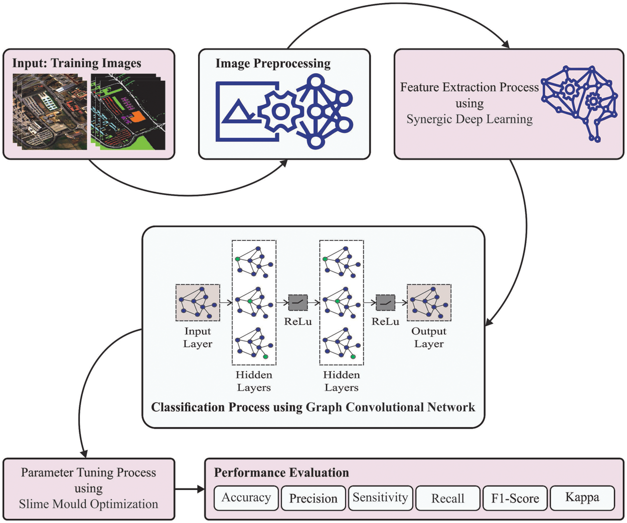
Figure 1: Overall process of ISMOGCN-HRSC approach for RSI classification

3.1 Synergic Deep Learning-Based Feature Extraction

In this work, the SDL model is exploited to produce feature vectors. Extracting feature is a procedure of dimensionality decrease by that the primary set of raw data has decreased for other controllable groups to process. A feature of these huge databases is a massive count of variables which need a lot of computing resources for processing. Extracting feature is the name for approaches that choose and integrate variables as to features, efficiently decreasing the count of managed data but still correctly and entirely describing the novel database. The procedure of extracting features is helpful if it is required to reduce the count of resources required to process without losing significant or relevant data. Extracting features also decreases the count of redundant data to provide a study. Similarly, the data reduction and the machine efforts in structure variable combination (feature) enable the DL procedure’s learning speed and generalized stages.

The presented SDL method refers to SDLn , comprises three main components: an image pair input layer n DCNN component and a Cn2 synergic network [21]. The input of the SDL method is a collection of arbitrarily chosen images rather than individual images. Every DCNN model of network architecture assists in learning representation independently from an image from the supervision of the true label of the input image. Then, we explore every three elements of the SDL method.

Pair Input Layer

Unlike conventional DCNN, the suggested SDLn mechanism concurrently accepts n input images that are arbitrarily chosen in the training set. Every image and its class labels are inputted into the DCNN module, and every pair of images has respective synergic labels that use a synergic network. For unifying the image size, we have resized all the images to 224×224×3 using the bi-cubic interpolation.

DCNN Component

As a result of the stronger representative ability of the prominent residual network, we employed a pre-trained fifty-layer RNN (ResNet50) as the initialisation of every DCNN component represented as DCNN i (i= 1,2, …, n) . Every DCNN module is trained by an image sequence X={x(1), x(2), …, x(M)} and a respective class label sequences Y={y(1),y(2), …,y(M)}, aims at finding a parameter set θ that minimalizes the subsequent cross-entropy loss

1(θ)=−1M[∑i=1M⁡∑j=1K⁡1{y(i)=j}log ezj(i)∑l=1k⁡ez1(i)]                      (1)

In Eq. (1), K refers to the class number, Z(i)=ℱ(x(i), θ) denotes forward computing. This optimization issue is resolved by using the mini-batch SGD approach. The attained set of parameters for DCNN i is represented as θ(i) , and the parameter is not shared amongst distinct DCNN modules.

Synergic Network

To supervise the training of every DCNN module through the synergic labels of every pair of images, we designed a synergic network comprising an embedded layer, an FC learning, and a resultant layer. Consider a pair of images (xA, xB) to be input into 2 DCNN modules (DCNN-i, DCNN-j), correspondingly. The resultant of the final FC layer from the DCNN is determined by the deep image feature learned by DCNN that is attained by ward computing, represented in the following

fA=ℱ(xA, θ(i))                    (2)

fB=ℱ(xB, θ(j))

Next, the deep feature of an image is concatenated by fA∘B and input as to synergic networks. The anticipated outcome is the synergic labels of an image pair that can be expressed by

yS(xA, xB)={1if yA=yB0if yA≠yB                         (3)

It can be advantageous to monitor the synergic signals by utilizing the subsequent binary cross-entropy loss and including additional sigmoid layers

1S(θs)=yS log yS^+(1−yS)log (1−yS^) (4)

In Eq. (4), the variable of the synergic network is represented as θS , and the forward computing of the synergic network is indicated as yS^= ℱ(fA∘B, θS) . Fig. 2 portrays the procedure of the SDL technique.

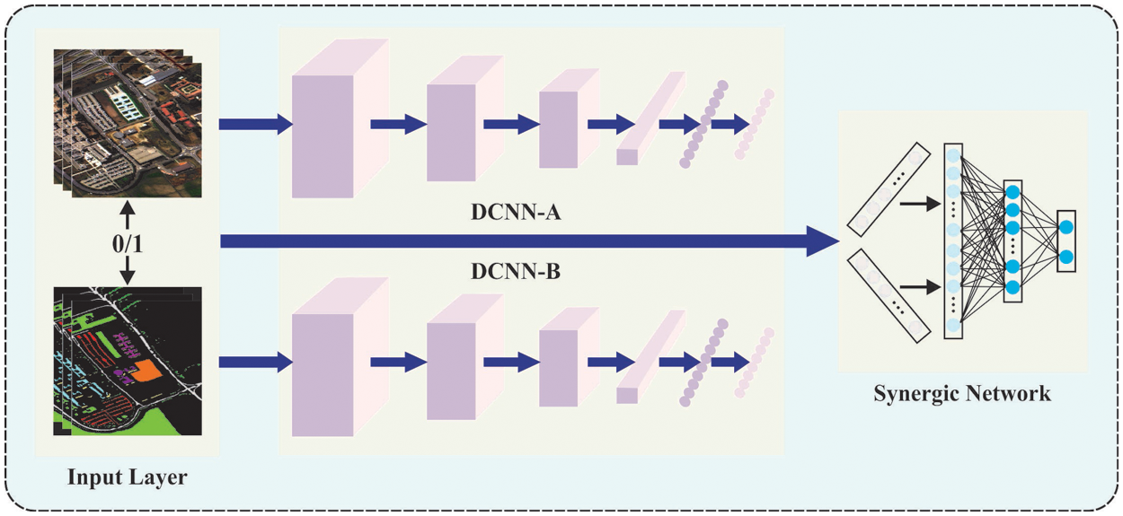
Figure 2: Procedure of SDL

3.2 Image Classification Using GCN Model

For image classification purposes, the GCN model is utilized. Intend to learn the relation-aware feature depiction of nodes through the propagation of the intrinsic data of graph structure. In contrast to the CNN-based method that operates convolution on local Euclidean structure, GCN generalizes the convolution function to non-Euclidean information (for example, graph) [22]. Especially accomplishes spectral GCN on the feature of neighbouring nodes and upgrades the feature representations of every node integrating the intrinsic structure data of the graph in the learning method.

Assumed a graph G=(V, E) with N node vi∈V(i=1, N) , edges (vi, vj)∈E and a neighbourhood matrix  A∈RN×N that defines the correlation of N nodes, GCN aims to encode the graph G through a NN mechanism f=(X, A) whereby X∈RlVκD denotes the original feature of N nodes. A multilayer GCN upgrades the node feature based on the subsequent layer-by-layer propagating rules:

H(l+1)=σ(D~−1/2A~D~−1/2H(l)W(l)) (5)

In Eq. (5), A~=A+IN denotes the neighbourhood matrix A with self-connection, IN refers to the identity matrix, and D~ii=∑j ⁡Aij~ indicates the degree matrix. W(l)∈Rdl×dl+1 shows a trained weight matrix, and σ denotes an activation function (ReLU). H(l)∈RN×dl represents the feature representation of the node; dl indicates the feature dimension, and H(l+1)∈RN×dl+1 shows the upgrade node feature. It should be noted that H(0)=X . Subsequently, the relation-aware feature representation of the node is attained by the message-passing model of the multilayer GCN.

3.3 Parameter Tuning Using ISMO Algorithm

The ISMO algorithm is used to improve the classification efficiency of the GCN approach, which is derived by integrating chaotic concepts into the SMO algorithm. SMO algorithm is a novel optimizer inspired by the natural SM oscillation mode. SMO algorithm exploits weight as the positive and negative feedback produced by mimicking the foraging method of SM, where oscillating, approaching food, and wrapping food are the three dissimilar forms [23]:

Approach Food

SM relies on the smell of the air to get closer to the desired food, and it is expressed as:

x(t+1)={xb(t)+vb×(W×xA(t)−xB(t))        r<p vc×x(t)                                            r≥p (6)

In Eq. (6), W denotes the weight of SMs. X(t) indicates the optimum global location, and x(t) represents the location of every SM. vb oscillates among [−a, a]. X(t) and X(t) are arbitrary locations. The formula of vc and W are given in Eqs. (8)–(10).

Here p is represented in the following:

p= tanh |Fit(i)−BF| (7)

In Eq. (7), Fit(i) denotes the fitness of every SM; BF indicates the optimal fitness of SM in the existing iteration.

vb=[a, a],a=arctanh (−t max iter) (8)

vc=[−b, b], b=1−t max iter    (9)

Amongst them, t specifies the existing iteration amount, and maxiter denotes the maximal iteration.

W is formulated below:

W (SmellIndex (i))={{1+r×log(BF−Fit(i)BF−WF+1)}condition{1−r×log(BF−Fit(i)BF−WF+1)}others (10)

SmellIndex=sort(Fit) (11)

SmellIndex is the series of fitness values afterwards arranged. r denotes an arbitrary value within zero and one; the condition specifies that Fit(i) is ordered in the first half.

WRAP FOOD

This section exploits a mathematical expression for stimulating the shrinkage of SM. The negative and positive feedback amongst food concentrations is formulated in Eq. (5). Once the food concentration of the region is higher, the weight close is larger, and once the food concentration nearer the region is lower, the weight near reductions to discover other regions as:

x(t+1)={rand×(UB−LB)+LB                      rand<zxb(t)+vb×(W×xA(t)−xB(t))         r<pvc×x(t)                                            r≥p (12)

Whereas UB and LB embody the upper and lower limits of the overall space. z is frequently considered as a small value, 0.03. The definition of vb, VC, W, p, xb,xA , and xB are given in Eq. (6).

OSCILLATION

The SM, for a major part, changes the cytoplasm flow in the vein through the propagative wave produced using the biological vibrator to be located in the best food concentration location. To mimic the variations in the pulse width of SM bacteria, vb , and VC are employed to accomplish these variations.

The mathematical method is applied to stimulate the vibrational frequency of food concentration. vb is produced arbitrarily within [−a, a] and approaches 0 with the maximum iteration count. VC is within the interval [−1, 1] and lastly obtains zero.

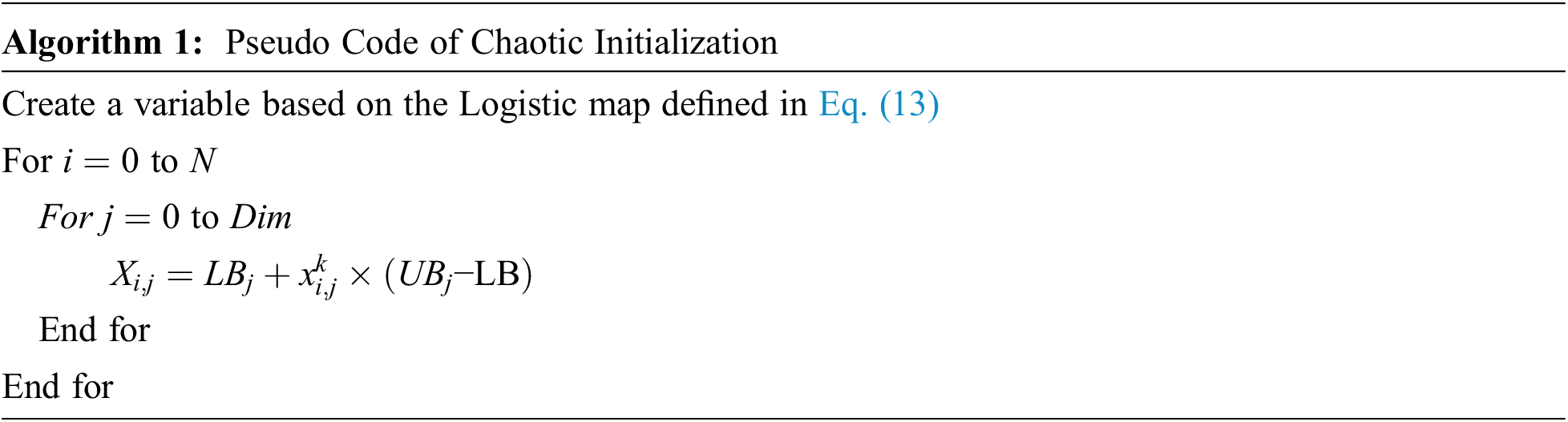
In this study, the ISMO algorithm is derived by integrating chaotic concepts into the SMO algorithm. Amongst the existing chaotic searching approaches, logistic chaotic mapping is commonly utilized. Because of easier functioning and optimal performance, the ISMO algorithm makes use of the chaotic map for population initialization to accomplish acceleration in the earlier process. The logistic map can be determined as follows

xk+1=a×xk(1−xk) (13)

where a denotes the real number (a=4), k represents the present round, and xk denotes the kth chaotic number.

The ISMO system grows a fitness function (FF) for accomplishing higher classifier performance. It solves a positive integer for representing an optimum performance of candidate outcomes. During this analysis, the minimizing of classifier error rate has supposed that FF, as determined in Eq. (14).

fitness(xi)=Classifier Error Rate(xi)=number of misclassified samples total number of samples∗100                   (14)

4  Experimental Validation

The experimental validation of the ISMOGCN-HRSC approach is tested utilizing 2 datasets, namely Indian Pines (IPI) dataset [24] and Pavia University (PAU) dataset [25]. The IPI dataset is a Hyperspectral image segmentation dataset. The input data consists of hyperspectral bands over a single landscape in Indiana, US (Indian Pines data set) with 145 × 145 pixels. For each pixel, the data set contains 220 spectral reflectance bands. The PAU dataset is a hyperspectral image dataset collected by a sensor known as the reflective optics system imaging spectrometer (ROSIS-3) over the city of Pavia, Italy. It has 610 × 340 pixels with 115 spectral bands. The image is separated into 9 classes with a total of 42,776 labelled samples, comprising asphalt, meadows, gravel, trees, metal sheet, bare soil, bitumen, brick, and shadow.

Fig. 3 shows the confusion matrices created by the ISMOGCN-HRSC method on the classification of RS images under the IPI dataset. The figures reported that the ISMOGCN-HRSC model has proficiently categorized all 16 class labels.

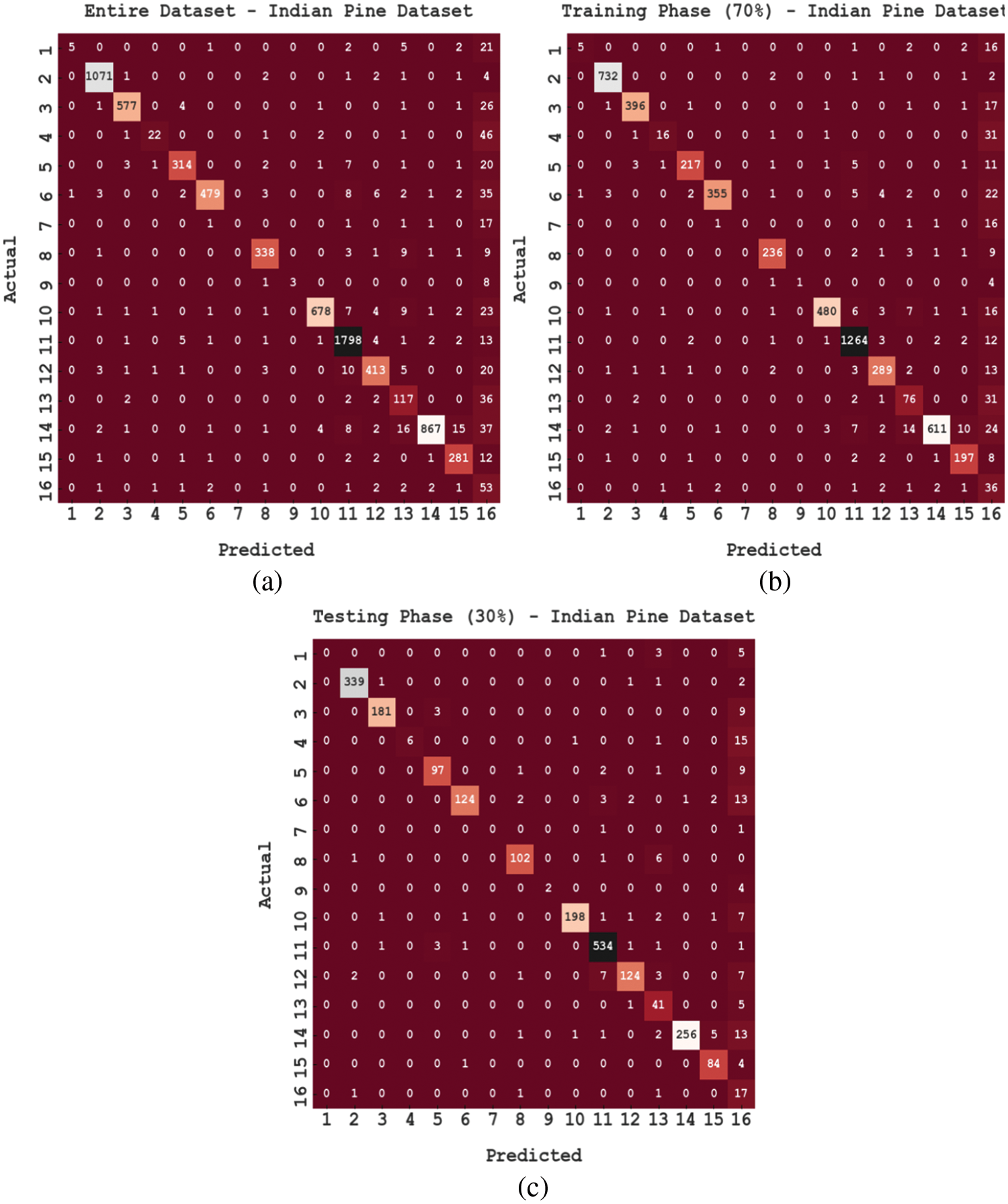
Figure 3: Confusion matrices of ISMOGCN-HRSC approach under IPI dataset (a) Entire dataset, (b) 70% of TR data, and (c) 30% of TS data

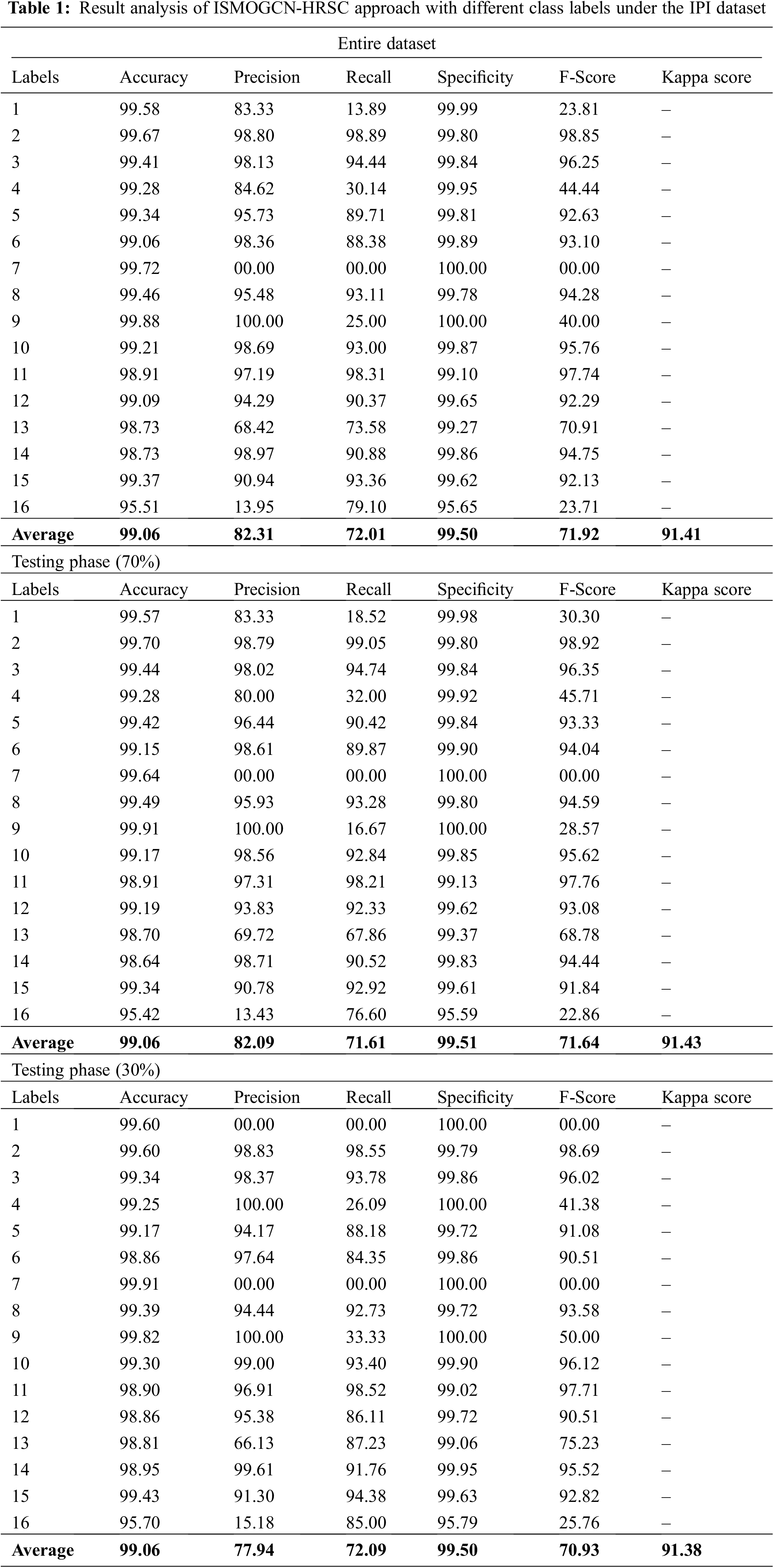
Table 1 provides an overall RS image classification outcome of the ISMOGCN-HRSC model on the IPI dataset. The obtained values demonstrated that the ISMOGCN-HRSC model had shown enhanced performance under each class. For instance, on the entire dataset, the ISMOGCN-HRSC model has gained average accuy , precn , recal , specy , Fscore , and kappa of 99.06%, 82.31%, 72.01%, 99.50%, 71.92%, and 91.41% respectively. Meanwhile, on 70% of training (TR) data, the ISMOGCN-HRSC approach has reached average accuy , precn , recal , specy , Fscore , and kappa of 99.06%, 82.09%, 71.61%, 99.51%, 71.64%, and 91.43% correspondingly. Eventually, on 30% of testing (TS) data, the ISMOGCN-HRSC system has reached average accuy , precn , recal , specy , Fscore , and kappa of 99.06%, 77.94%, 72.09%, 99.50%, 70.93%, and 91.38% correspondingly.

The training accuracy (TRA) and validation accuracy (VLA) acquired by the ISMOGCN-HRSC system on the IPI dataset is showcased in Fig. 4. The experimental result exposed that the ISMOGCN-HRSC approach has been able to improve values of TRA and VLA. Mostly the VLA looked that superior to TRA.

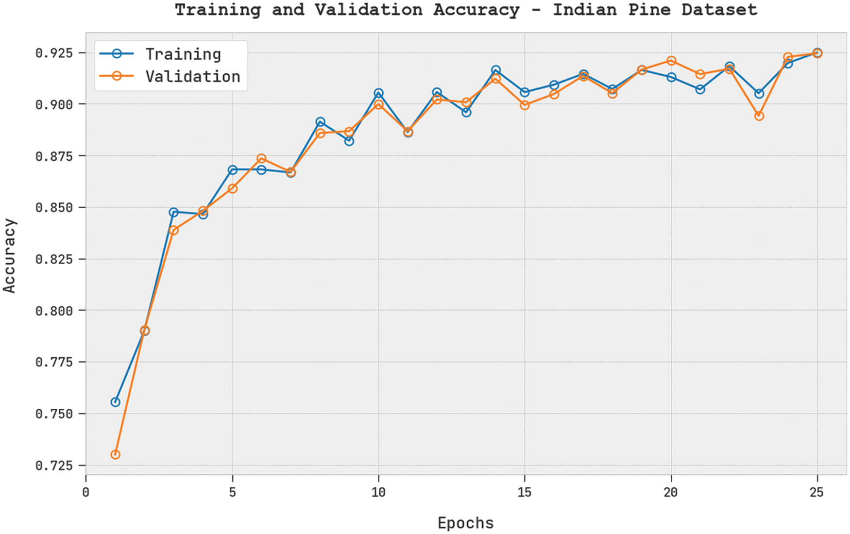
Figure 4: TRA and VLA analysis of ISMOGCN-HRSC approach under the IPI dataset

Table 2 offers an overall RS image classification outcome of the ISMOGCN-HRSC approach on the PAU dataset. The obtained values show that the ISMOGCN-HRSC methodology has enhanced performance under each class. For the sample, on the entire dataset, the ISMOGCN-HRSC technique has attained average accuy , precn , recal , specy , Fscore , and kappa of 98.93%, 91.24%, 91.09%, 99.37%, 91.10%, and 93.62% correspondingly. In the meantime, on 70% of TR data, the ISMOGCN-HRSC approach has reached average accuy , precn , recal , specy , Fscore , and kappa of 98.93%, 91.20%, 91.09%, 99.37%, 91.08%, and 93.64% respectively. Finally, on 30% of TS data, the ISMOGCN-HRSC methodology has gained average accuy , precn , recal , specy , Fscore , and kappa of 98.92%, 91.32%, 91.09%, 99.36%, 91.15%, and 93.57% correspondingly.

Table 3 indicates the comparative results of the ISMOGCN-HRSC model with other existing models on the IPI dataset. The results inferred that the ISMOGCN-HRSC model had shown enhanced results over other models. For instance, concerning accuy , the ISMOGCN-HRSC model has attained an improved accuy of 99.06%, whereas the SVMT, SVMEPFT, CoSVMT, CoSVM-EPFT, GFSVMT, and GFSVMEPFT models have obtained reduced accuy of 81.06%, 89.65%, 90.78%, 90.98%. 94.91% and 95.37%, respectively. Also, concerning kappa , the ISMOGCN-HRSC approach has achieved an enhanced kappa of 91.38%, whereas the SVMT, SVMEPFT, CoSVMT, CoSVM-EPFT, GFSVMT, and GFSVMEPFT algorithms have acquired minimal kappa of 69.18%, 66.77%, 68.91%, 71.40%. 74.22%, and 75.40% correspondingly.

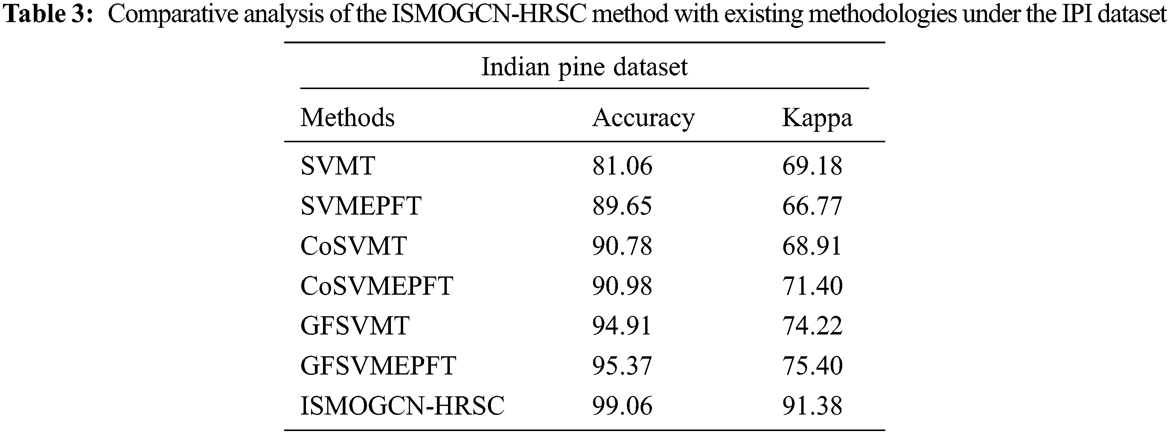
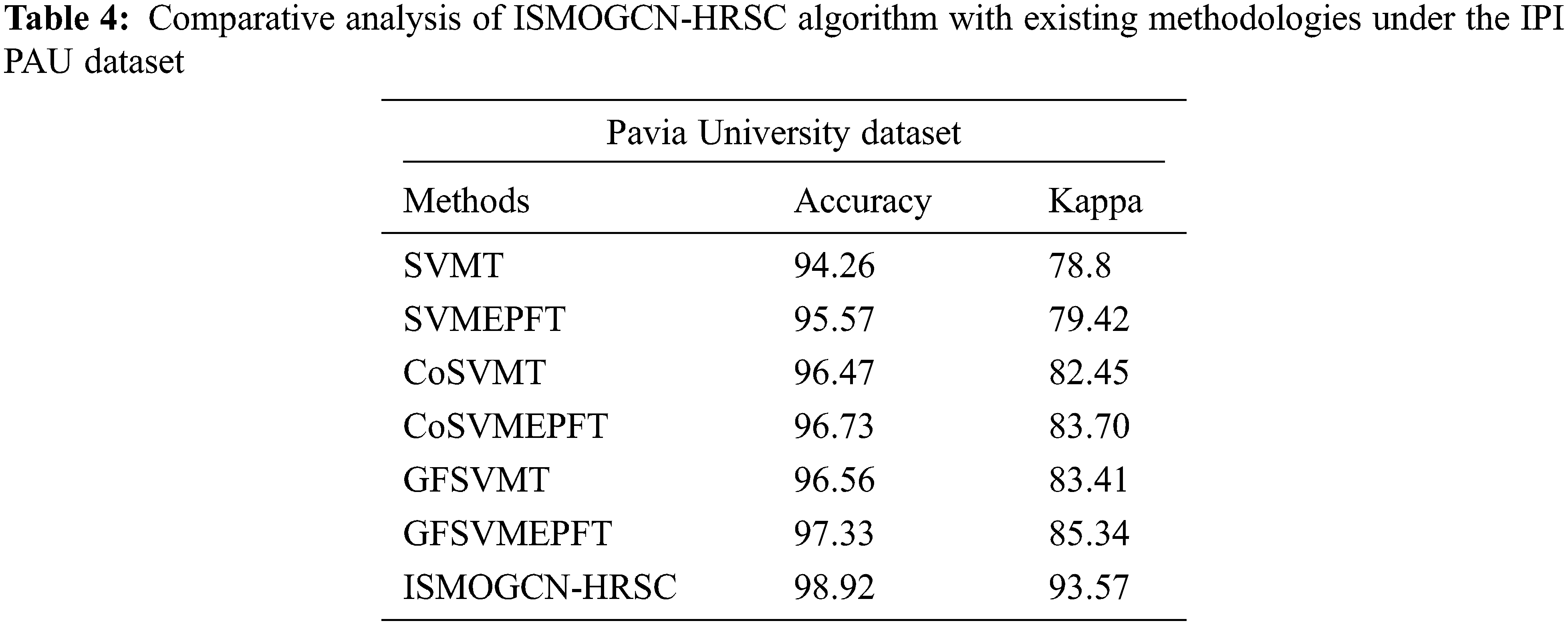
Table 4 demonstrates the comparative outcome of the ISMOGCN-HRSC method with other existing algorithms on the PAU dataset. The outcome exposed that the ISMOGCN-HRSC system has outperformed the improved outcomes of other models. For instance, in terms of accuy , the ISMOGCN-HRSC methodology has attained a higher accuy of 98.92%, whereas the SVMT, SVMEPFT, CoSVMT, CoSVM-EPFT, GFSVMT, and GFSVMEPFT systems have obtained lower accuy of 94.26%, 95.57%, 96.47%, 96.73%. 96.56%, and 97.33% correspondingly. Also, concerning kappa , the ISMOGCN-HRSC algorithm has attained improved kappa of 93.57%, whereas the SVMT, SVMEPFT, CoSVMT, CoSVM-EPFT, GFSVMT, and GFSVMEPFT methodologies have obtained minimal kappa of 78.8%, 79.42%, 82.45%, 83.70%. 83.41% and 85.34%, respectively.

The results mentioned above and the discussion indicated that the ISMOGCN-HRSC model had better performance than compared methods.

5  Conclusion

In this study, a novel ISMOGCN-HRSC approach was presented for identifying and classifying RSIs. The SDL model is exploited in the presented ISMOGCN-HRSC algorithm to produce feature vectors. For image classification purposes, the GCN model is utilized, which enables the identification of the proper class labels of the RSIs. The ISMO algorithm is used to enhance the classification efficacy of the GCN technique, which is derived by integrating chaotic concepts into the SMO algorithm. The experimental assessment of the ISMOGCN-HRSC method was tested using a benchmark dataset. The comparison study reported that the ISMOGCN-HRSC algorithm shows promising performance over other DL techniques that exist in the literature. Thus, the ISMOGCN-HRSC model can be utilized as an effectual RSI classification tool. In the future, the presented ISMOGCN-HRSC approach has been can be extended to the design of hybrid DL-based fusion models to improve the classification performance.

Funding Statement: The authors received no specific funding for this study.

Conflicts of Interest: The authors declare that they have no conflicts of interest to report regarding the present study.

References

    1. J. Song, S. Gao, Y. Zhu and C. Ma, “A survey of remote sensing image classification based on CNNs,” Big Earth Data, vol. 3, no. 3, pp. 232–254, 2019. [Google Scholar]

    2. H. Jiang, M. Peng, Y. Zhong, H. Xie, Z. Hao et al., “A survey on deep learning-based change detection from high-resolution remote sensing images,” Remote Sensing, vol. 14, no. 7, pp. 1552, 2022. [Google Scholar]

    3. A. Sungheetha and R. R. Sharma, “Classification of remote sensing image scenes using double feature extraction hybrid deep learning approach,” Journal of Information Technology and Digital World, vol. 3, no. 2, pp. 133–149, 2021. [Google Scholar]

    4. A. Shakya, M. Biswas and M. Pal, “Parametric study of convolutional neural network based remote sensing image classification,” International Journal of Remote Sensing, vol. 42, no. 7, pp. 2663–2685, 2021. [Google Scholar]

    5. I. Chebbi, N. Mellouli, I. Farah and M. Lamolle, “Big remote sensing image classification based on deep learning extraction features and distributed spark frameworks,” Big Data and Cognitive Computing, vol. 5, no. 2, pp. 21, 2021. [Google Scholar]

    6. F. Özyurt, “Efficient deep feature selection for remote sensing image recognition with fused deep learning architectures,” The Journal of Supercomputing, vol. 76, no. 11, pp. 8413–8431, 2020. [Google Scholar]

    7. S. Liang, J. Cheng and J. Zhang, “Maximum likelihood classification of soil remote sensing image based on deep learning,” Earth Sciences Research Journal, vol. 24, no. 3, pp. 357–365, 2020. [Google Scholar]

    8. X. Li, B. Liu, G. Zheng, Y. Ren, S. Zhang et al., “Deep-learning-based information mining from ocean remote-sensing imagery,” National Science Review, vol. 7, no. 10, pp. 1584–1605, 2020. [Google Scholar]

    9. S. Ullah Khan, I. Ul Haq, N. Khan, K. Muhammad, M. Hijji et al., “Learning to rank: An intelligent system for person reidentification,” International Journal of Intelligent Systems, vol. 37, no. 9, pp. 5924–5948, 2022. [Google Scholar]

  10. N. Dilshad, A. Ullah, J. Kim and J. Seo, “LocateUAV: Unmanned aerial vehicle location estimation via contextual analysis in an IoT environment,” Internet of Things Journal, pp. 1, 2022. Article in press, https://doi.org/10.1109/JIOT.2022.3162300. [Google Scholar]

  11. C. Zhang, G. Li, S. Du, W. Tan and F. Gao, “Three-dimensional densely connected convolutional network for hyperspectral remote sensing image classification,” Journal of Applied Remote Sensing, vol. 13, no. 1, pp. 1, 2019. [Google Scholar]

  12. Y. Bazi, L. Bashmal, M. Rahhal, R. Dayil and N. Ajlan, “Vision transformers for remote sensing image classification,” Remote Sensing, vol. 13, no. 3, pp. 516, 2021. [Google Scholar]

  13. D. Hong, L. Gao, N. Yokoya, J. Yao, J. Chanussot et al., “More diverse means better: Multimodal deep learning meets remote-sensing imagery classification,” IEEE Transactions on Geoscience and Remote Sensing, vol. 59, no. 5, pp. 4340–4354, 2021. [Google Scholar]

  14. N. O. Lynda, N. A. Nnanna and M. M. Boukar, “Remote sensing image classification for land cover mapping in developing countries: a novel deep learning approach,” International Journal of Computer Science & Network Security, vol. 22, no. 2, pp. 214–222, 2022. [Google Scholar]

  15. Y. Li, Y. Zhang and Z. Zhu, “Error-tolerant deep learning for remote sensing image scene classification,” IEEE Transactions on Cybernetics, vol. 51, no. 4, pp. 1756–1768, 2021. [Google Scholar]

  16. J. Xi, O. Ersoy, M. Cong, C. Zhao, W. Qu et al., “Wide and deep fourier neural network for hyperspectral remote sensing image classification,” Remote Sensing, vol. 14, no. 12, pp. 2931, 2022. [Google Scholar]

  17. R. Lei, C. Zhang, W. Liu, L. Zhang, X. Zhang et al., “Hyperspectral remote sensing image classification using deep convolutional capsule network,” IEEE Journal of Selected Topics in Applied Earth Observations and Remote Sensing, vol. 14, pp. 8297–8315, 2021. https://doi.org/10.1109/JSTARS.2021.3101511. [Google Scholar]

  18. Z. Wang, M. K. Ng, L. Zhuang, L. Gao and B. Zhang, “Nonlocal self-similarity-based hyperspectral remote sensing image denoising with 3-D convolutional neural network,” IEEE Transactions on Geoscience and Remote Sensing, vol. 60, pp. 1–17, 2022. https://doi.org/10.1109/TGRS.2022.3182144. [Google Scholar]

  19. X. Dai, X. He, S. Guo, S. Liu, F. Ji et al., “Research on hyper-spectral remote sensing image classification by applying stacked de-noising auto-encoders neural network,” Multimedia Tools and Applications, vol. 80, no. 14, pp. 21219–21239, 2021. [Google Scholar]

  20. N. L. Tun, A. Gavrilov, N. M. Tun, D. M. Trieu and H. Aung, “Hyperspectral remote sensing images classification using fully convolutional neural network,” in 2021 IEEE Conf. of Russian Young Researchers in Electrical and Electronic Engineering (ElConRus), St. Petersburg, Moscow, Russia, pp. 2166–2170, 2021. https://doi.org/10.1109/ElConRus51938.2021.9396673. [Google Scholar]

  21. K. Shankar, E. Perumal, M. Elhoseny, F. Taher, B. Gupta et al., “Synergic deep learning for smart health diagnosis of covid-19 for connected living and smart cities,” ACM Transactions on Internet Technology, vol. 22, no. 3, pp. 1–14, 2022. [Google Scholar]

  22. L. Zhao, Y. Song, C. Zhang, Y. Liu, P. Wang et al., “T-gcn: A temporal graph convolutional network for traffic prediction,” IEEE Transactions on Intelligent Transportation Systems, vol. 21, no. 9, pp. 3848–3858, 2020. [Google Scholar]

  23. K. Sun, H. Jia, Y. Li and Z. Jiang, “Hybrid improved slime mould algorithm with adaptive β hill climbing for numerical optimization,” Journal of Intelligent & Fuzzy Systems, vol. 40, no. 1, pp. 1667–1679, 2021. [Google Scholar]

  24. B. Kuo, H. Ho, C. Li, C. Hung and J. Taur, “A kernel-based feature selection method for SVM with RBF kernel for hyperspectral image classification,” Applied Earth Observations and Remote Sensing, vol. 7, no. 1, pp. 317–326, 2014. [Google Scholar]

  25. F. Luo, B. Du, L. Zhang, L. Zhang and D. Tao, “Feature learning using spatial-spectral hypergraph discriminant analysis for hyperspectral image,” IEEE Transactions on Cybernetics, vol. 49, no. 7, pp. 2406–2419, 2018. [Google Scholar]