Contrastive Clustering for Unsupervised Recognition of Interference Signals

1  Introduction

With the rapid development of wireless communication technology and increased electronic equipment, the future communication system will face more kinds of interference. Adopting corresponding anti-interference methods according to the identified interference signals can improve communication quality. Therefore, interference signals recognition will be one of the critical technologies of intelligent anti-interference communication in the future.

Deep learning has achieved excellent performance in natural language processing [1,2] and computer vision [3–5]. Therefore, many recognition algorithms based on deep learning for interference signals were proposed to solve the problems of traditional interference signal recognition algorithms whose accuracy is low and significantly affected by artificial feature selection [6–12]. However, most interference signals recognition algorithms belong to supervised learning that requires labeled signals samples. Labeling each signal sample requires a lot of labor costs, which limits the applications of these algorithms. Therefore, unsupervised interference signals recognition should study urgently.

Clustering is one of the unsupervised learning methods which can classify data into different clusters without any labeled samples. Traditional clustering methods include partition-based methods, density-based methods, and hierarchy-based methods. In recent years, many unsupervised clustering methods of radio frequency signals have been proposed [13–19]. However, these methods used traditional clustering algorithms and manually selected features. Whether the feature selection is appropriate or not will directly affect its performance. Therefore, without prior knowledge of an interference signal, it is impossible to design artificial features in advance. In addition, the performance of traditional clustering algorithms is poor.

Recently, many deep clustering methods which solve the problems of traditional clustering algorithms have been proposed [20–25], such as semantic clustering by adopting nearest neighbors (SCAN) [24] and contrastive clustering (CC) [25]. Still, these algorithms were used to cluster images, and there is no research on deep clustering for interference signals. On the one hand, the performance of the deep clustering methods with contrastive learning is better than that without it in image clustering. On the other hand, since the interference signal contains noise, the algorithms which used contrastive learning in only one phase will lead to degradation of the noise-immunity caused by data augmentation. Therefore, a method, DDCC, is proposed in this paper. The main contributions can be summarized as follows.

■   To achieve unsupervised interference signals recognition, we propose a method named double phases and double dimensions contrastive clustering. Unlike traditional clustering algorithms, DDCC uses a deep neural network to extract the feature of interference signals automatically.

■   We design four data augmentation strategies for interference signals to carry out DA-based contrastive learning, which is used to pre-train the deep neural network in the first phase of DDCC. In the second phase of DDCC, the KNNset of original data through the pre-trained network is obtained, and the KNNset-based double dimensions contrastive learning is designed to cluster the samples according to their category features. In addition, the stability of DDCC is improved by using a dynamic entropy parameter strategy for regularization.

■   We analyze the performance of the different parts of DDCC through extensive simulation experiments. DDCC, deep embedded clustering (DEC), DeepCluster, deep adaptive clustering (DAC), SCAN, and CC are applied to unsupervised interference signals recognition and compared in experiments. The results show that DDCC outperforms others on unsupervised interference signals recognition under various JNR.

The rest of this paper is organized as follows. Section 2 describes recent work in interference signal recognition based on deep learning and deep clustering. Section 3 discusses the proposed method in detail. Section 4 gives the simulation results and analyzes the performance of different methods in detail. Lastly, Section 5 concludes this paper.

2  Related Work

2.1 Interference Signal Recognition Based on Deep Learning

With the development of deep learning technology, there have been recognition algorithms based on deep learning. The singular value of the signal matrix was used as the input of the multi-layer perceptron (MLP) in [6], and short-time Fourier transform data of jamming signals was used as the input of the convolutional neural network (CNN) in [7,8]. Jamming recognition network [9] based on power spectrum features was proposed to recognize ten kinds of suppression jamming signals. Siamese-CNN [10] and auxiliary classifier variational auto-encoding generative adversarial network [11] were proposed to solve the performance deterioration of the interference signals recognition method in the case of a small sample set. The Auto-Encoder network, which was built by stacking long short-term memory, separated the interference signal from the transmitted signal, and another recurrent neural network realized interference signals recognition [12]. But the above algorithms are supervised, which requires a lot of the labeled signals samples. Deep clustering is one of the unsupervised learning methods.

2.2 Deep Clustering

Deep clustering methods can be divided into two groups. The first group of methods combined traditional clustering algorithms with deep neural networks, such as DEC [20], DeepCluster [21], etc. DEC pre-trained a stacking auto-encoder to obtain the features and used the Kullback-Leibler divergence to jointly train the network and the clustering center obtained by k-means. DeepCluster carried out network training process and k-means clustering alternately. However, their performance can be compromised by the errors accumulated during the traditional clustering. The second group of methods used representation learning and the idea of “label as representation” to solve the problem of the first group of methods, such as DAC [22], invariant information clustering (IIC) [23], SCAN [24], CC [25], etc. DAC used the binary classification with the pseudo label as the pretext task, while IIC used mutual information maximization to realize representation learning. But sometimes, their category features are insufficient to reflect the category relationship between samples. Recently, unsupervised contrastive learning (CL) has achieved state-of-the-art performance in representation learning [26–29]. SCAN and CC that applied contrastive learning to clustering have better clustering performance than DAC and IIC. Because of the high intra-class compactness and inter-class separability of sample features obtained by contrastive learning methods such as simple framework for contrastive learning of visual representations (SIMCLR) [29], SCAN obtained embedding space by using SIMCLR and used the SCAN-loss [24] to make adjacent samples have similar category features. CC performed the instance-level and clustering-level contrastive learning to improve the feature extraction ability of the network and to cluster following the idea of “label as representation”. But SCAN and CC algorithms used contrastive learning only in one phase so that the features extraction network cannot finetune. Moreover, SCAN ignored the inter-class separability of category features, and CC did not utilize the feature distribution explicitly. Therefore the performance of deep clustering for interference signals with noise will deteriorate. Therefore, double phases and double dimensions contrastive clustering for interference signals recognition is proposed to cope with these problems.

3  Double Phases and Double Dimensions Contrastive Clustering

3.1 Data-Augmentation-Based Contrastive Learning

In supervised learning, the feature extraction network training can be guided by sample labels. In contrast, unsupervised learning requires designing pretext-task for network training to enable the network to obtain feature extraction ability, such as rotation prediction [30] and puzzles [31] in image classification. As a promising paradigm of representation learning, contrastive learning is to make the similarity between positive pairs as high as possible and the similarity between negative pairs as low as possible. However, unsupervised learning has no available label to obtain information on positive and negative pairs. Although positive pairs can be obtained by data augmentation that IIC did, the lack of information on negative pairs makes it difficult for features to have inter-class separability.

It is a solution that data augmentation samples from the same sample were considered positive pairs, and that from the different samples were considered negative pairs. Then, the network parameters were updated using the respective contrastive loss functions in [26,27]. Momentum contrast [28] proposed a momentum training approach based on [26], which improves performance in the case of insufficient resources but requires a massive dataset for network training. SIMCLR [29] used a larger batch size, more complex data augmentation strategies, and projection head based on [27], improving the performance without restricting resources. Following SIMCLR, the DA-based contrastive learning is designed in the first phase of DDCC, and the process is shown in Fig. 1.

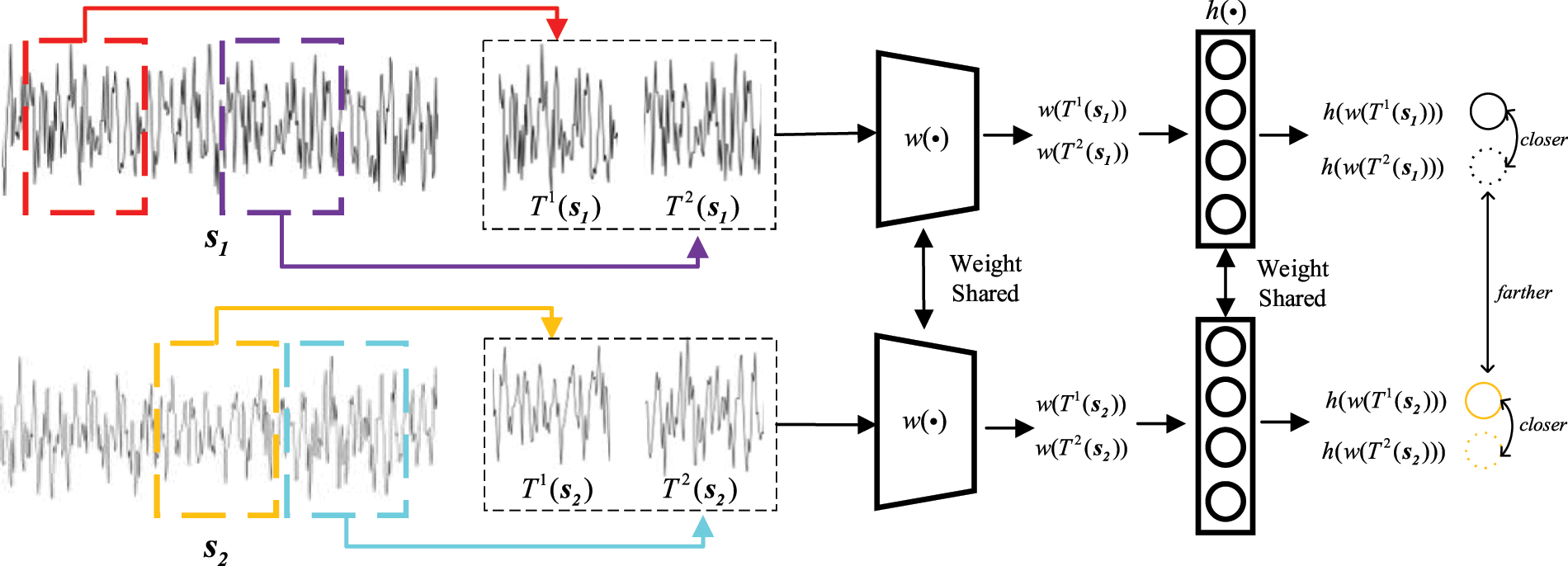
Figure 1: The process of DA-based contrastive learning

Given the unlabeled interference signals dataset D={si}i=1N , where N is the number of samples, si[0], si[1], si[2], … is the sequence of an interference signal. The data augmentation dataset Dnew={T1(si), T2(si)}i=1N is obtained by applying two data augmentation T1 and T2 to all the samples from D. One shared feature extraction network w(⋅) is used to extract the features of the sample from Dnew , and a projection head h(⋅) embeds the features into the Kf dimensional embedding space to get znm=h(w(Tm(sn))) .

The cosine distance between sample features is used to measure the similarity between samples, as shown in Eq. (1),

sim(x, y)=xTy‖x‖‖y‖ (1)

The normalized temperature-scaled cross entropy (NT-Xent) [32] is used as the loss function of DA-based contrastive learning to maximize the similarity of the positive pair while minimizing the similarity of the negative pair, as shown in Eq. (2),

L1=12N∑n=1N[l(zn1, zn2)+l(zn2, zn1)] (2)

where l(x, y)=−logeτsim(x,y)∑m=12∑k=1Neτsim(x,zkm)−1 , τ is the temperature parameter and we let τ=0.5 .

3.2 KNNset-Based Contrastive Learning

In most cases, the nearest neighbors in the embedding space obtained by SIMCLR belong to the same class [24]. Therefore, to enable the network to mine more meaningful semantic information and get better clustering performance, the second phase of DDCC constructs positive and negative pairs according to the KNNset, and performs double dimensions contrastive learning in the feature and the clustering dimension.

3.2.1 Construction of Positive and Negative Pairs

Original samples can provide more meaningful semantic information, so the second phase of DDCC uses KNNset to construct positive and negative pairs while not using data augmentation.

According to the embedding space obtained from contrastive learning in the first phase and cosine distance between samples, KNNset Δk={ηk(si)}i=1N is obtained from the dataset D, where ηk(si) denotes the set of k-nearest neighbors of sample si .

In the training phase, given a batch of samples {si}i=1M , two samples are randomly selected from ηk(s) and two new batches {sia}i=1M and {sib}i=1M are obtained, where sia and sib are selected from ηk(si) , and M is the size of a batch. sia and sib are considered as positive pairs, sia and sjb are considered negative pair, where i≠j .

3.2.2 Double Dimensions Contrastive Learning

As shown in Fig. 2, DDCC performs contrastive learning in the second phase at the feature and clustering dimensions, respectively. The feature dimensional contrastive learning enables the network to extract more meaningful semantic features. In contrast, the clustering dimensional contrastive learning clusters signals through considering category features as the soft assignment probabilities of clusters. Note that, the parameters of w(⋅) and hF(⋅) in the KNNset-based contrastive learning are initialized by the parameters of w(⋅) and h(⋅) in the DA-based contrastive learning, and the parameters of hC(⋅) are initialized randomly.

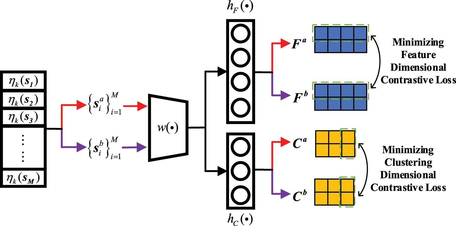
Figure 2: The process of KNNset-based contrastive learning

In the feature dimension, let the feature dimensional outputs of signals sna and snb be fna=hF(w(sna)) and fnb=hF(w(snb)) , respectively, and define the output matrices as Fa=[f1a, f2a, ⋯, fMa]T∈RM×Kf and Fb=[f1b, f2b, ⋯, fMb]T∈RM×Kf , where Kf is feature dimension. And we also utilize the NT-Xent as the loss function of feature dimensional contrastive learning, as shown in Eq. (3),

LF=12M∑n=1M[lF(fna, fnb)+lF(fnb, fna)] (3)

where lF(x, y)=−logeτFsim(x,y)∑n=1MeτFsim(x,fna)+∑n=1MeτFsim(x,fnb)−1 , τF is the temperature parameter and we let τF=0.5 .

In the clustering dimension, a SoftMax layer is added to the end of hC(⋅) to satisfy the probability’s non-negative and sum-to-one properties. Therefore, cna=hC(w(sna)) can be defined the soft assignment probabilities of each cluster of sample sna . The inference process is formulated as:

s∈class arg  ⁡maxi=1KchC(w(s)) (4)

where Kc is the output dimension of the clustering dimensional projection head, i.e., the number of clusters.

Ca=[c1a, c2a, ⋯, cMa]T∈RM×Kc and Cb=[c1b, c2b, ⋯, cMb]T∈RM×Kc are the clustering dimensional output matrices. yia and yib are the ith column of Ca and the ith column of Cb , respectively. So yia and yib can be considered as two representations of the ith cluster. Ideally, yia is equal to yib , and yia is orthogonal to yjb when i≠j . Similar to the feature dimensional contrastive learning, the representations of the same cluster should be similar enough, while the representations of different clusters should be different as much as possible, so the clustering dimensional contrastive learning still uses NT-Xent as loss function:

LC=12Kc∑k=1Kc[lC(yka, ykb)+lC(ykb, yka)] (5)

where lC(x, y)=−logeτCsim(x,y)∑k=1KceτCsim(x,yka)+∑k=1KceτCsim(x,ykb)−1 , τC is the temperature parameter and we let τC=1 .

To avoid the trivial solution caused by assigning nearly all samples to one cluster, we add the entropy term as shown in Eq. (6) for regularization:

LH=−∑n=1Kc[P(yna)log⁡P(yna)+P(ynb)log⁡P(ynb)] (6)

where P(yna)=‖yna‖1/‖Ca‖1 , P(ynb)=‖ynb‖1/‖Cb‖1 .

Finally, to realize the end-to-end training, that is, to update the parameters of the feature extraction network w(⋅) , those of the feature dimensional projection head hF(⋅) and those of the clustering dimensional projection head hC(⋅) at the same time, the hybrid loss function of KNNset-based contrastive learning is defined as:

L2=LF+LC+λLH (7)

where λ is the entropy parameter. A small λ leads to a trivial solution; a large λ can avoid trivial solution but ignores the clustering task of the clustering dimension. Since different datasets may require different λ , we propose a dynamic entropy parameter strategy as shown in Eq. (8):

λ=λmax(0.1×⌈10×eemax⌉) (8)

where λmax and emax are the maximum entropy parameter and the maximum number of iterations, respectively. e is the current epoch, ⌈⋅⌉ denote ceiling operation.

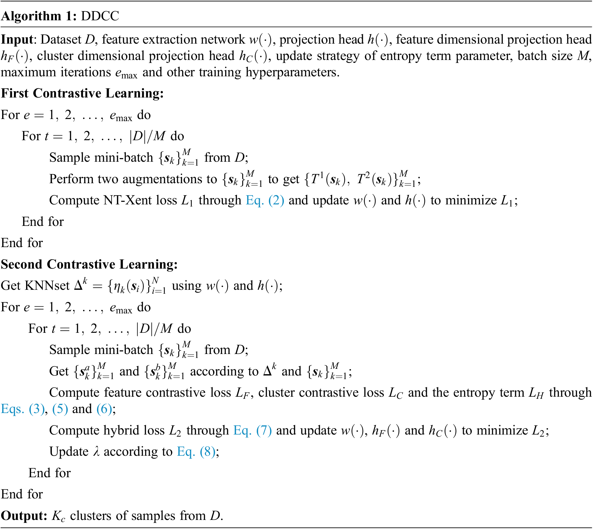
In summary, the entire process of DDCC is shown in Algorithm 1.

4  Performance Analysis

4.1 The Setting of the Experiment

4.1.1 Datasets

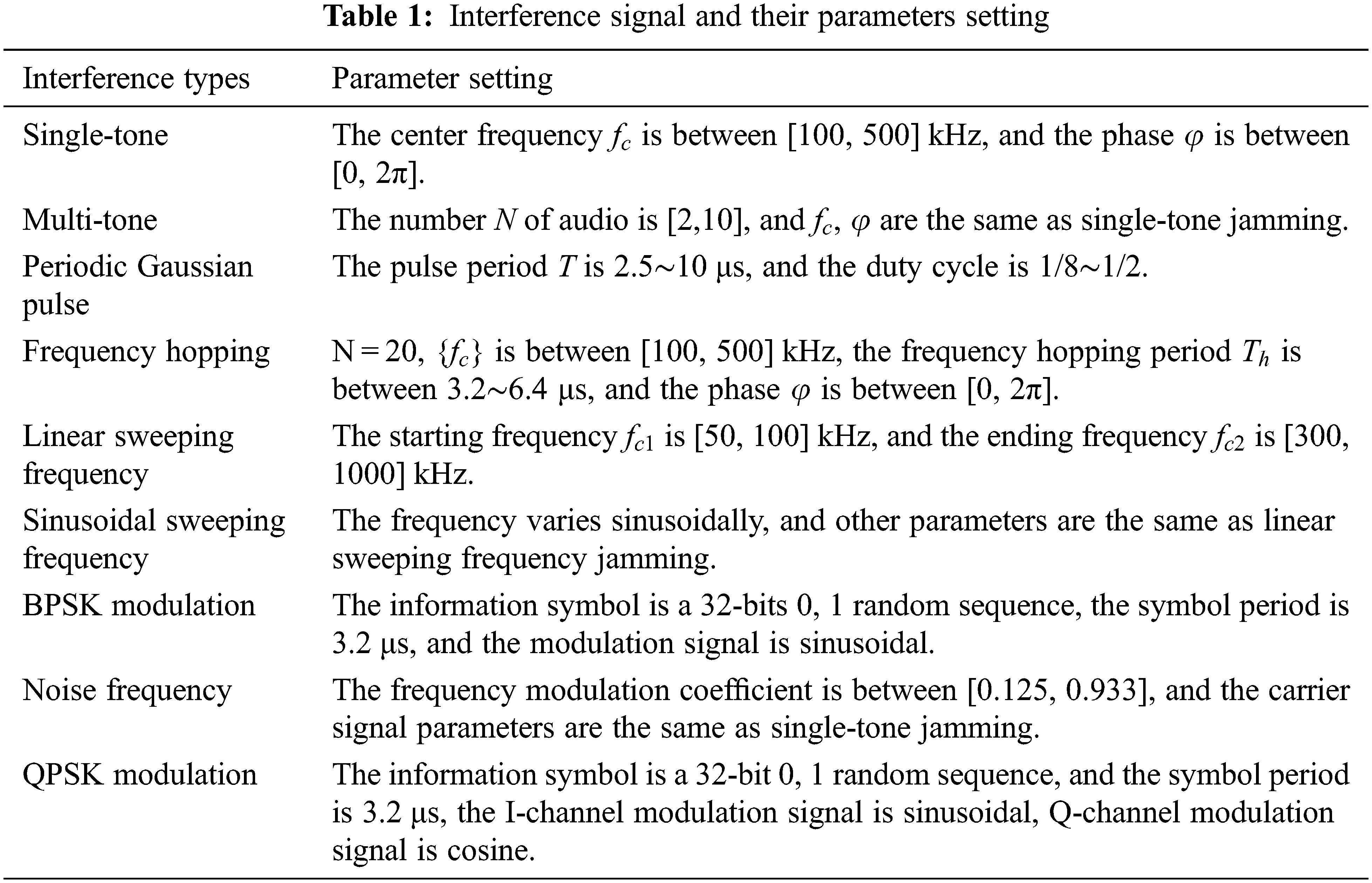
Nine kinds of interference signals, which include single-tone jamming, multi-tone jamming, periodic Gaussian pulse jamming, frequency hopping jamming, linear sweeping frequency jamming, sinusoidal sweeping frequency jamming, binary phase shift keying (BPSK) modulation jamming, noise frequency modulation jamming and quadrature phase shift keying (QPSK) modulation jamming, are generated by matlabR2020a. The details of the parameters of each interference signal are shown in Table 1. The sampling frequency is 10 MHz, and the number of sampling points is 1024. The added noise is additive white Gaussian noise, JNR is −5, 0, 5 and 10 dB, respectively. The number of samples for each category under a JNR is 1000, so there are four datasets with different JNR, and each dataset contains 9000 samples of interference signals.

4.1.2 Network Architecture

We use 1-dimensional densely connected convolutional network [33] as a feature extraction network w(⋅) , and the network used in the first and second phase of DDCC is shown in Fig. 3a. The convolution layer parameter meanings are the convolution kernel’s size, type, number, and stride. For example, {7 conv1d, 32, /2} means the convolution layer uses one-dimensional convolution with 32 convolution kernels whose size is 7 × 1 and stride is 2. For simplicity, we do not draw the batch-normalization layer and rectified linear unit layer before each convolution layer in Fig. 3a. The pooling layer parameter meanings are the pooling kernel’s type, size, and stride. For example, {1dAvgPool, 4, /2} means the pooling layer uses one-dimensional average pooling with a pooling kernel whose size is 4 × 1, and the stride is 2. The fully-connected (FC) layer parameter is the number of the output dimension. The DenseBlock module is shown in Fig. 3b, bn and gr are its parameters of the bottleneck structure and the growth rate, respectively. We set bn=4 , gr=48 . The structure of the transition layer is shown in Fig. 3c, Dimin is the input dimension of the transition layer, and cr is the compression rate of the transition layer which is set to 0.5.

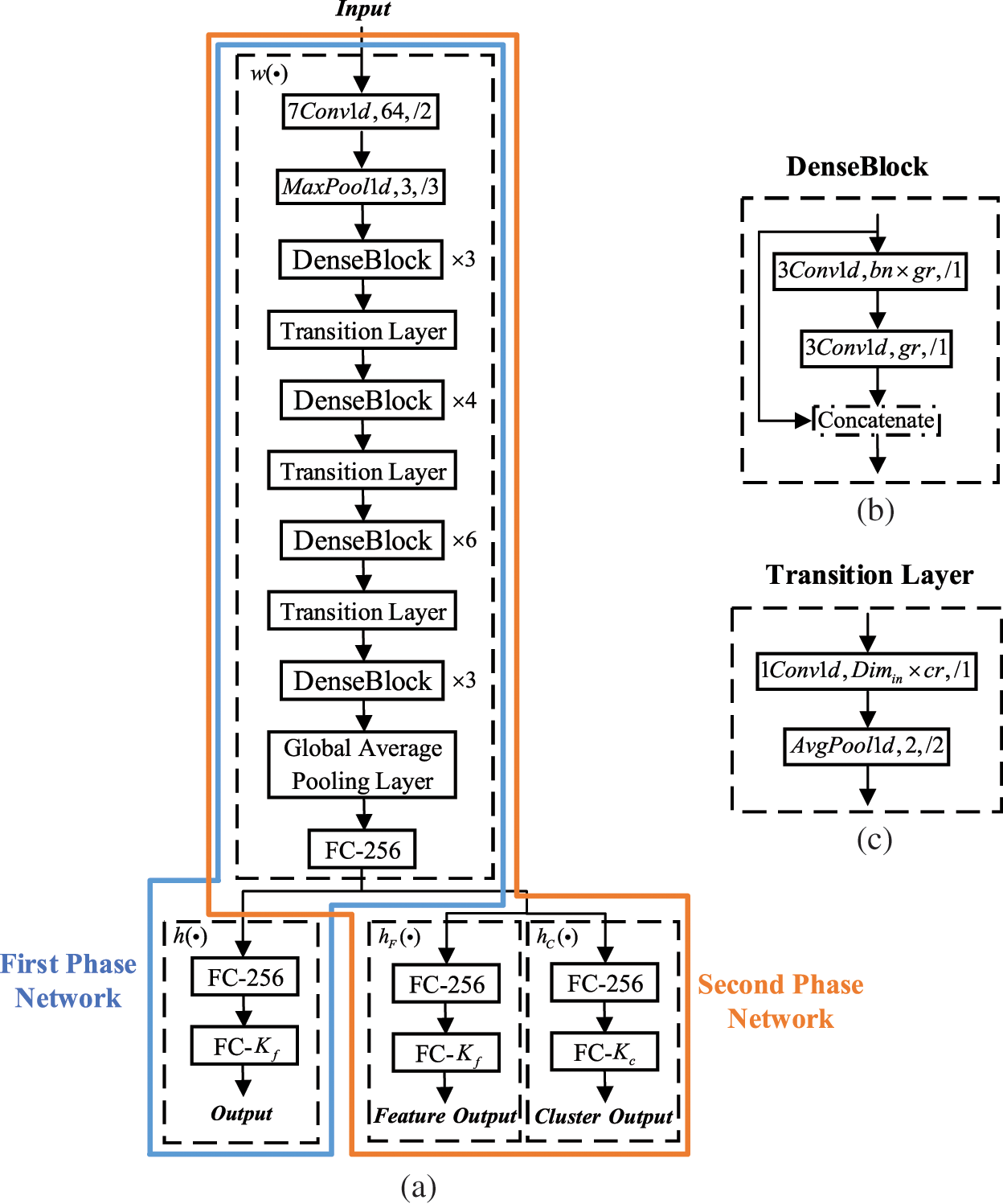
Figure 3: The architectures (a) The network of DDCC; (b) The DenseBlock; (c) The Transition Layer

4.1.3 Training Parameter Setting

During training, the whole network is trained for 120 epochs using the adaptive moment estimate algorithm with 0.0003 learning rate as the optimizer and batch gradient descent with a batch size of 512 as the optimization algorithm. The λmax of dynamic entropy parameter strategy is 0.5.

4.2 Performance Analysis of Data Augmentation Strategies

Four data augmentation strategies, including random cropping, multipath synthesis, down-sampling, and noise injection, to implement DA-based contrastive learning of interference signals, are used and analyzed in this section.

The performance of the data augmentation strategy of the interference signal is measured by the label matching degree (LMD), as shown in Eq. (9):

LMD=1N∑n=1NΛ(ηk(en); en)k (9)

where Λ(ηk(en); en) denotes the number of samples in ηk(en) with labels consistent with en .

The length of random cropping is 256, the number of paths of multipath synthesis is 3, the down-sampling rate is 4, and additive white Gaussian noise with half the power of the original signal is used in noise injection. When k = 20, Kf  = 8 and JNR = −5, 0, 5, and 10 dB, the LMD of different data augmentation strategies are shown in Fig. 4. It can be seen that the LMD of all four strategies increase with the increase of JNR. The LMD of the random cropping strategy is optimal at different JNR. Therefore, random cropping is used as the data augmentation in the following experiments.

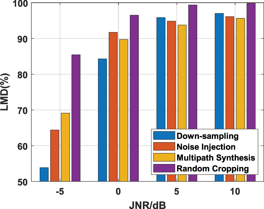
Figure 4: The LMD comparison of contrastive learning using different data augmentation strategies

When JNR is 10 dB, and the random cropping strategy is used with Kf=3 , the 3D scatter plot of the features of the interference signals obtained from the first phase of DDCC is shown in Fig. 5. Note that, because of the normalization, all the samples are projected onto the unit circle. It can be seen that the different types of interference signals have different intra-class compactness and high inter-class separation. So the pre-training method, SIMCLR, can also be applied to the interference signal.

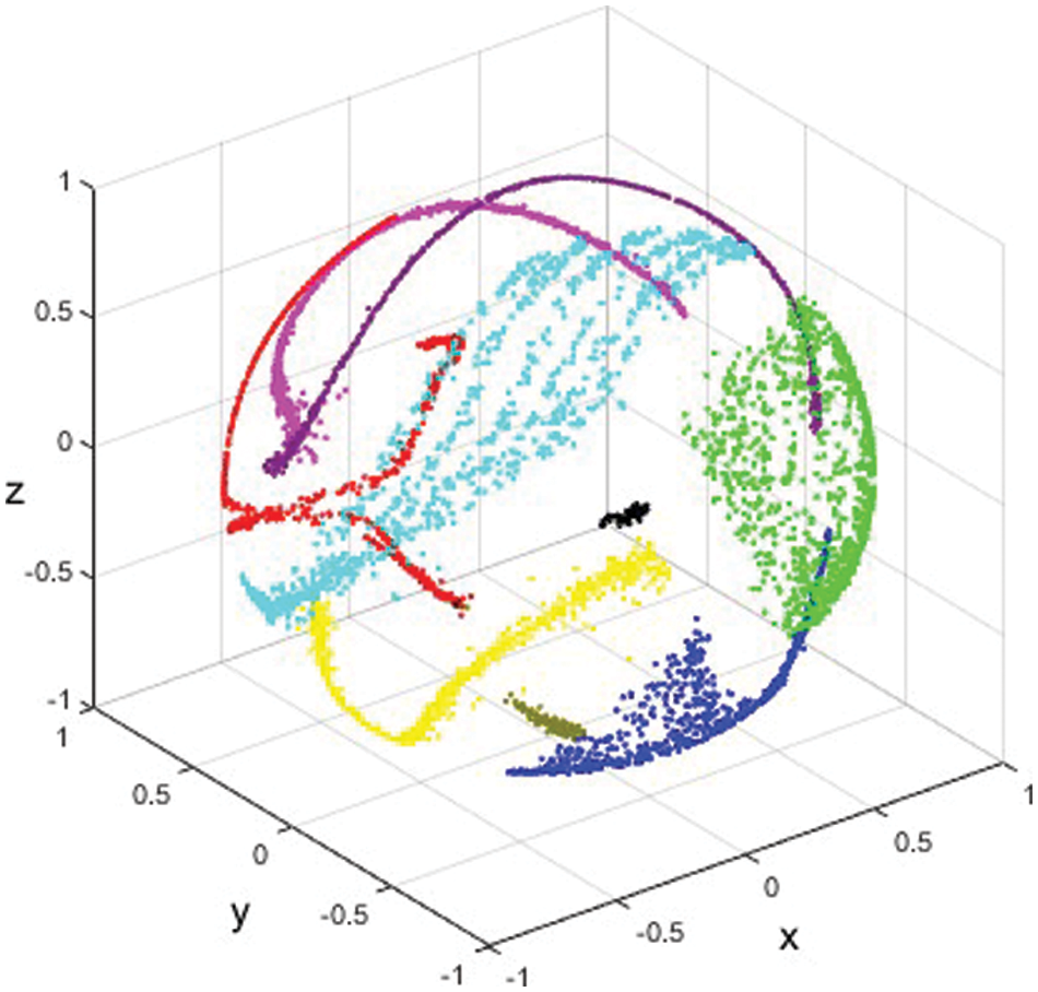
Figure 5: The 3D scatter of signal features in the embedding space

4.3 Effect of the KNNset Selection and Feature Dimensional Contrastive Learning

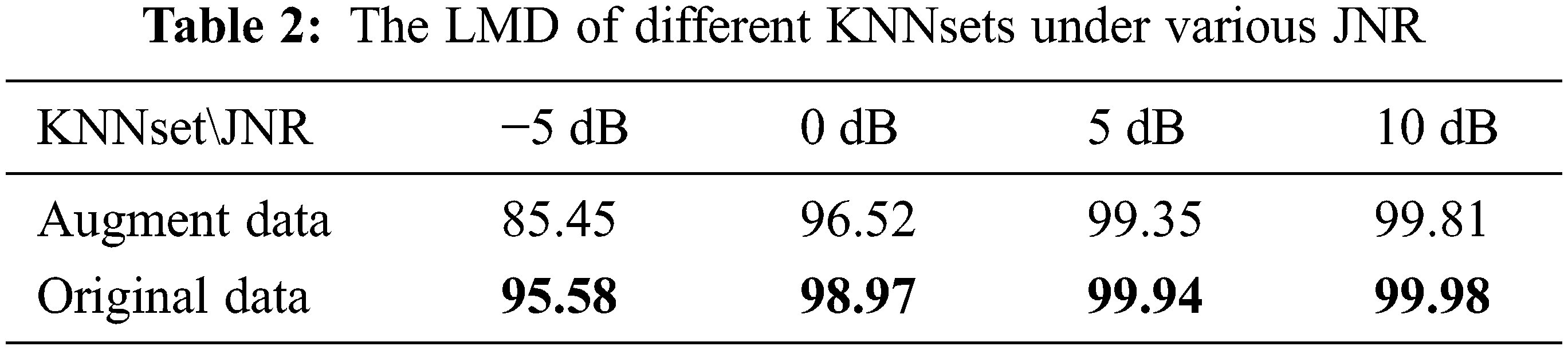
The data augmented and original samples are fed into the pre-training network to obtain the corresponding KNNset. When k = 20, the LMD of two KNNsets with different JNR is shown in Table 2. It can be seen that the LMD of the KNNset obtained according to data augmentation samples decreases significantly when the JNR decreases. In contrast, the LMD of the KNNset obtained according to original samples remains above 95% when JNR is −5 dB. It indicates that although random cropping can obtain excellent LMD of KNNset, it may also lead to losing important information. Since the interference signal contains noise, the data augmentation also affects the noise immunity performance of the algorithm. Therefore, the KNNset is constructed according to original samples and data augmentation is not performed on the KNNset in the second phase.

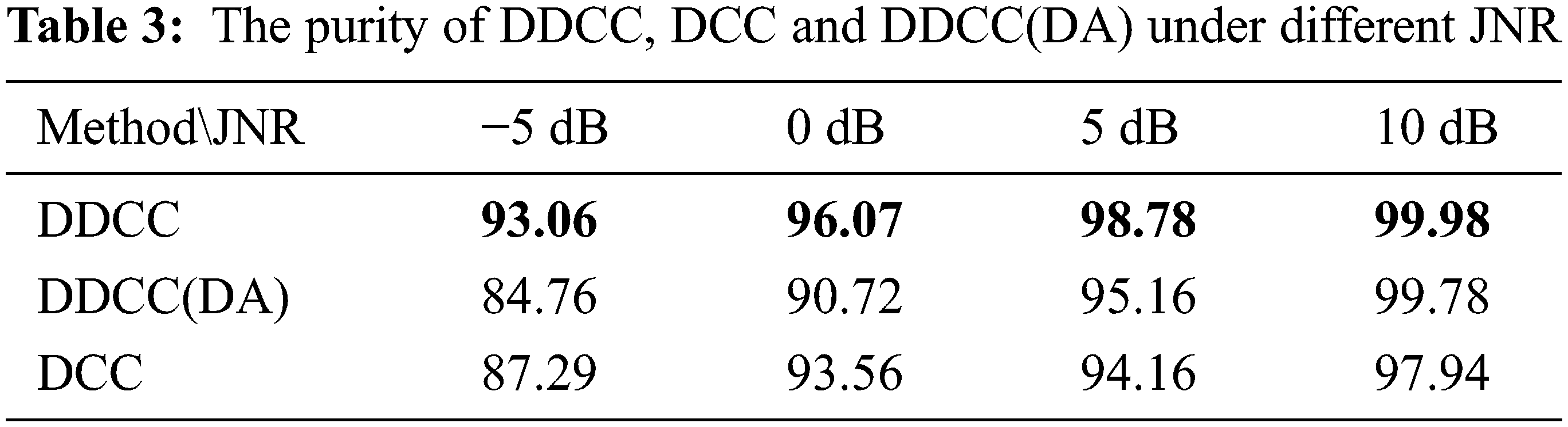
DDCC without using feature dimensional contrastive learning is abbreviated as DCC, and DDCC using data-augmented KNNset is abbreviated as DDCC(DA). The clustering performance of these algorithms is measured using purity, which is defined as Eq. (10):

Purity=1N∑i=1Kcmaxj⁡|pi∩qj| (10)

where N is the number of samples, pi is the set of samples predicted to belong to the ith cluster, qj is the set of samples that belong to the jth class, and |pi∩qj| denotes the total number of samples in the intersection of pi and qj .

The clustering purity of DDCC, DCC, and DDCC(DA) at different JNR is shown in Table 3. We can see that: (1) the purity of DDCC is the highest; the purity of DDCC is higher than that of DCC, indicating that feature dimensional contrastive learning can improve the clustering performance; the purity of DDCC is higher than that of DDCC(DA), indicating that data augmentation to KNNset impairs the noise immunity of DDCC. (2) The purity of DCC is lower than that of DDCC(DA) under 5 dB and 10 dB JNR, and the purity of DCC is better than that of DDCC(DA) under −5 dB and 0 dB JNR, indicating that larger noise power is, more severe degradation of noise immunity performance caused by data augmentation is.

4.4 Effect of Dynamic Entropy Parameter Strategy

Since datasets under various JNR are different and different pre-training networks obtained from the first phase of DDCC lead to different KNNsets, this section analyzes the effect of the dynamic entropy parameter strategy of DDCC.

When the entropy parameter is fixed, the purity curves of DDCC with different pre-training networks under different entropy parameters and JNR are shown in Fig. 6. It can be seen that the optimal parameters are related to the JNR and the pretrained network. When JNR = −5 dB, the optimal entropy parameters of different pretrained networks are 0.15, 0.35 and 0.45, respectively. When JNR = 0 dB, the optimal entropy parameters are 0.1, 0.2 and 0.5, respectively. When JNR = 5 dB, the optimal entropy parameters are 0.15, 0.2 and 0.25, respectively. When JNR = 10 dB, the optimal entropy parameters is 0.05 and 0.15, respectively.

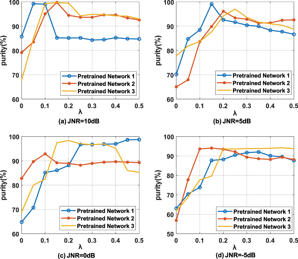
Figure 6: The purity of different pre-trained networks under different JNR using fixed parameter

When using the dynamic entropy parameter strategy, the purity curves of DDCC with different pre-trained networks under different training epoch and JNR are shown in Fig. 7. It can be seen that with the training, the increase of entropy parameter does not cause a significant decrease of purity, and the optimal purity of DDCC with dynamic entropy parameter is higher than that with fixed entropy parameter. In summary, the dynamic entropy parameter strategy proposed in this paper can effectively improve the stability of DDCC.

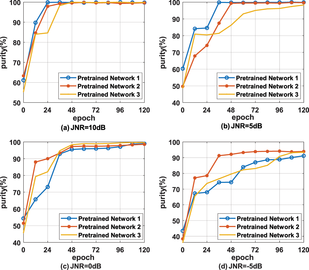
Figure 7: The purity of different pre-trained networks under different JNR using dynamic parameter

4.5 Clustering Performance of Different Methods for Interference Signals

This section applies DDCC, DEC, DeepCluster, DAC, SCAN, and CC to interference signals unsupervised clustering under various JNR. The encoder of DEC, the feature extraction network of DeepCluster, and DAC are the same as the feature extraction network of DDCC. The decoder of DEC reconstructs the original signal through a two-layer FC layer. The network structure of SCAN is the same as the pre-training network of DDCC. The clustering heads of DeepCluster, DAC and SCAN have the same structure as the clustering dimensional projection head of DDCC. The network structure of CC is identical to that of the second phase of DDCC. SCAN, CC, and DDCC all use random cropping as data augmentation. In addition, the performance of the supervised learning method using the cross-entropy loss function is also given. The training set of the unsupervised methods is the test set, and the supervised learning method needs to use an additional test set to evaluate the performance. The purity curves of the seven algorithms under different JNR are shown in Fig. 8. The purity of all methods is the average of the results of 10 random experiments.

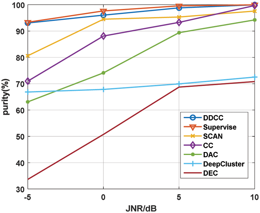
Figure 8: The purity comparison of seven algorithms under different JNR

As can be seen from Fig. 8, the purity of all the algorithms increases with the increase of JNR, and DDCC is the best among the six unsupervised algorithms under different JNR, especially in the low JNR scenario. Under JNR = −5 dB, the purity of DDCC is 12% higher than that of SCAN, which is the suboptimal method. And the purity of DDCC is close to the supervised algorithm when JNR is in the range of −5 to 10 dB. SCAN used SCAN-loss to maintain the intra-class compactness of category features in the second phase, but the loss function ignored their inter-class separability. Unlike SCAN, DDCC uses double dimensional contrastive learning based on KNNset in the second phase, which improves intra-class compactness and inter-class separability of category features and achieves better clustering performance. In addition, the use of the original KNNset makes DDCC have stronger noise immunity. CC used data augmentation samples for double level contrastive learning, which did not explicitly utilize the feature distribution in embedding space obtained by instance-level contrastive learning, and DA-based contrastive learning was not sufficient for obtaining good noise immunity. Unlike CC, DDCC uses KNNset-based contrastive learning, which improves the network feature extraction ability and avoids the problems of information loss and noise immunity degradation caused by data augmentation, as mentioned in Section 4.3. The purity of CC is close to 100% under 10 dB JNR, which is higher than SCAN, but its performance decreases significantly with the decline of JNR.

It also can be seen from Fig. 8 that the purity of the unsupervised algorithms which used contrastive learning is higher than that did not use contrastive learning. The purity of DEC is the worst. DeepCluster performs slightly better than DEC. Still, its clustering purity remains unsatisfactory, while DAC has improved the purity in the JNR range of 0 to 10 dB compared to DeepCluster.

5  Conclusions and Discussion

An unsupervised recognition algorithm of interference signals, double phases and double dimensions contrastive clustering was proposed in this paper. In the first phase, DA-based contrastive learnin was used to pre-train the features extraction network. KNNset-based contrastive learning in the second phase was proposed that used the positive and negative pairs from the KNNset obtained using the distribution of the original signals in the feature space of the pre-trained network. In the second phase, the feature dimensional contrastive learning improved the feature extraction ability of the network by learning the information between the original signals, and the clustering dimensional contrastive learning achieved clustering. Extensive simulation experiments have verified the effectiveness of DDCC. In summary, DDCC has the following characteristics.

DDCC can unsupervised extract more meaningful semantic features and more accurate category features. Simulation results showed the unsupervised recognition performance of DDCC for nine interference signals is better than the other unsupervised clustering algorithms and close to the supervised learning algorithm in the JNR range of −5 to 10 dB.

Random cropping is the best strategy among the four data augmentation strategies in the first phase of DDCC. The double dimensions contrastive learning in the second phase, which uses the KNNset and hybrid loss function, can fine-tune the feature extraction network and cluster more accurately and steadily. Simulation results validated the high clustering purity of DDCC under low JNR and the stability of DDCC. But DDCC needs to know the cluster number in advance like the other deep clustering method.

In future work, open-world recognition of interference signals will be achieved by combining open-set recognition and incremental learning.

Funding Statement: This research was supported by the National Natural Science Foundation of China under Grant No. U19B2016., and Zhejiang Provincial Key Lab of Data Storage and Transmission Technology, Hangzhou Dianzi University.

Conflicts of Interest: The authors declare that they have no conflicts of interest to report regarding the present study.

References

    1. M. Anwar Hussen Wadud, M. F. Mridha, J. Shin, K. Nur and A. Kumar Saha, “Deep-bert: Transfer learning for classifying multilingual offensive texts on social media,” Computer Systems Science and Engineering, vol. 44, no. 2, pp. 1775–1791, 2023. [Google Scholar]

    2. A. R. W. Sait and M. K. Ishak, “Deep learning with natural language processing enabled sentimental analysis on sarcasm classification,” Computer Systems Science and Engineering, vol. 44, no. 3, pp. 2553–2567, 2023. [Google Scholar]

    3. A. S. Almasoud, “Intelligent deep learning enabled wild forest fire detection system,” Computer Systems Science and Engineering, vol. 44, no. 2, pp. 1485–1498, 2023. [Google Scholar]

    4. R. Punithavathi, A. D. C. Rani, K. R. Sughashini, C. Kurangi, M. Nirmala et al., “Computer vision and deep learning-enabled weed detection model for precision agriculture,” Computer Systems Science and Engineering, vol. 44, no. 3, pp. 2759–2774, 2023. [Google Scholar]

    5. K. Bayoudh, R. Knani, F. Hamdaoui and A. Mtibaa, “A survey on deep multimodal learning for computer vision: Advances, trends, applications, and datasets,” Visual Computer, vol. 38, no. 8, pp. 2939–2970, 2022. [Google Scholar]

    6. M. Feng and Z. Wang, “Interference recognition based on singular value decomposition and neural network,” Journal of Electronics & Information Technology, vol. 42, no. 11, pp. 2573–2578, 2020. [Google Scholar]

    7. Y. Wang, B. Sun and N. Wang, “Recognition of radar active-jamming through convolutional neural networks,” The Journal of Engineering, vol. 2019, no. 21, pp. 7695–7697, 2019. [Google Scholar]

    8. Q. Liu and W. Zhang, “Deep learning and recognition of radar jamming based on CNN,” in Proc. ISCID, Hangzhou, China, pp. 208–212, 2019. [Google Scholar]

    9. Q. Qu, S. Wei, S. Liu, J. Liang and J. Shi, “JRNet: Jamming recognition networks for radar compound suppression jamming signals,” IEEE Transactions on Vehicular Technology, vol. 69, no. 12, pp. 15035–15045, 2020. [Google Scholar]

  10. G. Shao, Y. Chen and Y. Wei, “Convolutional neural network-based radar jamming signal classification with sufficient and limited samples,” IEEE Access, vol. 8, pp. 80588–80598, 2020. [Google Scholar]

  11. Y. Tang, Z. Zhao, X. Ye, S. Zheng and L. Wang, “Jamming recognition based on AC-VAEGAN,” in Proc. ICSP, Beijing, China, pp. 312–315, 2020. [Google Scholar]

  12. Q. Wu, Z. Sun and X. Zhou, “Interference detection and recognition based on signal reconstruction using recurrent neural network,” in Proc. GC Wrokshop, Hawaii Big Island, USA, pp. 1–6, 2019. [Google Scholar]

  13. T. C. Clancy, A. Khawar and T. R. Newman, “Robust signal classification using unsupervised learning,” IEEE Transactions on Wireless Communications, vol. 10, no. 4, pp. 1289–1299, 2011. [Google Scholar]

  14. G. Zhang, X. Yan, S. Wang and Q. Wang, “A novel automatic modulation classification for M-QAM signals using adaptive fuzzy clustering model,” in Proc. ICCWAMTIP, Chengdu, China, pp. 45–48, 2018. [Google Scholar]

  15. F. Yang, L. Yang, D. Wang, P. Qi and H. Wang, “Method of modulation recognition based on combination algorithm of K-means clustering and grading training SVM,” China Communications, vol. 15, no. 12, pp. 55–63, 2018. [Google Scholar]

  16. J. Norolahi, M. Mehrnia and P. Azmi, “Blind modulation classification via combined machine learning and signal feature extraction,” in Proc. ISMODE, Jakarta, Indonesia, pp. 266–271, 2022. [Google Scholar]

  17. G. Jajoo, Y. K. Yadav and S. Yadav, “Blind signal digital modulation classification through k-medoids clustering,” in Proc. ANTS, Indore, India, pp. 1–5, 2018. [Google Scholar]

  18. J. Mouton, M. Ferreira and A. Helberg, “A comparison of clustering algorithms for automatic modulation classification,” Expert Systems with Applications, vol. 151, pp. 113317, 2020. [Google Scholar]

  19. L. Liu and S. Xu, “Unsupervised radar signal recognition based on multi-block multi-view low-rank sparse subspace clustering,” IET Radar Sonar and Navigation, vol. 16, no. 3, pp. 542–551, 2018. [Google Scholar]

  20. J. Xie, R. Girshick and A. Farhadi, “Unsupervised deep embedding for clustering analysis,” in Proc. ICML, New York City, USA, pp. 478–487, 2016. [Google Scholar]

  21. M. Caron, P. Bojanowski, A. Joulin and M. Douze, “Deep clustering for unsupervised learning of visual features,” in Proc. ECCV, Munich, Germany, pp. 139–156, 2018. [Google Scholar]

  22. J. Chang, L. Wang, G. Meng, S. Xiang and C. Pan, “Deep adaptive image clustering,” in Proc. ICCV, Venice, Italy, pp. 5880–5888, 2017. [Google Scholar]

  23. X. Ji, J. Henriques and A. Vedaldi, “Invariant information clustering for unsupervised image classification and segmentation,” in Proc. ICCV, Seoul, Korea, pp. 9864–9873, 2019. [Google Scholar]

  24. W. V. Gansbeke, S. Vandenhende, S. Georgoulis, M. Proesmans and L. V. Gool, “SCAN: Learning to classify images without labels,” in Proc. ECCV, Glasgow, UK, pp. 268–285, 2020. [Google Scholar]

  25. Y. Li, P. Hu, Z. Liu, D. Peng, J. T. Zhou et al., “Contrastive clustering,” in Proc. AAAI, Vancouver, Canada, pp. 8547–8555, 2021. [Google Scholar]

  26. Z. Wu, Y. Xiong, S. X. Yu and D. Lin, “Unsupervised feature learning via non-parametric instance discrimination,” in Proc. CVPR, Salt Lake City, USA, pp. 3733–3742, 2018. [Google Scholar]

  27. M. Ye, X. Zhang, P. C. Yuen and S. Chang, “Unsupervised embedding learning via invariant and spreading instance feature,” in Proc. CVPR, Long Beach, CA, USA, pp. 6203–6212, 2019. [Google Scholar]

  28. K. He, H. Fan, Y. Wu, S. Xie and R. Girshick, “Momentum contrast for unsupervised visual representation learning,” in Proc. CVPR, Seattle, USA, pp. 9726–9735, 2020. [Google Scholar]

  29. T. Chen, S. Kornblith, M. Norouzi and G. Hinton, “A simple framework for contrastive learning of visual representations,” in Proc. ICML, Seattle, USA, pp. 1597–1607, 2020. [Google Scholar]

  30. S. Gidaris, P. Singh and N. Komodakis, “Unsupervised representation learning by predicting image rotations,’’ 2018. [Online]. Available: https://arxiv.org/abs/1803.07728. [Google Scholar]

  31. C. Wei, L. Xie, X. Ren, Y. Xia, C. Su et al., “Iterative reorganization with weak spatial constraints: Solving arbitrary jigsaw puzzles for unsupervised representation learning,” in Proc. CVPR, Long Beach, USA, pp. 1910–1919, 2019. [Google Scholar]

  32. K. Sohn, “Improved deep metric learning with multi-class n-pair loss objective,” in Proc. NeurIPS, Barcelona, Spain, pp. 1857–1865, 2016. [Google Scholar]

  33. G. Huang, Z. Liu, L. Maaten and K. Q. Weinberger, “Densely connected convolutional networks,” in Proc. CVPR, Honolulu, USA, pp. 2261–2269, 2017. [Google Scholar]