
 Submit a Paper
 Propose a Special lssue
 Open Access
ARTICLE

Earthworm Optimization with Improved SqueezeNet Enabled Facial Expression Recognition Model
1 Computer Science and Engineering Department, Gayatri Vidya Parishad College of Engineering for Women, Visakhapatnam, Andhra Pradesh, India
2 Department of Software Engineering, College of Computer Science and Engineering, University of Jeddah, Jeddah, Saudi Arabia
3 King Abdul Aziz City for Science and Technology, Riyadh, Kingdom of Saudi Arabia
4 Department of Computer Science and Engineering, Vignan’s Institute of Information Technology, Visakhapatnam, 530049, India
5 School of Electrical and Electronic Engineering, Engineering Campus, Universiti Sains Malaysia (USM), Nibong Tebal, Penang, 14300, Malaysia
6 Department of Information Systems, College of Computer and Information Sciences, Princess Nourah bint Abdulrahman University, Saudi Arabia
7 Department of Computer Science, University of Central Asia, Naryn, 722600, Kyrgyzstan
8 Faculty of Computers and Information, South Valley University, Qena, 83523, Egypt
* Corresponding Author: Hend Khalid Alkahtani. Email:
Computer Systems Science and Engineering 2023, 46(2), 2247-2262. https://doi.org/10.32604/csse.2023.036377
Received 28 September 2022; Accepted 08 December 2022; Issue published 09 February 2023
 View Full Text
 Download PDF
Abstract
Facial expression recognition (FER) remains a hot research area among computer vision researchers and still becomes a challenge because of high intra-class variations. Conventional techniques for this problem depend on hand-crafted features, namely, LBP, SIFT, and HOG, along with that a classifier trained on a database of videos or images. Many execute perform well on image datasets captured in a controlled condition; however not perform well in the more challenging dataset, which has partial faces and image variation. Recently, many studies presented an endwise structure for facial expression recognition by utilizing DL methods. Therefore, this study develops an earthworm optimization with an improved SqueezeNet-based FER (EWOISN-FER) model. The presented EWOISN-FER model primarily applies the contrast-limited adaptive histogram equalization (CLAHE) technique as a pre-processing step. In addition, the improved SqueezeNet model is exploited to derive an optimal set of feature vectors, and the hyperparameter tuning process is performed by the stochastic gradient boosting (SGB) model. Finally, EWO with sparse autoencoder (SAE) is employed for the FER process, and the EWO algorithm appropriately chooses the SAE parameters. A wide-ranging experimental analysis is carried out to examine the performance of the proposed model. The experimental outcomes indicate the supremacy of the presented EWOISN-FER technique.Keywords
Facial expression recognition (FER) plays a pivotal role in the artificial intelligence (AI) period. Following the emotional information of humans, machines could offer personalized services. Several applications, namely customer satisfaction, virtual reality, personalized recommendations, and many more, rely upon an effective and dependable way of recognizing facial expressions [1]. This topic has grabbed the attention of several research scholars for years. Still, it becomes a challenging topic as expression features change significantly with environments, head poses, and discrepancies in the different individuals involved [2]. Technologies for transmission have conventionally been formulated based on the senses that serve as the main part of human communication. Specifically, AI voice recognition technology utilizing AI speakers and sense of hearing was commercialized due to the enhancements in AI technology [3]. By using this technology that identifies voice and language, there are AI robots that could communicate thoroughly with real life for handling the daily lists of individuals. But sensory acceptance was needed to communicate more accurately [4]. Thus, the most essential technology was a vision sensor, since vision becomes a large part of human perception in many communications.
AI robots communicate between a machine and a human, human faces present significant data as a hint to understand the user’s present state. Thus, the domain of FER has been studied broadly for the past 10 years [5]. Currently, with the rise of appropriate data and continuous progression of deep learning (DL), a FER mechanism that precisely identifies facial expressions in several surroundings is being studied actively [6]. FER depends on an evolutionary and ergonomic technique. Depending on physiological and evolutionary properties, universality, similarity, and emotions in FER research are categorized into 6 categories: anger, happiness, disgust, sadness, surprise, and fear [7]. Moreover, emotions are further categorized into 7 categories, along with neutral emotion. Motivated by the achievement of Convolutional Neural Networks (CNNs), numerous existing DL techniques were devised for facial expression recognition and were superior to conventional techniques. CNN-related techniques could automatically learn and model the extracted features of the facial object due to the neural network structure; therefore, such methods could have superior outcomes in real-time applications [8]. In recent times, by using DL and particularly CNNs, numerous features have been learned and extracted for a decent FER mechanism [9]. It is noted that, in facial expressions, several clues arise from some parts of the face, for example, the eyes and mouth; other parts, like the hair and ears, play little parts in the result [10]. This indicates that the machine learning (ML) structure preferably must concentrate only on significant parts of the face and be less delicate than other facial areas.
This study develops an earthworm optimization with an improved SqueezeNet-based FER (EWOISN-FER) model. The presented EWOISN-FER model primarily applies contrast limited adaptive histogram equalization (CLAHE) technique as a pre-processing step. In addition, the improved SqueezeNet model is exploited to derive an optimal set of feature vectors, and the stochastic gradient boosting (SGB) model performs the hyperparameter tuning process. Finally, EWO with sparse autoencoder (SAE) is employed for the FER process, and the EWO algorithm appropriately chooses the SAE parameters. A wide-ranging experimental analysis is carried out to demonstrate the enhanced performance of the EWOISN-FER technique.
The remaining sections of the paper are organized as follows. Section 2 provides the literature review, and Section 3 elaborates on the proposed model. Then, Section 4 offers performance validation, and Section 5 concludes.
Nezami et al. [11] introduced a DL algorithm for improving engagement recognition from images that overwhelm the challenges of data sparsity via pre-training on an easily accessible facial expression dataset and beforehand training on a specialized engagement dataset. Firstly, FER can be trained to give a rich face representation using DL. Next, the model weight is employed for initializing the DL-based methodology for recognizing engagement; we term this the engagement module. Bargshady et al. [12] report on a newly improved DNN architecture intended to efficiently diagnose pain intensity in 4-level thresholds with facial expression images. To examine the robustness of presented techniques, the UNBC-McMaster Shoulder Pain Archive Database contains facial images of humans and has been first balanced after being utilized for testing and training the classifier technique, in addition, to optimally tuning the VGG-Face pre-trainer as a feature extracting tool. The pre-screened attributes, utilized as method inputs, were transmitted to generate a novel enhanced joint hybrid CNN-BiLSTM (EJH-CNN-BiLSTM) DL technique that encompasses CNN, which can be linked to the joint Bi-LSTM for multi-classifying the pain.
The authors in [13] concentrate on a semi-supervised deep belief network (DBN) method for predicting facial expressions. To achieve precise facial expression classification, a gravitational search algorithm (GSA) was applied to optimise certain variables in the DBN network. The HOG features derived from the lip patch offer optimal performance for precise facial expression classification. In [14], a new deep model can be presented to enhance facial expressions’ classifier accuracy. The presented method includes the following merits: initially, a pose-guided face alignment technique was presented to minimize the intra-class modification surpassing environmental noise’s effect. A hybrid feature representation technique has been presented to gain high-level discriminatory facial features that attain superior outcomes in classifier networks. A lightweight fusion backbone was devised that integrates the ResNet and the VGG-16 to obtain low-data and low-calculation training.
Minaee et al. [15] modelled a DL technique related to attentional convolutional networks to focus on significant face areas and attain important enhancement over prior methods on many datasets. Kim et al. [16] present a novel FER mechanism related to the hierarchical DL technique. The feature derived from the appearance feature-oriented network can be merged with the geometric feature in a hierarchical framework. The presented technique integrates the outcome of the softmax function of 2 features by considering the mistake linked with the second highest emotion (Top-2) predictive outcome. Further, the author presents a method for generating facial imageries with neutral emotion utilizing the autoencoder (AE) method. By this method, the author could derive the dynamic facial features among the emotional and neutral images without sequence data.
In this study, a new EWOISN-FER algorithm was devised to recognise and classify facial emotions. The presented EWOISN-FER model employed the CLAHE technique as a pre-processing step. In addition, an improved SqueezeNet method is exploited to derive an optimal set of feature vectors, and the SGB model performs the hyperparameter tuning process. Lastly, EWO with SAE is employed for the FER process and the EWO algorithm appropriately chooses the SAE parameters. Fig. 1 demonstrates the block diagram of the EWOISN-FER algorithm.
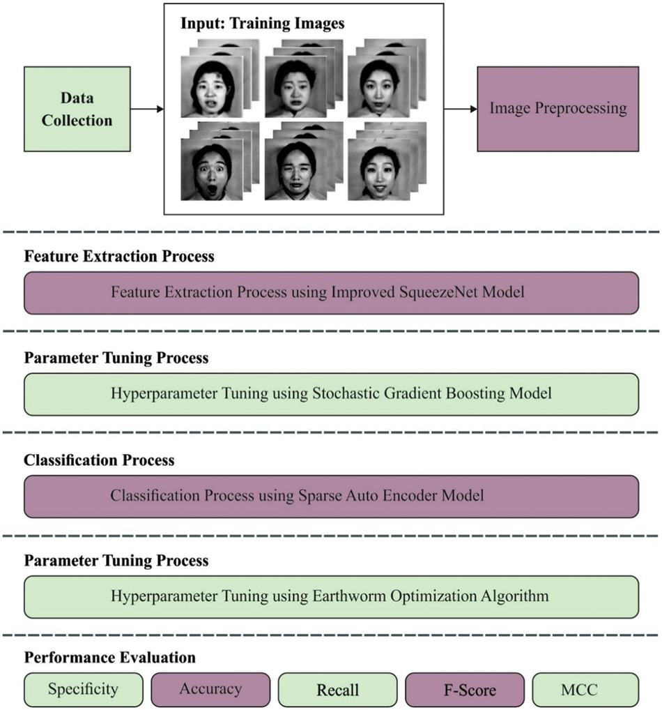
Figure 1: Block diagram of EWOISN-FER approach
CLAHE splits the image into MxN local tiles. For all the tiles, histograms can be individually calculated [17]. First, we should compute the average amount of pixels for each region to computer the histogram as follows:
Here,
N
where
The overall amount of clipped pixels is calculated by the following equation.
Let,
Now,
The amount of undistributed pixels is calculated using Eqs. (4) and (5). Eq. (6) is repeated until each pixel is redistributed. Lastly, the cumulative histogram of the context region is formulated as follows.
After each calculation is accomplished, the histogram of the contextual region is matched with Rayleigh, exponential or uniform likelihood distribution. For the output image, the tile is fused and the removal of the artefacts among the independent tiles is completed using the bilinear interpolation, the novel value of s that is represented by
Then, the enhanced image is attained.
3.2 Feature Extraction Using Improved SqueezeNet
In this stage, the improved SqueezeNet method is exploited to derive an optimal set of feature vectors, and the hyperparameter tuning process can be performed by the SGB model. The CNN initiates with a standalone convolutional layer (conv1) and slowly increases the filter number for all the fire modules from the start to the end of the networks. The CNN architecture implements max pool with a stride of 2 afterwards layers conv1, fire4, fire8, and conv10. Since the light weighted SqueezeNet architecture trained on the insect databases with 9 object classes, we adapted the conv10 layers (because they are personalized to other tasks) that comes from the pre-trained SqueezeNet CNN architecture and replaces newly adapted conv10 layers with a nine-class output [18]. In this study, the Fire module contains 1 × 1 filter
Furthermore, a bypass connection is added to improve the representation bottleneck presented by squeeze layers, however, the limitation is that the quantity of input channels of the Fire module and amount of output channels is dissimilar, and the component-wise addition operator could not be satisfied. Hence, determine a complicated bypass as a bypass that involves a 1 × 1 convolutional layer with the number of filters equal to the number of output channels. In such a way, we require the module for learning a residual function among inputs and outputs, in the meantime, attaining the upper convolutional layer with rich semantic data. Fig. 2 illustrates the architecture of SqueezeNet. The experiment result shows the best object detection performance compared to the pre-trained, light-weighted SqueezeNet CNN module. The final softmax layers frequently handle multi-classification problems. In softmax regression, the probability p that an input ×belonging to class c is formulated below
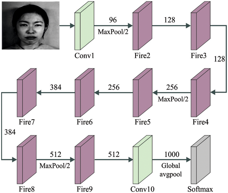
Figure 2: Structure of SqueezeNet
In Eq. (9),
In Eq. (10), 1 signifies an indicative function whose value is 1 as long as the
Friedman [19] built an SGB model by presenting the concept of gradient descent (GD) into the boosting algorithm. Gradient boosting is an ensemble learning mechanism fused with the decision and boosting trees, and the novel paradigm is constructed alongside the GD direction of the loss function of the predetermined method. The core of the SGB approach is to minimalize the loss function among the classification and real functions by training the classifier function
The loss function distribution is the core element of the application of the SGB algorithm, and it has pertinence towards each loss function. For the K-class problem, the substitute loss function (multiclass
Now
In Eq. (12),
Every function is upgraded and later established as the SGB.
3.3 FER Process Using Optimal SAE
At the final stage, the SAE model is employed for FER. During this case, it can execute the hyperbolic tangent activation function to encode and decode [21]. Primarily, the bias vector and weight matrix were allocated arbitrary values. For obtaining a network with generalized ability, the number of trained instances is at least 10 times the count of degrees of the freedoms. The recreated errors decreased significantly with training for determining suitable values of weight and bias. Utilizing the sparse AE, the cost function signifies the reconstructed errors demonstrated in Eq. (14).
whereas E signifies the cost function of AE; N denotes the number of trained instances, K refers to the dimensional of data;
To improve AE’s generation capability and avoid overfitting, the
In which C indicates the count of hidden layers and
whereas
The EWO algorithm is exploited in this study to adjust the SAE parameters. The EWO algorithm was exploited that is simulated the reproductive process of earthworms (EW) to overcome the optimization problems [22]. The EW is a kind of hermaphrodite and performs at all of them and employs female and male sex organs. Consequently, the single parent EW produces a child EW via themselves:
The abovementioned equation described the process of producing
The Reproduction_2 applies an enhanced kind of crossover operator. Consider M as the number of child EWs, which is 2 or 3 in major components. The amount of parent EWs (N) is an integer that is greater than 1. In the study, the uniform crossover was employed with
Firstly, 2 offspring
If
Then,
Finally, the produced EW
Then, the producing EWs
In Eq. (25),
Now,
In Eq. (27),
Now,
The EWO technique mostly defines a fitness value to accomplish maximal classification outcomes. It calculates a positive integer for demonstrating enhanced outcomes on the candidate solution. In the study, decreasing the classification error rate could be processed as the fitness function, as follows. The optimal holds the least error rate, and the poorly attained solution provides a higher error rate.
The FER performance of the EWOISN-FER model is tested using two datasets namely CK+ [23] and RaFD [24] datasets. The CK+ dataset holds 630 samples under seven classes, and the RaFD dataset comprises 3377 samples under seven classes, as depicted in Table 1. A few sample images are displayed in Fig. 3. Fig. 4 indicates the confusion matrices of the EWOISN-FER model on CK+ dataset. The confusion matrices demonstrated that the EWOISN-FER model can effectually recognize seven distinct types of facial expressions.
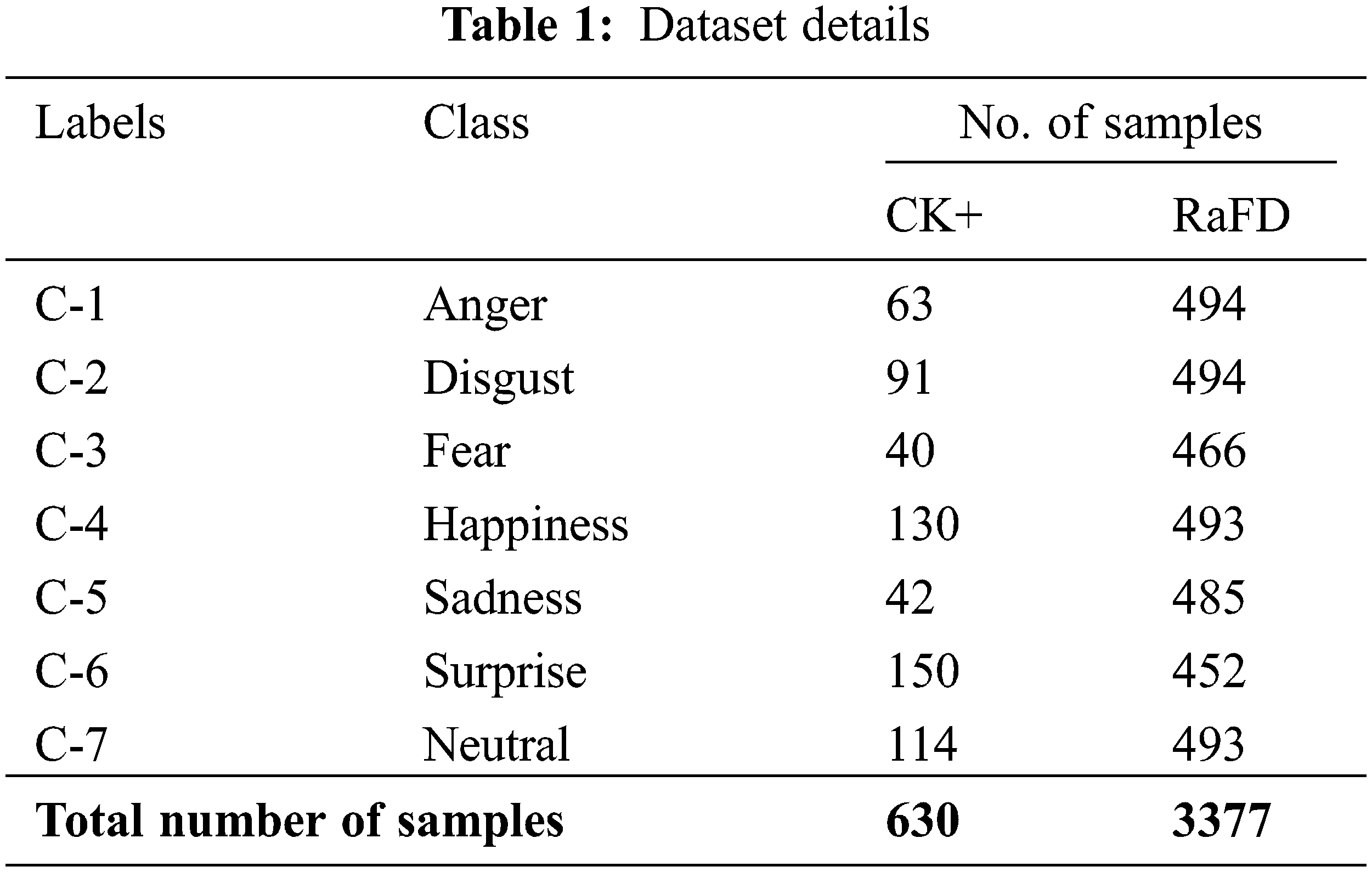
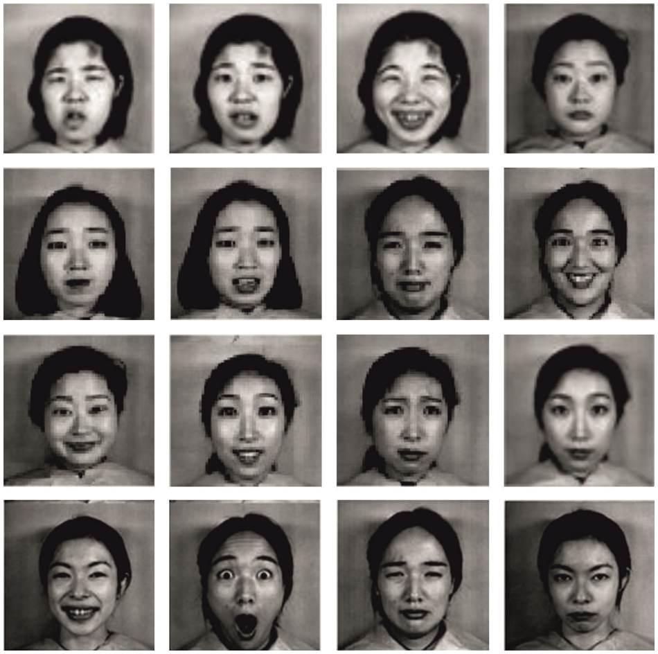
Figure 3: Sample images
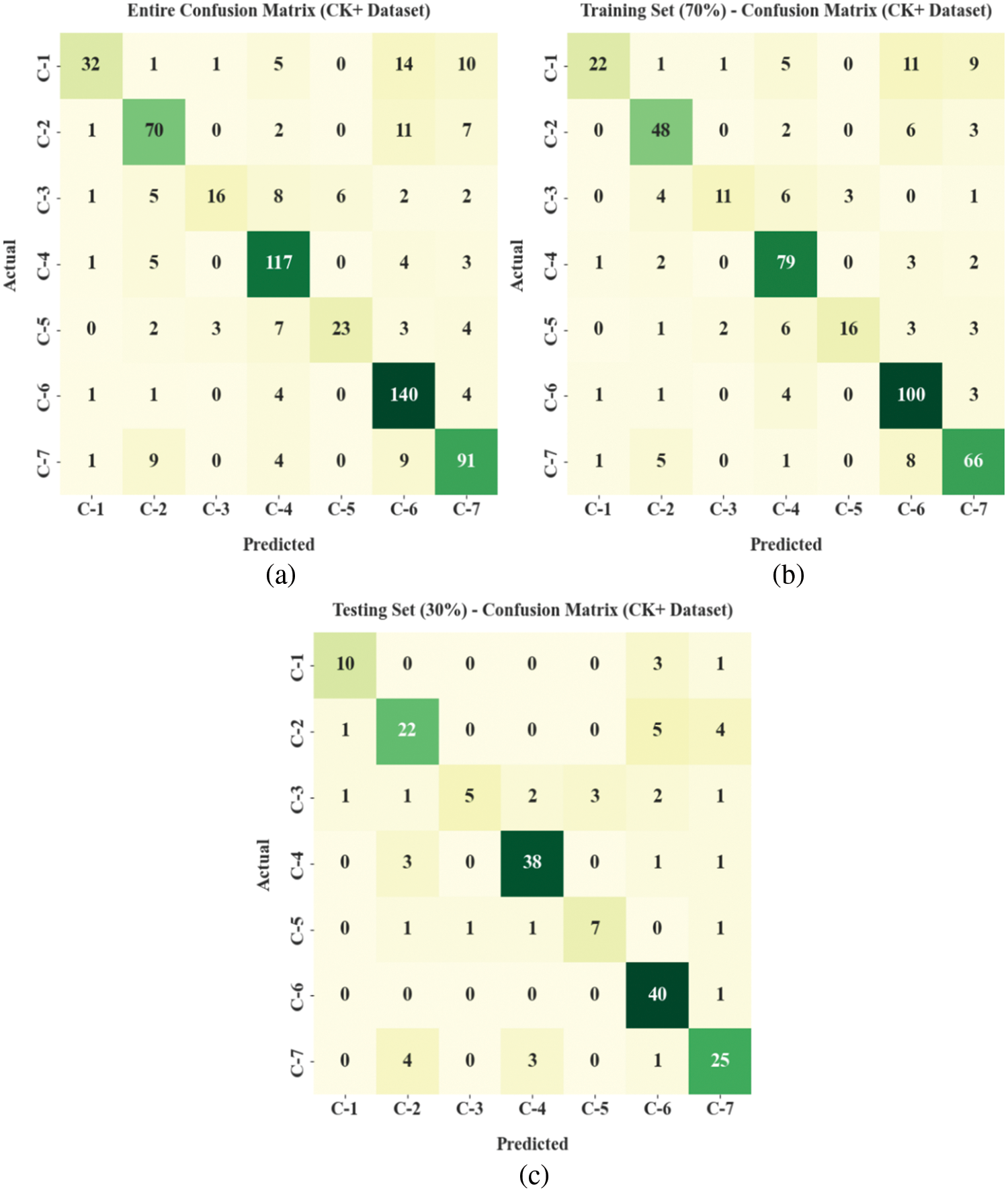
Figure 4: Confusion matrices of EWOISN-FER approach under CK+ dataset (a) Entire dataset, (b) 70% of TR data, and (c) 30% of TS data
Table 2 shows brief FER outcomes of the EWOISN-FER method on the CK+ dataset. The results inferred the effectual FER performance of the EWOISN-FER model over other methods. For example, on the entire dataset, the EWOISN-FER model has offered
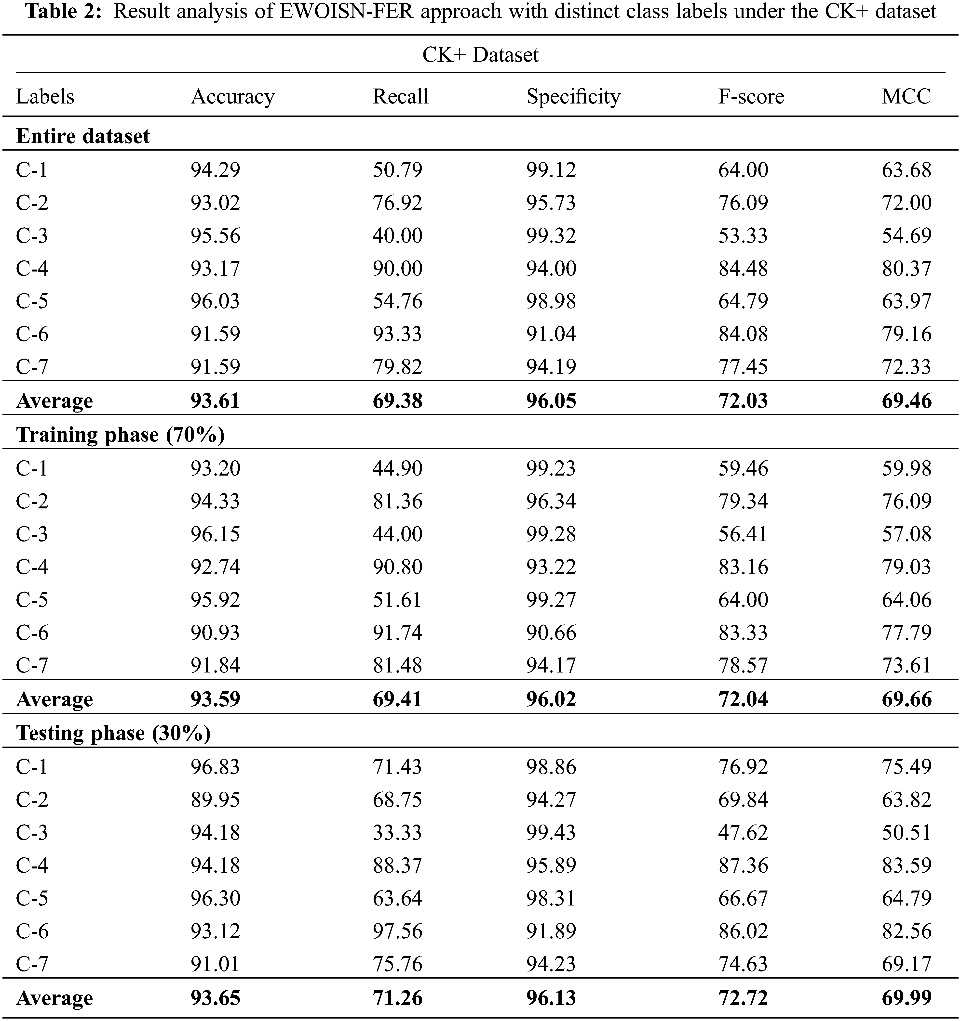
Fig. 5 exhibits the confusion matrices of the EWOISN-FER algorithm on the RaFD dataset. The confusion matrices illustrated that the EWOISN-FER technique could effectually recognise seven different types of facial expressions.
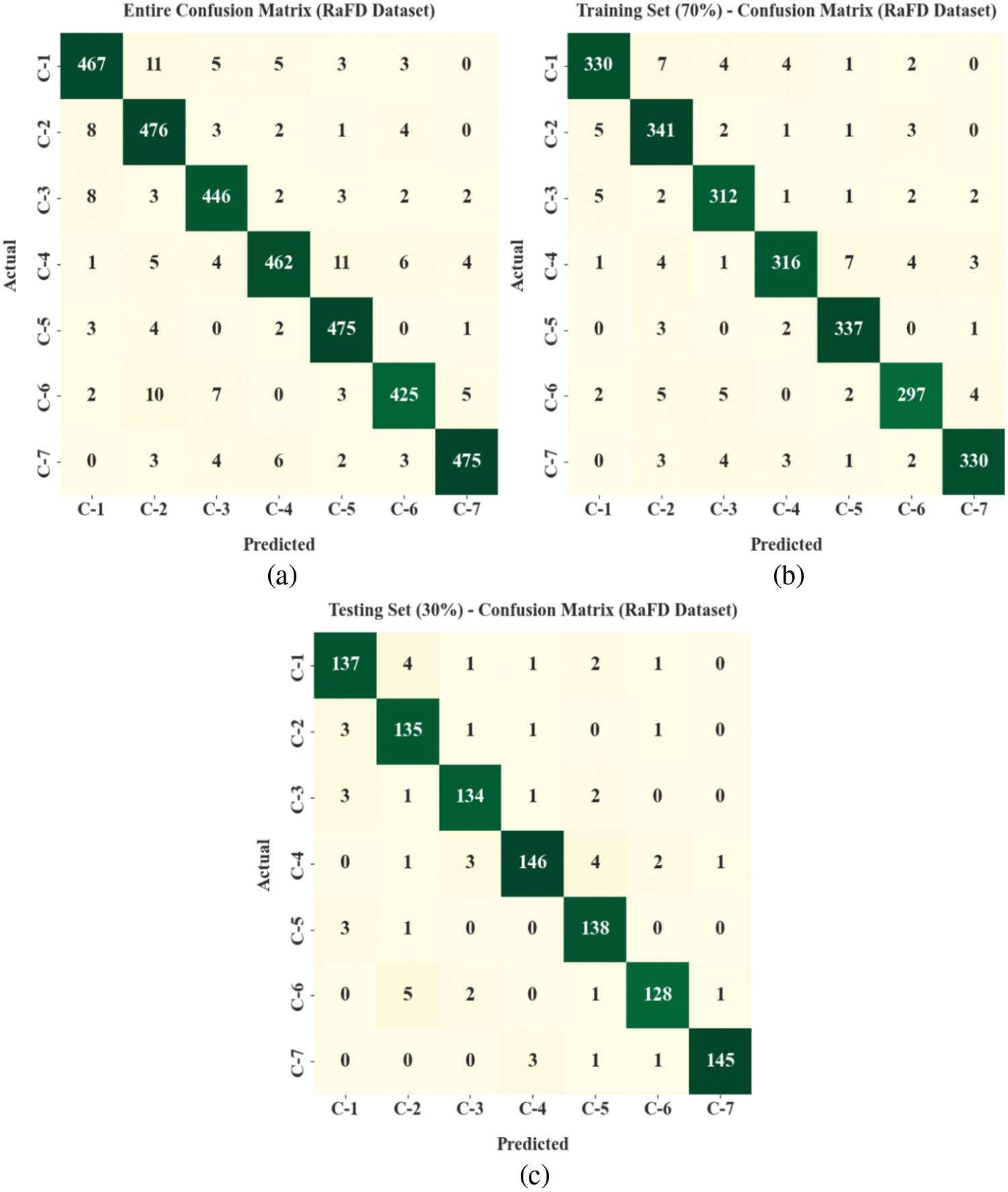
Figure 5: Confusion matrices of EWOISN-FER approach under RaFD dataset (a) Entire dataset, (b) 70% of TR data, and (c) 30% of TS data
Table 3 displays the detailed FER outcomes of the EWOISN-FER technique on the RaFD dataset. The outcomes signify the effectual FER performance of the EWOISN-FER method over other models. For example, on the entire dataset, the EWOISN-FER approach has presented
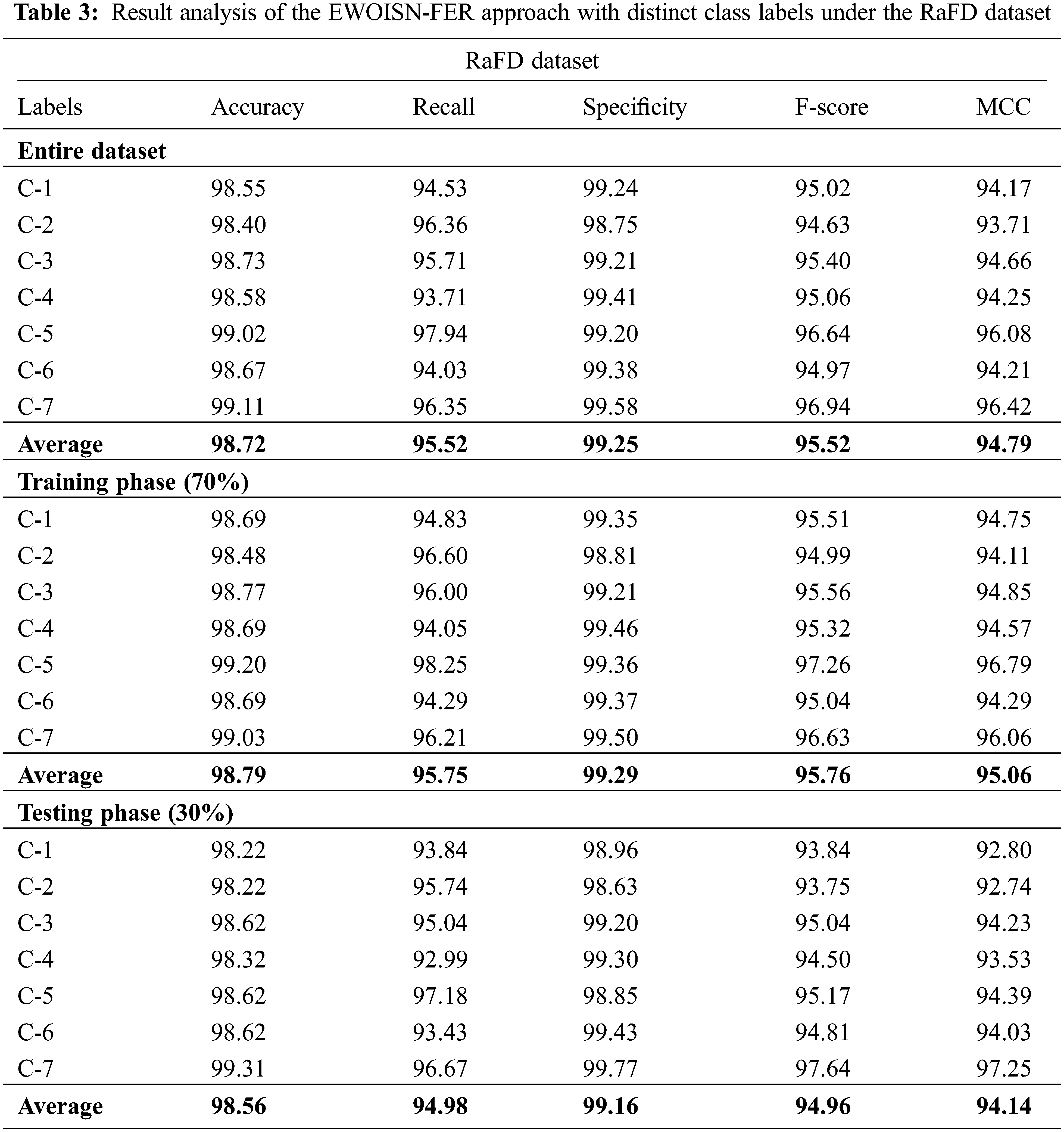
Table 4 provides a detailed
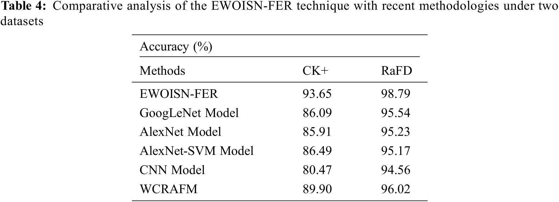
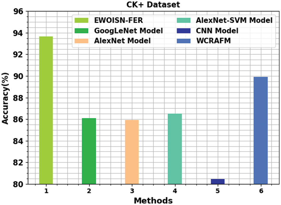
Figure 6:
Fig. 7 establishes a comparative study of the EWOISN-FER algorithm with recent methodologies on the RaFD dataset. The outcomes denote the CNN methodology has exhibited poor results with the least
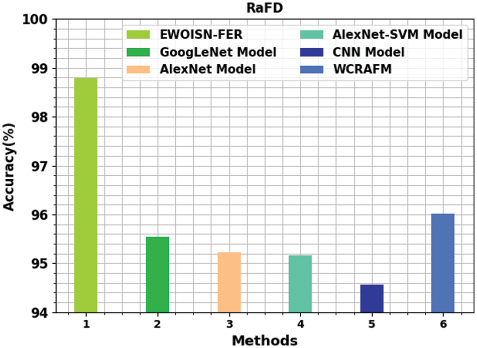
Figure 7:
Therefore, the EWOISN-FER model has exhibited maximum FER performance over other DL models.
In this study, a novel EWOISN-FER approach was projected to recognise and classify facial emotions. The presented EWOISN-FER model employed the CLAHE technique as a pre-processing step. In addition, an improved SqueezeNet model is exploited to derive an optimal set of feature vectors, and the SGB model can execute the hyperparameter tuning process. Lastly, EWO with SAE is employed for the FER process, and the EWO algorithm appropriately chooses the SAE parameters. A wide-ranging experimental analysis is carried out to demonstrate the enhanced performance of the EWOISN-FER technique. The experimental outcomes indicate the supremacy of the presented EWOISN-FER technique. Thus, the EWOISN-FER technique can be exploited for enhanced FER outcomes. In the future, hybrid metaheuristics algorithms can be designed to improve the parameter-tuning process.
Funding Statement: The authors received no specific funding for this study.
Conflicts of Interest: The authors declare that they have no conflicts of interest to report regarding the present study.
References
1. S. Li and W. Deng, “Deep facial expression recognition: A survey,” IEEE Transactions on Affective Computing, vol. 13, no. 3, pp. 1195–1215, 2020. [Google Scholar]
2. A. Agrawal and N. Mittal, “Using CNN for facial expression recognition: A study of the effects of kernel size and number of filters on accuracy,” The Visual Computer, vol. 36, no. 2, pp. 405–412, 2020. [Google Scholar]
3. P. Giannopoulos, I. Perikos and I. Hatzilygeroudis, “Deep learning approaches for facial emotion recognition: A case study on FER-2013,” in Advances in Hybridization of Intelligent Methods, Smart Innovation, Systems and Technologies Book Series, Cham: Springer, vol. 85, pp. 1–16, 2018. [Google Scholar]
4. N. Samadiani, G. Huang, B. Cai, W. Luo, C. H. Chi et al., “A review on automatic facial expression recognition systems assisted by multimodal sensor data,” Sensors, vol. 19, no. 8, pp. 1863, 2019. [Google Scholar]
5. P. W. Kim, “Image super-resolution model using an improved deep learning-based facial expression analysis,” Multimedia Systems, vol. 27, no. 4, pp. 615–625, 2021. [Google Scholar]
6. K. Kottursamy, “A review on finding efficient approach to detect customer emotion analysis using deep learning analysis,” Journal of Trends in Computer Science and Smart Technology, vol. 3, no. 2, pp. 95–113, 2021. [Google Scholar]
7. L. Schoneveld, A. Othmani and H. Abdelkawy, “Leveraging recent advances in deep learning for audio-visual emotion recognition,” Pattern Recognition Letters, vol. 146, pp. 1–7, 2021. [Google Scholar]
8. A. H. Sham, K. Aktas, D. Rizhinashvili, D. Kuklianov, F. Alisinanoglu et al., “Ethical AI in facial expression analysis: Racial bias,” Signal, Image and Video Processing, vol. 146, pp. 1–8, 2022. [Google Scholar]
9. S. Li and Y. Bai, “Deep learning and improved HMM training algorithm and its analysis in facial expression recognition of sports athletes,” Computational Intelligence and Neuroscience, vol. 2022, pp. 1–12, 2022. [Google Scholar]
10. S. Umer, R. K. Rout, C. Pero and M. Nappi, “Facial expression recognition with trade-offs between data augmentation and deep learning features,” Journal of Ambient Intelligence and Humanized Computing, vol. 13, no. 2, pp. 721–735, 2022. [Google Scholar]
11. O. M. Nezami, M. Dras, L. Hamey, D. Richards, S. Wan et al., “Automatic recognition of student engagement using deep learning and facial expression,” in Joint European Conf. on Machine Learning and Knowledge Discovery in Databases, Cham: Springer, vol. 11908, pp. 273–289, 2020. [Google Scholar]
12. G. Bargshady, X. Zhou, R. C. Deo, J. Soar, F. Whittaker et al., “Enhanced deep learning algorithm development to detect pain intensity from facial expression images,” Expert Systems with Applications, vol. 149, pp. 113305, 2020. [Google Scholar]
13. W. M. Alenazy and A. S. Alqahtani, “Gravitational search algorithm based optimized deep learning model with diverse set of features for facial expression recognition,” Journal of Ambient Intelligence and Humanized Computing, vol. 12, no. 2, pp. 1631–1646, 2021. [Google Scholar]
14. J. Liu, Y. Feng and H. Wang, “Facial expression recognition using pose-guided face alignment and discriminative features based on deep learning,” IEEE Access, vol. 9, pp. 69267–69277, 2021. [Google Scholar]
15. S. Minaee, M. Minaei and A. Abdolrashidi, “Deep-emotion: Facial expression recognition using attentional convolutional network,” Sensors, vol. 21, no. 9, pp. 3046, 2021. [Google Scholar]
16. J. H. Kim, B. G. Kim, P. P. Roy and D. M. Jeong, “Efficient facial expression recognition algorithm based on hierarchical deep neural network structure,” IEEE Access, vol. 7, pp. 41273–41285, 2019. [Google Scholar]
17. U. Kuran and E. C. Kuran, “Parameter selection for CLAHE using multi-objective cuckoo search algorithm for image contrast enhancement,” Intelligent Systems with Applications, vol. 12, pp. 200051, 2021. [Google Scholar]
18. H. J. Lee, I. Ullah, W. Wan, Y. Gao and Z. Fang, “Real-time vehicle make and model recognition with the residual SqueezeNet architecture,” Sensors, vol. 19, no. 5, pp. 982, 2019. [Google Scholar]
19. J. H. Friedman, “Stochastic gradient boosting,” Computational Statistics & Data Analysis, vol. 38, no. 4, pp. 367–378, 2002. [Google Scholar]
20. N. Esmaeili, F. E. K. Saraei, A. E. Pirbazari, F. S. Tabatabai-Yazdi, Z. Khodaee et al., “Estimation of 2, 4-dichlorophenol photocatalytic removal using different artificial intelligence approaches,” Chemical Product and Process Modeling, vol. 18, no. 1, pp. 1–17, 2022, https://doi.org/10.1515/cppm-2021-0065. [Google Scholar]
21. K. Zhang, J. Zhang, X. Ma, C. Yao, L. Zhang et al., “History matching of naturally fractured reservoirs using a deep sparse autoencoder,” SPE Journal, vol. 26, no. 4, pp. 1700–1721, 2021. [Google Scholar]
22. S. R. Kanna, K. Sivakumar and N. Lingaraj, “Development of deer hunting linked earthworm optimization algorithm for solving large scale traveling salesman problem,” Knowledge-Based Systems, vol. 227, pp. 107199, 2021. [Google Scholar]
23. P. Lucey, J. F. Cohn, T. Kanade, J. Saragih, Z. Ambadar et al., “The extended cohn-kanade dataset (CK+A complete dataset for action unit and emotion-specified expression,” in IEEE Computer Society Conf. on Computer Vision and Pattern Recognition-Workshops, San Francisco, CA, USA, pp. 94–101, 2010. [Google Scholar]
24. O. Langner, R. Dotsch, G. Bijlstra, D. H. J. Wigboldus, S. T. Hawk et al., “Presentation and validation of the radboud faces database,” Cognition and Emotion, vol. 24, no. 8, pp. 1377–1388, 2010. [Google Scholar]
25. B. F. Wu and C. H. Lin, “Daptive feature mapping for customizing deep learning based facial expression recognition model,” IEEE Access, vol. 6, pp. 12451–12461, 2018. [Google Scholar]
Cite This Article
 Copyright © 2023 The Author(s). Published by Tech Science Press.
This work is licensed under a Creative Commons Attribution 4.0 International License , which permits unrestricted use, distribution, and reproduction in any medium, provided the original work is properly cited.
 Downloads
 Citation Tools