Acoustic Emission Recognition Based on a Three-Streams Neural Network with Attention

1  Introduction

The powerful identification and classification of AE signal of the rotor are very important to the early analysis of rubbing state degree, early diagnosis of mechanical faults, and fault development trend early warning. Many ways have been proposed to extract robust characteristics, which are the properties of the rotor’s rubbing acoustic emission signal. Derived from traditional propagation theory, Modal Acoustic Emission (MAE) technology effectively represents AE signals. It uses multimodal suppression to resolve AE signals into fundamental modal sound waves. And then, it extracts the AE signal’s property parameters. A method called Gaussian mixture model (GMM) which is able to classify rubbing fault, for instance, was proposed by Deng et al. in 2014 and the cepstral coefficient of the AE signal is utilized as an input feature [1]. In addition, some traditional methods are also applied in this field which is about machine learning, such as the Bayesian classifier [2], the support vector machine (SVM) [3], and the K-NN algorithm [4].

The neural network represented by CNN is also used in the field of fault detection [5] with the mushroom growth of deep learning. In 1989, LeCun et al. of New York University (NYU) [6] proposed the CNN, and used it to handle high-dimensional grid data. In the fault diagnosis field, a CNN model combined with the input of AE signal was proposed to detect bearing faults [7] which improves recognition efficiency and level compared with traditional methods. In the same way, CNN can also use to cope with the work of AE. Other methods such as acoustic emission [8–10] and K-means [11] are utilized to improve the performance.

Although CNN has strong processing power in image and other fields, AE signal is essentially a time-dependent signal. In the field of sequential tasks, Long Short-Term Memory (LSTM) neural network, a variation of RNN, plays a crucial role. With the advent of the attention mechanism, initially applied in the field of image processing and achieved excellent results [12], the structure of LSTM-Attention is diffusely applied in the Natural Language Processing (NLP) [13] fields as well as speech processing to obtain the sentence-level embedding [14]. For AE, in this paper, the structure is considered to be equally effective.

Researchers have studied many interesting diagnosis methods of vibration analysis of rolling element bearings. However, the potential of multi-streams neural network has never been tried. Multi-stream neural network is known to be better at feature extraction in areas like facial expression recognition than single-stream neural networks [15]. Fault detection [16]. As a result, in order to accurately identify the AE signal, an improved neural network called TSANN is proposed in this paper. First of all, the AE signal’s time-frequency analysis is performed to determine how frequently AE signals occur over a given period of time. Secondly, three streams of input data are created by calculating the STFT, MFCC, and Tempogram. Then, each stream of the model is used to extract a unique feature representation through CNN-LSTM. To better focus on the most effective features, attention is applied to the output of LSTM. Finally, experiments are used to confirm the availability of the TSANN network, which is proposed in this paper.

2  Main Principle

2.1 Residual Connection Network

Residual connection network was originated from ResNet [17] which is an improvement to traditional CNN models and has become the most popular CNN structure to extract features so far. The original experience shows that the deeper CNN is, the more various extracted features will be. However, more experiments demonstrate that optimization suffers and accuracy falls as a result of gradient disappearance and gradient explosion that deepening the network will bring about. As is shown in Fig. 1, batch normalization will only alleviate this impact to a limited extent, hence the introduction of residual connection. The main idea of residual connection network is that it will directly add the input to the output of current layer so that the shape of tensors must be the same. In the function layer, we adopted the same structure as Fig. 1b.

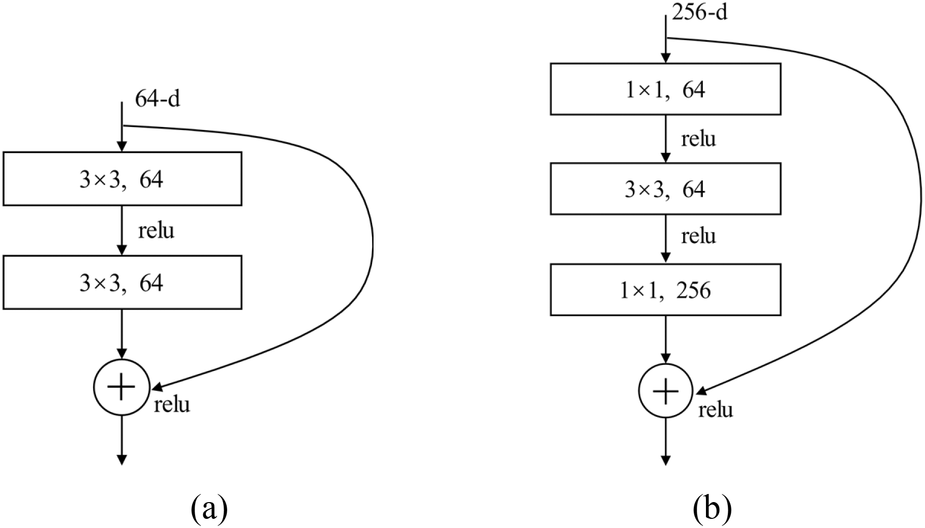
Figure 1: The ResNet Block structure. (a) a ResNet-34 building block. (b) a ResNet-50/101/152 bottleneck building block

2.2 LSTM

A type of time-recurrent neural network called LSTM aims to address the long-term dependence. In our model, LSTM is used to extract time features because there still are acoustic characteristics related to time in AE signal.

2.3 Scaled Dot Product Attention

Scaled dot product attention has gained popularity in tasks involving sequence learning in recent years, which is mainly used to enhance the representation of the current word by introducing context information. The attention structure is shown in Fig. 2 and the final score is calculated as follows:

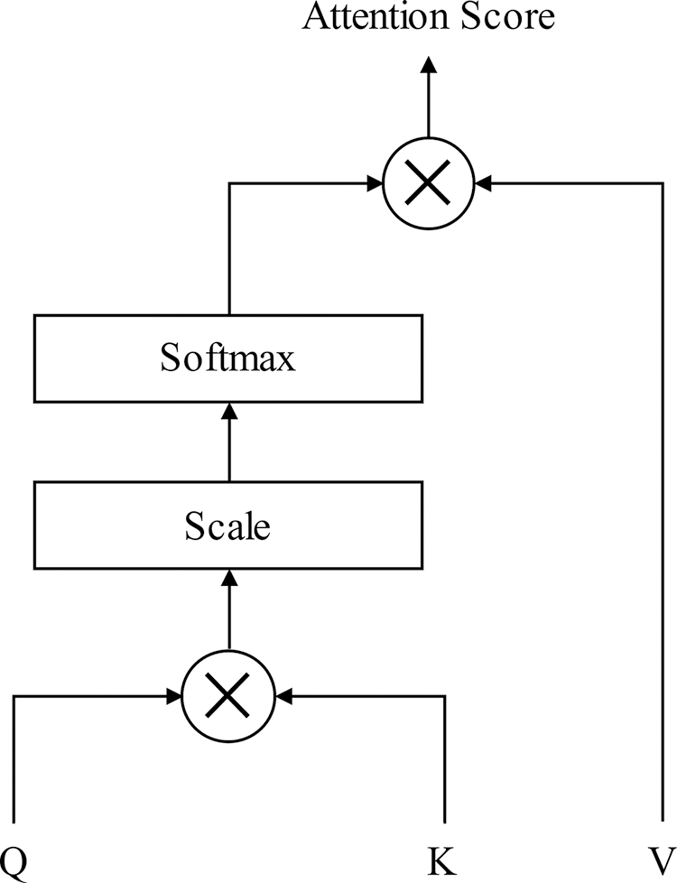
Figure 2: The scaled dot product attention structure

A=QKTd(1)

Score=Softmax(A)∗V(2)

softmax(A)=eA∑j=1NeAj(3)

where Q, K, V is considered to be the same input vectors in each stream with the shape of (N, d), N represents the sequence length of input, and d represents the sequence’s dimension of input.

2.4 Three-Streams Input

Rotating machine rotor AE signal, considered as short-term stationery, is a sort of acoustic signal, just like the natural speech [18]. Therefore, spectral analysis is first performed on AE signal. Fig. 3 presents the spectra of STFT, MFCC, and Tempo of three kinds AE signals respectively, which obviously shows that the three kinds of AE signals exhibit different characteristics. We designed a three-streams input based on the unitary frequency distribution and generally stable of the CNN’s excellent learning classification capacity and the three types of spectrum.

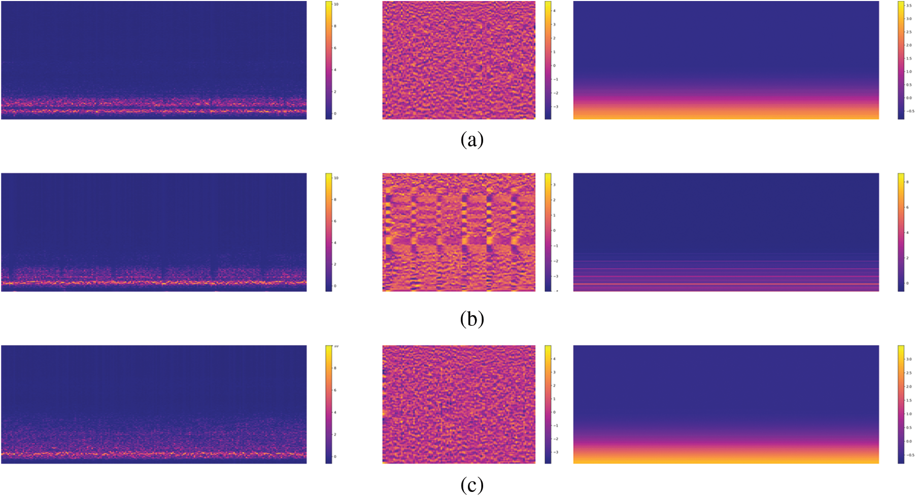
Figure 3: STFT spectra and MFCC of normal, cracking, and rubbing AE signals. (a) Normal. (b) Cracking. (c) Rubbing

STFT. The STFT computes the discrete Fourier transform (DFT) on a short overlapping window to represent signals in the time-frequency domain. Each column in the STFT represents a 512 point FFT of a single signal frame, each frame in it has a duration of 1.024 ms with an overlap rate of 0.5. Since network can only learn the real values, we use the amplitude of STFT which is as known as magnitude instead of raw STFT, and so do other extracted features if necessary.

MFCC. The MFCC takes into account the traits of human hearing by way of mapping linear frequency spectrum to Mel nonlinear frequency spectrum, which converts to the cepstrum and based totally on auditory perception. Each column in MFCC conducts a 2048 points FFT signal’s one frame, and each frame has a continuance of 4.096 ms, and the overlap rate is 0.25.

Tempo. One of the most valuable representations for tempo is named Tempogram, and it has multiple applications such as beat tracking, music structure analysis, music tempo estimation, and music classification. For AE signal, due to the different types of faults, different characteristics may be exhibited during the average rotation cycle. The frame length and overlap of tempogram are in accordance with those of STFT.

As a result, the input is composed of an STFT stream with the shape of 257 × 200 × 1, an MFCC stream with the shape of 128 × 200 × 1, and a Tempo stream with the shape of 512 × 200 × 1.

2.5 TSANN

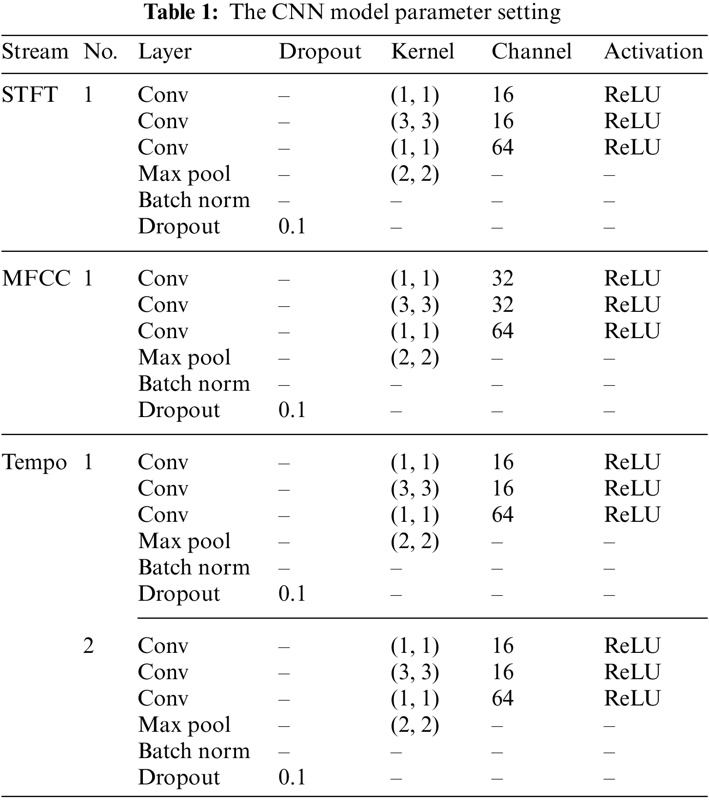
Fig. 4 shows the Basic CNN block based on the ResNet in our mode. The whole CNN structure is one basic block or a superposition of multiple basic blocks. To avoid over-fitting, dropout is adopted in each residual connection block output. Then, LSTM [19] is adopted to obtain time characteristics after CNN. Scaled dot product attention is applied to the output of the LSTM to concentrate on the most useful features. The features of this construction are presented in Table 1.

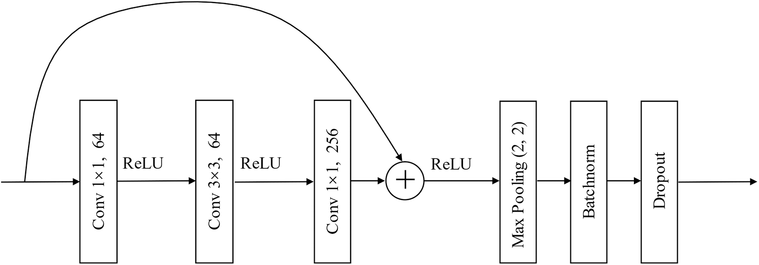
Figure 4: Basic CNN block

The whole TSANN framework is shown in Fig. 5. In the preprocessing stage, the amplitude of STFT, MFCC and Tempogram are extracted by a Python Library named Librosa. Those three features are then input into neural networks with almost the same structures. Outputs on behalf of the highest own representation of each stream are concatenated into a linear layer. As a result, the final output is obtained by a linear layer with softmax activation.

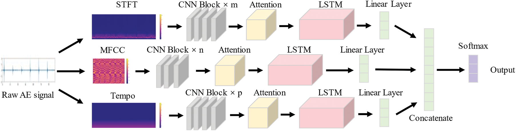
Figure 5: The overall framework

3  Experiments

3.1 Database

We use a database gathered by our laboratory research group during the past years in this paper, which includes rotor cracks, normal signals, and rotor rubbing AE signals composed of the AE signals of rotating machinery to be the AE signal database. In general, the AE signals of the database are at three different rotational speeds, that are 800, 700, and 600 rad/s.

The concrete details of the AE database are shown in Table 2. All of the sampling rates utilized are 500 kHz, and each piece of data sampling time lasts 102.294 ms. In the case of 600 rad/s rotation speed, each AE discrete signal's whole point length is 51147, and continually collects around 9.8 rotor cycles. Fig. 6 depicts the time domain audio waves of the three signals. To compare the differences objectively, the scale on Y-axis is limited in (−2, 2).

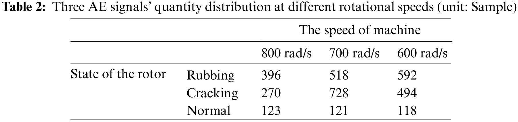
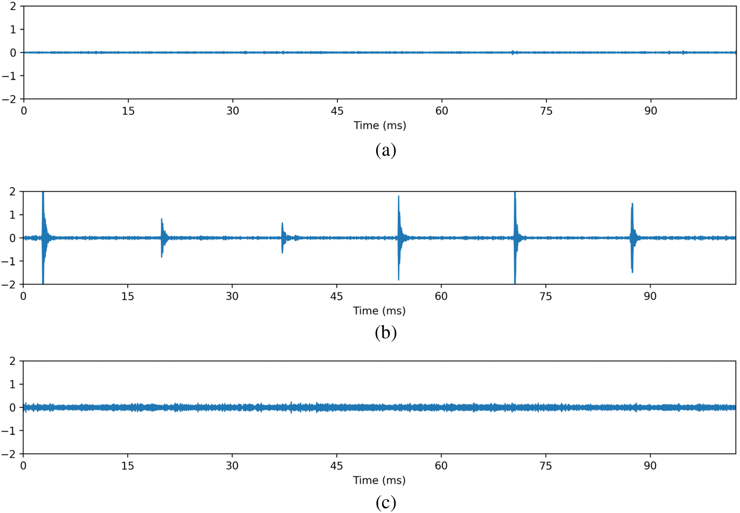
Figure 6: The database samples. (a) Normal. (b) Cracking. (c) Rubbing

3.2 Experiment Setup

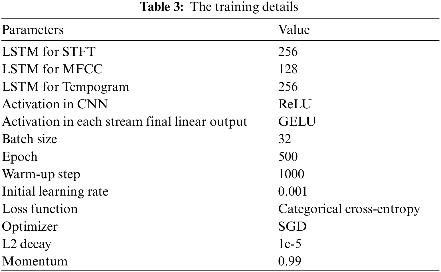
The main experiment uses the AE signal, which has a rotation speed of 600 rad/s. We also used the 700 and 800 rad/s rotation speed of AE signal as the reference experiment. And we used the Hanning window to frame the discrete AE signal, and the frame length choice is mostly determined by the FFT point representation validity. We eventually take the 512 points FFT after carrying out experiments on the 2048 points, 1024v points, 512 points, and 256 points FFTs respectively to construct and train the network well in this experiment, the deep learning framework in PyTorch is used. And the rate of the test set to the training set is 14. As for the activation, ReLU [20], Leaky ReLU [21], and GELU [22] were adopted respectively, and ReLU was taken in the end. SGD optimization algorithm was performed for training. Noam scheme learning rate was adopted which is defined as Eq. (4), where n is current iteration step and w represents warm up steps. Table 3 shows more details of the training section.

learning_rate=(init_lr⋅w)−0.5⋅min(n−0.5,n⋅w−1.5)(4)

3.3 Result Analysis

3.3.1 Recognition Result

The recognition accuracy is measured by UAR (Unweighted Average Recall). Fig. 7 shows the comparison among the network if LSTM is introduced or not. It can be figured out that there is an obvious increase for MFCC, while only slight improvements for the other features, which indicates that MFCC contains more characteristics in time dimension. As for the tempogram, the reason for such a slight increase is that tempo is considered as a measure of the speed of music which may be less obvious in AE signals, but it still works to some extent.

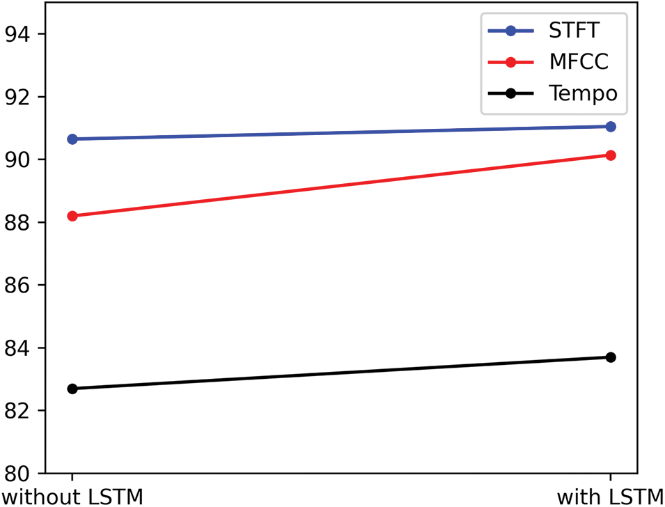
Figure 7: The contrast after and before introducing LSTM module

The confusion matrices of different models are presented in Fig. 8 of which the number in figures represents the number of samples. Fig. 9 reflects the average recognition performance between single-stream CNN (abbreviated as SS) and TSANN. Compared to SS, the proposed model performs better. The accuracy of Normal and Rubbing are the key to restrict the overall recognition performance for both SS and TSANN. By combining three SS models, the classification error rate for Normal was reduced by half, and it has been reduced to varying degrees for other categories.

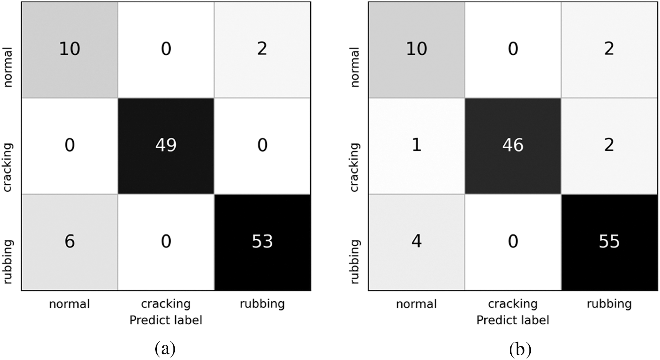
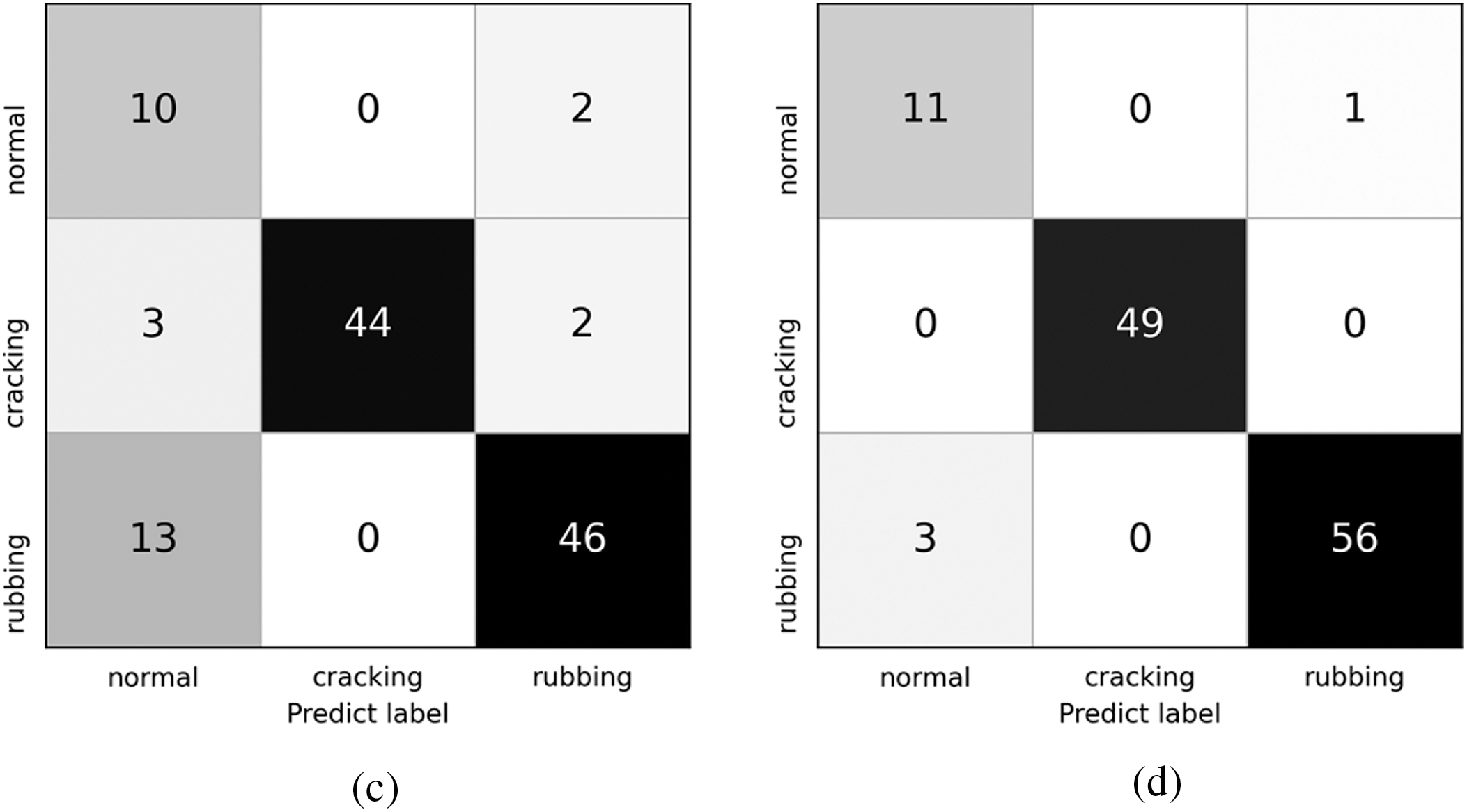
Figure 8: The confusion matrices of the single-stream CNNs and TSANN. (a) STFT. (b) MFCC. (c) Tempogram. (d) Three-streams CNN

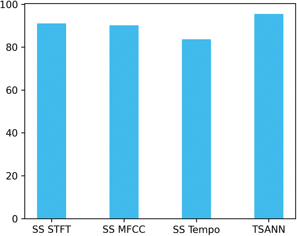
Figure 9: Different networks’ UAR

3.3.2 Model Comparison Experiment

The traditional ways to identify AE signals are compared to further discover the capability of the model. Different classifiers of AE signal classification capability is shown in Table 4, and Fig. 10 also shows the results.

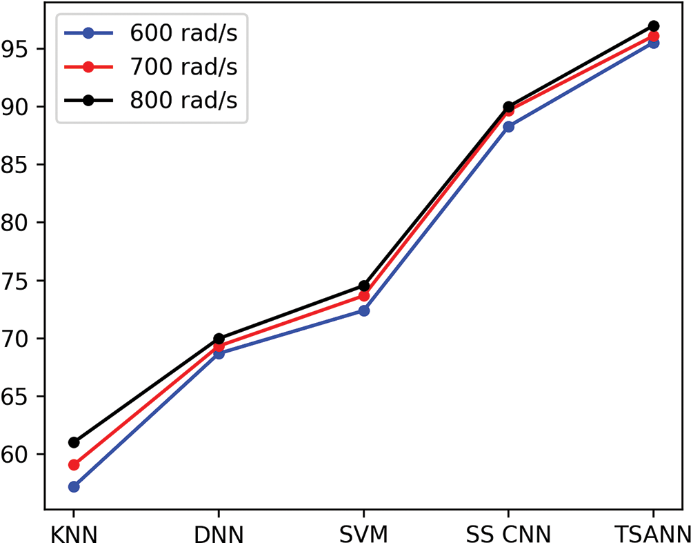
Figure 10: UAR of different models at three speeds

The table shows that the proposed way’s recognition accuracy performance is the best for all Rubbing, Cracking, and Normal, AE signals. The whole average recognition rate is more than 20% higher than SVM, which has the best capability among the traditional classification methods, reaching 72.40% on average. On Rubbing AE signal, the classifier KNN has a poor recognition impact, with a recognition rate of 57.23% overall. Compared with DNN and single-stream CNN, which are also neural networks, since there are three-streams inputs in TSANN, raw AE signals can effectively capture more features, leading to the highest UAR of 95.53%. Furthermore, the shallow CNN which only has 1 or 2 CNN blocks is better suited for the training of small datasets compared with the deep CNN.

3.4 Speed Comparison Experiment

Ultimately, we compare AE signals at different speeds to explore the influence of machine speed on AE signals recognition performance. Experimental results reveal that TSANN gets the best performance under conditions of different speeds. In comparison with traditional methods such as SVM and KNN, methods with CNN make an incredible improvement. Besides, UAR of each model is relatively stable at different speeds, although the higher speeds may account for higher accuracy to a small extent, indicating that more sufficient loads for triggering AE signal are provided with the increasement of speed and thus promoting the classification of AE signals within a reasonable range.

4  Conclusion

In this paper, a novel three-streams neural network called TSANN is proposed and we uses it to detect rotor rubbing AE faults. The model takes into consideration the peculiarities of STFT, MFCC, and Tempogram, and combines them into a three-streams input to feed into different CNN-Attention-LSTM structures. Residual connection is adopted in CNN to avoid the problems of gradient disappearance and gradient explosion. Scaled dot product attention is used for obtaining more important feature representation. LSTM performs a slightly better performance in dealing with the time information contained in the audio signals. We conduct multiple experiments to verify the capability of TSANN. In comparison with other traditional classification ways, the proposed CNN structure achieves a relatively high recognition accuracy. In addition, the recognition error rate of TSANN decreased in varying degrees compared with single-stream model.

Acknowledgement: The authors would like to thank the College of Information and Engineering, Xuzhou University of Technology.

Funding Statement: The authors received no specific funding for this study.

Conflicts of Interest: The authors declare that they have no conflicts of interest to report regarding the present study.

References

1. A. Deng, H. Cao, H. Tong, L. Zhao, K. Qin et al., “Recognition of acoustic emission signal based on the algorithms of tdnn and gmm,” Applied Mathematics & Information Sciences, vol. 8, no. 2, pp. 907, 2014. [Google Scholar]
2. P. Baraldi, L. Podofillini, L. Mkrtchyan, E. Zio and V. Dang, “Comparing the treatment of uncertainty in bayesian networks and fuzzy expert systems used for a human reliability analysis application,” Reliability Engineering & System Safety, vol. 138, no. 2–3, pp. 176–193, 2015. [Google Scholar]
3. V. Vapnik, The Nature of Statistical Learning Theory. London SW1P 1WG, UK: Springer science & business media, Taylor and Francis Press, 1999. [Google Scholar]
4. D. Wang, “K-nearest neighbors based methods for identification of different gear crack levels under different motor speeds and loads: Revisited,” Mechanical Systems and Signal Processing, vol. 70, no. 1, pp. 201–208, 2016. [Google Scholar]
5. Y. Lei, F. Jia, J. Lin, S. Xing and S. X. Ding, “An intelligent fault diagnosis method using unsupervised feature learning towards mechanical big data,” IEEE Transactions on Industrial Electronics, vol. 63, no. 5, pp. 3137–3147, 2016. [Google Scholar]
6. Y. LeCun, L. Bottou, Y. Bengio and P. Haffner, “Gradient-based learning applied to document recognition,” Proceedings of the IEEE, vol. 86, no. 11, pp. 2278–2324, 1998. [Google Scholar]
7. A. Prosvirin, J. Kim and J. M. Kim, “Bearing fault diagnosis based on convolutional neural networks with kurtogram representation of acoustic emission signals,” in Advances in Computer Science and Ubiquitous Computing, New York, NY, United States: Springer, pp. 21–26, 2017. [Google Scholar]
8. L. Jing, Y. Yong, H. Ge, Z. Li and R. Guo, “Coal rock condition detection model using acoustic emission and light gradient boosting machine,” Computers, Materials & Continua, vol. 63, no. 1, pp. 151–161, 2020. [Google Scholar]
9. W. Wang, W. Liu, J. Liu and M. Zhang, “Acoustic emission recognition based on a two-streams convolutional neural network,” Computers, Materials & Continua, vol. 64, no. 1, pp. 515–525, 2020. [Google Scholar]
10. L. Zhao, X. Chen, J. Cheng, L. Yu, C. Lv et al., “New three-dimensional assessment model and optimization of acoustic positioning system,” Computers, Materials & Continua, vol. 64, no. 2, pp. 1005–1023, 2020. [Google Scholar]
11. A. A. Ahmed and B. Akay, “A survey and systematic categorization of parallel k-means and fuzzy-c-means algorithms,” Computer Systems Science and Engineering, vol. 34, no. 5, pp. 259–281, 2019. [Google Scholar]
12. F. Wang, M. Jiang, C. Qian, S. Yang, C. Li et al., “Residual attention network for image classification,” in Proc. of the IEEE Conf. on Computer Vision and Pattern Recognition, Honolulu, HI, pp. 3156–3164, 2017. [Google Scholar]
13. D. Bahdanau, K. Cho and Y. Bengio, “Neural machine translation by jointly learning to align and translate,” arXiv preprint, arXiv:1409.0473, 2014. [Google Scholar]
14. Z. Lin, M. Feng, C. N. D. Santos, M. Yu, B. Xiang et al., “A structured self-attentive sentence embedding,” arXiv preprint, arXiv:1703.03130, 2017. [Google Scholar]
15. H. Q. Khor, J. See, R. C. W. Phan and W. Lin, “Enriched long-term recurrent convolutional network for facial micro-expression recognition,” in 13th IEEE Int. Conf. on Automatic Face & Gesture Recognition, Xi'an, China, pp. 667–674, 2018. [Google Scholar]
16. X. Li, J. Li, Y. Qu and D. He, “Gear pitting fault diagnosis using integrated cnn and gru network with both vibration and acoustic emission signals,” Applied Sciences, vol. 9, no. 4, pp. 768–768, 2019. [Google Scholar]
17. K. He, X. Zhang, S. Ren and J. Sun, “Deep residual learning for image recognition,” in Proc. of the IEEE Conf. on Computer Vision and Pattern Recognition, Las Vegas, NV, USA, pp. 770–778, 2016. [Google Scholar]
18. P. Kundu, N. K. Kishore and A. K. Sinha, “A non-iterative partial discharge source location method for transformers employing acoustic emission techniques,” Applied Acoustics, vol. 70, no. 11–12, pp. 1378–1383, 2009. [Google Scholar]
19. S. Hochreiter and J. Schmidhuber, “Long short-term memory,” Neural Computation, vol. 9, no. 8, pp. 1735–1780, 1997. [Google Scholar] [PubMed]
20. V. Nair and G. E. Hinton, “Rectified linear units improve restricted boltzmann machines,” in Proc. of the 27th Int. Conf. on Machine Learning, Haifa, Israel, pp. 807–814, 2010. [Google Scholar]
21. B. Xu, N. Wang, T. Chen and M. Li, “Empirical evaluation of rectified activations in convolutional network,” arXiv preprint arXiv:1505.00853, 2015. [Google Scholar]
22. D. Hendrycks and K. Gimpel, “Gaussian error linear units (gelus),” arXiv preprint arXiv:1606.08415, 2016. [Google Scholar]
Cite This Article
Copyright © 2023 The Author(s). Published by Tech Science Press.
This work is licensed under a Creative Commons Attribution 4.0 International License , which permits unrestricted use, distribution, and reproduction in any medium, provided the original work is properly cited.
Downloads
Citation Tools