SMOGN, MFO, and XGBoost Based Excitation Current Prediction Model for Synchronous Machine

1  Introduction

In modern industry, some devices are operated according to the electromagnetic induction theory, such as motors, transformers, etc. In this regard, the motor relies upon a critical performance indicator and it is the power factor. The power factor is the ratio between the active power and the reactive power. The active power transforms the electric energy into mechanical energy and luminous energy, etc., and it is the power that can reflect the operational capability level of the component. In comparison, reactive power is the electric power that maintains the exchanging action between the magnetic field and the electric field in the AC circuit. Still, it does supply any power to the external devices. Without reactive power, it would be impossible for the motor and the transformer to operate. The reactive power compensation will be required if the synchronous motor should maintain high power factor operation under varied load ratings. In [1,2], the fuzzy logic control synchronous motor is used for achieving the reactive power compensation. It proves that the system will be allowed to input the required reactive power according to varied load ratings through the Fuzzy logic control in a quicker way. The reactive power compensation can be realized through other methods [3], like the excitation current adjusting because the excitation current can directly change the reactive power of the synchronous motor, for the motor to operate according to the required power factor. In terms of this, the algorithm model proposed in this article is the method that can accurately predict the desired excitation current, so that the synchronous motor can provide the required excitation current according to varying load ratings to operate within the expected power factor range to achieve higher motor performance.

The first motors were built in the 19th century. Motors have now become indispensable to modern life. They are used everywhere and can be of several different types, the most commonly used being Direct Current (DC) motors, single-phase, and three-phase Alternating Current (AC) motors. DC motors can be divided into magnetic coils or permanent magnets, and the basic working principle of a magnetic coil motor is that when certain current flows through the coil between the magnetic poles inside the motor, there will generate a magnetic field generated according to Fleming’s left-hand rule, thereby pushing the coil to rotate continuously. On the other hand, permanent magnets can use either in DC or AC motors, where the DC one is called Brush-less DC Motor (BLDC) and the AC one is called Permanent Magnet Synchronous Motor (PMSM). The significant difference between BLDC and PMSM is the former is driven by square waves while the latter is driven by sine waves. However, both of them use permanent magnets as rotors. There is no coil in the rotor, and the current is not transmitted by carbon brushes but generated by electromagnetic induction to push the rotor. Due to no carbon brushes, DC motors have distinct advantages concerning maintenance.

AC motors can be divided into synchronous motors and induction motors. When the rotational speed of the rotor is slower than the speed of the magnetic field, then it is an induction motor. In this study, three-phase synchronous motors were used where the speed is constant and determined by the frequency of the AC power supply. The rotational speed of a synchronous motor is dependent on the frequency of the power supply, not the voltage. Furthermore, the rotational speed will not be affected by changes in load as long as they are less than the maximum torque of the motor. Synchronous motors are not self-starting and in this study, the shaft of the synchronous motor was coupled with the shaft of another motor to drive it up to close to its synchronous speed because no other self-starting mode was available. However, the most common way of starting a synchronous motor is by running them as induction motors until the rotation speed is close to synchronization. This is usually achieved using damper windings. When the rotor reaches synchronization speed, the damper winding goes out of the circuit because the rotating magnetic field is equal, and the current will be zero. Induction operation in powerful 3-phase motors is a high current, and for starting the motor windings are connected in a star configuration. This is switched over to delta for synchronous operation.

Reactive power compensation [4,5] is indispensably applied in industrial equipment. It is not only connected with the value of the power factor but is also proportional to the voltage value. Therefore, reactive power compensation can enhance the quality of the power supply, improve the power factor and reduce the loss of active power. It also reduces costs and stabilizes the operation of the equipment. The power factor of a synchronous motor operating under a fixed load at synchronous speed can be adjusted by changing the excitation current of the magnetic field. This correction of the power factor can stabilize the voltage and the operation of the motor. This makes synchronous motors very useful for pumps, compressors, and many kinds of machinery because of their constant speed.

Because the parameters indicated in the mathematical expression of the synchronous motor are not connected as far as the linearity is concerned, acquiring these parameters through mathematical formulas will require a massive amount of computation. Despite some scholars proposing the Kalman filter-based conventional prediction method [6,7] during the past years, the “Al-based” algorithm has been now regarded as the mainstream research method such as Artificial Neural Networks [8], k-nearest neighbor (k-NN) [9] and Genetic Algorithm (GA) [10]. From the result of [9], the Intuitive k-NN Estimator (IKE), an improved version of k-NN, has a lower error rate of 4%–8% when compared with k-NN and ANN. Since the vigorous progress that has been seen in the development of AI algorithms in recent years, a more suitable algorithm can be applied to the excitation current prediction. Therefore, the method above is referenced by using the optimizer to execute the optimization of the model to acquire a much better result. The optimizer has been frequently applied in motor control or used with other types of controllers. Take [11] for example, the MFO is employed to optimize the parameters of the auto disturbance rejection controller, whereas in [12], the MFO is used with the Fuzzy logic control, for applying the power factor to adjust the power factor of the brushless DC motor. In terms of this, the Genetic Algorithm (GA) and the Particle Swarm Optimization (PSO) are the optimizers that are frequently seen and exhibit satisfactory effects. Further in the research explained in [13–15], the PSO and GA are used in the research to optimize XGBoost (XGB) and Random Forest models by which, the superior result is obtained when compared to the basic model.

This research contributes to finding a model that will be more suitable for predicting the excitation current. All of the basic models will be trained so that the best one can be selected for joining the SMOGN, to deal with the scenario that is provided with fewer data or subjected to unbalanced status to produce uniformly distributed data. The experiment result proves that it can enhance prediction accuracy. After being upgraded, additional optimizers will be added to find out the optimal parameters for the basic models. The result indicated that the prediction result obtained by combining the basic model with the SMOGN and the optimizer model is superior to all previous models, and MFO has the best learning curve and prediction results among all optimizers. On this basis, picking the best model for this dataset and improving the prediction accuracy is the biggest contribution of this study.

Next, this research will explain the data source and its distribution status in Chapter 2. In Chapter 3, this research will introduce the architectural training diagram and the operation theory of the basic model, SMOGN and optimizer models. In Chapter 4, this research will show the model prediction result diagram as well as explain the following three kinds of evaluation indicators, i.e., MAE, RMSE, and R2Score. Finally, make a table and draw a learning curve to compare the accuracy and learning speed of these optimizers. In Chapter 5, the conclusions are made showing that the SMOGN-MFO-XGB presents the most accurate prediction result among all models; to this extent, it allows the motor to operate at appropriate power factor under varied load ratings to reduce the energy loss while enhancing the value of the production line. Finally, the Appendix will explain the architectural diagram and the theory of the seven kinds of basic models in a detailed manner.

2  Synchronous Motor Signals

Five synchronous motor parameters [16] used in this study are shown in Fig. 1, Load Current (Iy), Power factor (PF), Power factor error (e), changing the excitation current of a synchronous machine (dIf), and excitation current of a synchronous machine (If), wherein the load current is a control variable and the power factor is an independent variable. First fix the load current was fixed at three and the power factor was adjusted from 0.66 to 1 with increments of 0.2, when the power factor rises to 1, adjust the load current to increase by 0.1. Then these steps will repeat until the load current increases to 4.6, while the power factor increments were kept to 0.2 until 0.84 and continued to increase from 0.87 to 0.99. The load current was raised from 4.7 to 6 by adjusting the power factor from 0.65 to 0.99 with increments of 0.2. The power factor error was therefore one minus the power factor. In this article, the Iy, PF, and e will be used as the model input, with If used as the output data. As indicated in the figure, If and dIf show very close trends; thus, pretty high correlation, and dIf is the variation of If and so, and dIf is precluded from the training model. Further, e is the value acquired from 1-PF. The power factor [17] is the ratio of active power to apparent power, also interpreted as the ratio of obtained power to actual dissipated power, it is a non-dimensional value between 0 and 1, see Eq. (1) below.

Figure 1: Distribution of data and various parameters in a synchronous motor

PF=|P||S|=cosφ(1)

wherein P is the active power, S is the apparent power, and cosφ is the cosine of the phase difference between voltage and current. Active power, also known as average power, is the average value of instantaneous power made in a period. Apparent power is the product of the effective values of voltage and current in the AC power supply or the combined amount of active power and reactive power. Reactive power reflects the energy exchange between the magnetic field and the electric field. In the circuit, there is no energy consumption by external work. When the current phase lags behind the voltage phase, P is less than S, the so-called power factor lag. However, when the current leads the voltage, this is the power factor leading. The closer the corrected power factor of the power supply used by the motor is to 1, the lower the apparent power, the more stable the voltage, the higher the efficiency, and the lower the cost.

The data above was acquired through the experimental devices indicated in Fig. 2, in which cosφ represents the power factor. Because the synchronous motor cannot move by itself, so the AC voltage is supplied to another motor for the latter to drive the synchronous motor. Soon as the revolution is nearing the synchronized speed, the motor starts inputting the AC voltage to achieve the synchronized operation. Then, the supplying motor will be separated from the synchronous motor. During the synchronized process, the excitation current passes through the series connection point, then it will adjust to the minimal “rheostat”; at this time, the load current and voltage will maintain the fixed value. Next, adjust the excitation current from low to high or from high to low. Soon as the excitation current increases, the power factor of the motor will increase, becoming the “leading power factor”. As a next step, adjust the load current from 3 to 6, with 0.1 increments added each time. Finally, repeat the aforesaid action for testing the experiment result obtained from varied load current ratings and then create the dataset required for the in/out parameters. In this way, This makes the load current and the power factor in many data the input to predict the excitation current. Based on the result thus obtained, the excitation current will regulate for the motor to achieve optimal operating efficiency with the power factor ranging within a specific scope.

Figure 2: Test device for input and output data [9]

3  The Proposed Method

Although 558 pieces of data are not very much, preprocessing is still necessary to reduce the differences between them to improve accuracy before introducing the prediction model. First, the data was normalized [18] to offset and scale them to a number between 0 and 1. This is a standard procedure during data preprocessing so that any significant fluctuations among data are reduced to avoid poor accuracy caused by predicted value errors. The normalization equation is as follows:

xnormalize=x−xminxmax−xmin∈[0,1](2)

wherein xnormalize is the normalized value, xmax and xmin are the maximum and minimum values of the data respectively, and x is the original value [19]. In this study, the MinMaxScaler included in the Scikit-learn package was used to control the scaling interval, after which the “fit transform” function is applied to carry out scaling.

To prevent only specific data from being qualified for obtaining better-predicted results being chosen by the model, the k-fold cross-validation method [20] as shown in Fig. 3 is used for the cross-validation of input data. This was done to avoid selecting specific data by the model and to ensure unbiased prediction. Data was divided into validation and training groups to improve the accountability of model training. The original 558 data were divided into k equal parts. In this study, set k=10 to the extent that it will be roughly divided into ten equal portions with some of them higher or lower but will not affect the exactness of the cross-verification. Take one equal part from these ten equal parts for testing and leave the remaining nine equal parts for training. As each equal part has been taken for testing, there are ten predicted results generated, and a final predicted result will be obtained in a later process either by averaging above mentioned ten results or summarizing them in other ways. In this study, training and validation were done with several different algorithms: MLP, Dense Convolutional Network (DenseNet), Adaptive Boosting (Adaboost), Decision Tree (DT), Random Forest (RF), Support Vector Regression (SVR), and XGB for training. Ultimately, different algorithms are compared by MAE, RMSE, and R2Score to check individual performance.

Figure 3: Schematic diagram of k-fold cross-validation

Artificial neural networks [21] are models that simulate a biological nervous system to reflect the behavior of the human brain. In such models, multiple neurons in layers are connected to neurons in other layers, and the output values are weighted during processing, the performance of the neural network is affected by the settings of intermediate parameters. The machine learning [22] model and its introduction of seven algorithms, including Adaboost, MLP, DenseNet, DT, RF, SVR, and XGB will be introduced in the appendix. Applied the seven algorithms mentioned above to the model described in Fig. 4 to complete the basic training. First, the datasets were read and normalized. Then k-fold cross-validation was normalized, and they were then divided into training data and testing data. The training data is input into all the different models for training, and the testing data is used to obtain the prediction results. Finally, the results are summarized and the accuracy of the different models is compared.

Figure 4: Architecture diagram of basic model training

SMOGN was then used to select the best of these models for optimization. The SMOGN [23] algorithm, mainly deals with fewer data within data imbalance domains to generate well-distributed data. First, a decision is made about which dimension is to be adjusted. The data distribution is then generated according to a box plot to obtain specific control points. Next, the root of the control points is introduced into a Hermite Interpolating Polynomial to define a correlation function with a value range of 0–1; data close to 1 is considered to be over-sampling, and data close to 0 is under-sampling. Then the k-NN method is used: when the distance of a data point from all surrounding neighbors is less than a specific value, interpolation is applied to generate new data. When this distance is more significant than a specific value, it is considered to be a disturbance, and the Gaussian Noise strategy is applied to generate new data.

Several iterations of SMOGN and different optimizers are then applied to the best model found to find the optimal parameters. This study will use the following four optimizer algorithms.

PSO [24,25] is a heuristic algorithm that simulates the feeding and predation behavior of a flock of birds. Each particle acts like a bird and defines individual fitness by the fitness function, thereby getting the best position for the particle itself and the swarm. Later, it will adjust to move according to its own experience and that of the swarm. The equations for the determination of the swarming speed and position of the particles are shown below.

Vi(t+1)=w×Vi(t)+c1×r1×(pi(t)−xi(t))+c2×r2×(pg(t)−xi(t))(3)

xi(t+1)=xi(t)+Vi(t+1)(4)

wherein w is the weight, c1 and c2 are acceleration constants, r1 and r2 are random values within the range [0, 1], Vi(t+1) is the vector value of the velocity at time t + 1, pi(t) is the best position found by the ith particle so far (also called pbest), xi(t) is the current position of the particle, pg(t) is the best position found by the swarm so far (also called gbest); it will calculate the new particle position xi(t+1) using the above equation based on the new velocity Vi(t+1), the flowchart is shown in Fig. 5.

Figure 5: PSO flowchart

The Grey Wolf Optimizer (GWO) [26–28] simulates the daily routine of a wolf pack. The overall architecture of this optimization consists of stratifying, rounding up, and hunting. Stratifying involves the mapping of the best three groups of the overall pack into α,β,δ and leaves the rest as ω. Then, α,β,δ will predict the approximate position of an optimal solution, and the rest of the wolves will update their position for approaching the target to complete one iteration. The above steps are repeated until the maximum number of iterations has been reached. The equation for rounding up is shown below.

D=|C×Xp(t)−X(t)|(5)

X(t+1)=Xp(t)−A×D(6)

A=2s×r1−α(7)

C=2r2(8)

where A and C are the vectors of the coefficient of concordance, t is the number of the current iterations, Xp(t) is the vector of the target position, X(t) is the vector of the position of the current gray wolf, α will decrease from 2 to 0 during the overall iterative process, r1 and r2 are random vectors within the range [0, 1]. When |A→|>1, search globally for more suitable prey; however, it will result in the spreading of the gray wolf from the existing target position to find a better target. Likewise, when |A→|<1, the wolf pack will gradually converge toward the target of this area until obtaining the optimal solution. The flowchart is shown in Fig. 6 below.

Figure 6: GWO flowchart

GA [29,30] is an evolutionary algorithm based on natural selection. The first step is the random generation of n chromosomes, where each chromosome is a solution set composed of genes. Next, the fitness of each chromosome is calculated by the fitness function to evaluate its quality, and the better ones are selected for replication. Then, the exchange is made between internal genes in the replicated chromosomes through the single-point or multi-point crossover method. Finally, according to the mutation rate to determine whether each chromosome is muted, and recalculate its fitness to determine if the termination condition is met after the above steps are completed, the flowchart is shown in Fig. 7.

Figure 7: GA flowchart

MFO [11,31,32] is an artificial optimization algorithm proposed in 2015. It simulates the flying behavior of moths around a flame or light source, the flight direction of a moth is determined by the position of the light source. As the moth approaches the light source it flies in a circular path to maintain a fixed angle concerning the light. The first step of the MFO algorithm is the generation of n moths distributed randomly in the space. Each moth is associated with one flame in the expected best position. Next, the fitness of one moth is calculated and sorted, and the position of the moth as it approaches the flame is updated based on the trajectory calculated by the swirl function. Then, the fitness of all moths with individual flames is calculated to eliminate the flames with poor performance and to complete one iteration. During each iteration, the worst solution will eliminate until the last iteration obtained the optimal solution. Equations of distance, swirl function, and reduction number of flames for the MFO algorithm are shown below.

Di=|Fj−Mi|(9)

S(Mi,Fj)=Di×ebt×cos⁡(2πt)Fj(10)

flame. no=round(N−k×N−1T)(11)

where Mi is the ith moth; Fj is the jth flame, Di is the distance between the ith moth and the jth flame. S is the swirl function, and such swirl function represents the relationship between the moth and the fire; in the meantime, “b” is the logarithm of the defined spiral constant, and t is a random value within the path coefficient range [−1, 1]. Based on the definition of the swirl function, “t = −1” means the position closest to the fire, and “t = 1” means the position remotest from the fire. N is the maximum number of flames, k is the number of the current iteration, and T is the maximum number of iterations, the algorithm flowchart is shown in Fig. 8.

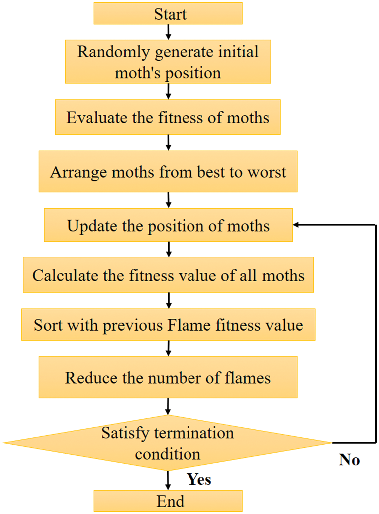
Figure 8: MFO flowchart

New in this study was the application of SMOGN and the four optimizers added to the architecture of the basic model, as shown in Fig. 9. The steps of reading and normalizing the datasets, the application of k-fold cross-validation and the division of data for training and testing are same as used in the basic models. Then the training data is divided into verification data and data optimized for SMOGN. The data after SMOGN is input to optimizers such as PSO, GA, GWO, and MFO for iteration, training results and verification data are used for prediction. The iterations were repeated until the best parameters were obtained. These were input to the best of the basic models, to make predication using the training results and validation data. The predicted results were stored and all the above-mentioned steps were repeated k times until the crossover was finished. The results were averaged and MAE, RMSE, and R2 were calculated. In this research, the Iteration of each optimizer will be set as 20 and the population will also be set as 20. On this basis, the parameters to be adjusted are the max depth, learning rate, and estimators. As for the parameter searching ranges, they will be set as [0.1, 0.5], [200, 550], and [2,6] respectively.

Figure 9: Architecture diagram of optimization model training

4  The Experimental Results

The first step is to perform k-fold cross-validation on the normalized parameters, dividing the input data into ten equal parts, one of which is used for validation and the rest for training. Next, normalization parameters were introduced into seven different trained models. Cross-validation was then done on these seven different algorithm models, and the corresponding parameters are set to determine the predicted results for each model. After the validation of the results, the accuracy of the models can be compared. The performance of each model is done by evaluating the MAE, RMSE, and R2 score which represents the relationship between the actual and predicted values.

MAE [33] is the average of the sum of the absolute value of the error between each actual value and the predicted value, which is a common evaluation indicator used in regression applications, the equation is shown below:

MAE=1n∑i=1n|yi−yi^|(12)

where n is the sample number, yi is the actual value of the ith data, and yi^ is the predicted value of the ith data. After acquiring the absolute value from the resulting “yi−yi^”, add them up and then divide them by “n” and the MAF is therefore obtained.

RMSE [33], also known as the standard error, is the square root of the error between the actual value and the predicted value. This algorithm is more sensitive to data errors and can be used to determine the dispersion level of data which allows better data prediction accuracy, the equation is shown below:

RMSE=1n∑i=1n(yi−yi^)2(13)

wherein n is the total number of predictions, yi is the actual value of the ith data, and yi^ is the predicted value of the ith data. It is similar to MAF, except that RMSE will be set as “yi−yi^”. After the square calculation, add them up and then divide them by “n”. Finally, acquire the square root for the result.

R2 score [33] is often used in regression model applications. The denominator is the square of the error between the actual value and the mean value, and its numerator is the square of the error between the actual value and the predicted value. Values are usually within a range of 0 ∼ 1. The higher the value the better the prediction accuracy of the model, the low value, on the other hand, or even an occasional negative value indicates a significant difference between the predicted result and the actual value of a model. The equation is shown below:

R2 ≡1−∑i=1n(yi−yi^)2∑i=1n(yi−y¯)2(14)

where n is the total prediction number, yi is the actual value of the ith data, yi^ is the predicted value of the ith data, and y¯ is the average of the data. Add up (yi−yi^)2  and then divide by the summation of (yi−y¯)2 to acquire the residual sum of squares. Next, deduct the residual sum of squares from “1”, and the result is the R2 value.

After training on the seven basic models, as stated in Section 3, was completed, the training results of the models, based on the above three evaluation indicators, are shown in Table 1. XGB, shows the lowest errors of MAE and RMSE, and the coefficient of determination R2 scored the closest to 1, the best performance amongst the basic models.

Finally, the distribution of actual and predicted values of the basic models were plotted as shown in Figs. 10–16. If an error of the predicted result was below 0.01, the color of that data point would be blue, between 0.01 and 0.02 green, and greater than 0.02 orange. It can be seen, from the ratio of blue to orange points in the figures, that XGB gives better performance than any of the others.

Figure 10: Adaboost prediction results: (a) comparison of actual and predicted values, (b) residual plot

Figure 11: MLP prediction results: (a) comparison of actual and predicted values, (b) residual plot

Figure 12: Densenet prediction results: (a) comparison of actual and predicted values, (b) residual plot

Figure 13: DT prediction results: (a) comparison of actual and predicted values, (b) residual plot

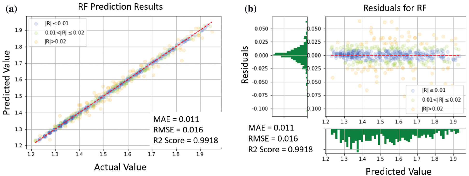
Figure 14: RF prediction results: (a) comparison of actual and predicted values, (b) residual plot

Figure 15: SVR prediction results: (a) comparison of actual and predicted values, (b) residual plot

Figure 16: XGB prediction results: (a) comparison of actual and predicted values, (b) residual plot

In this study, SMOGN and four optimizers were applied to the XGB model to improve accuracy. Fig. 17 shows the Learning Curve for these four optimizers. The vertical axis shows the Fitness Value concerning the evaluation indicator R2 score. As a better value is obtained by the optimizer, the Fitness Value will be updated. The fitness values obtained by the different optimizers are plotted in different colors. It can see that the MFO optimizer shows the best value, followed by GA, GWO, and PSO.

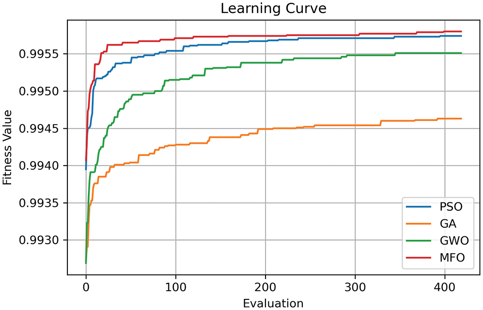
Figure 17: Learning curve

Fig. 18a shows a plot where SMOGN and the MFO optimizer were applied to the XGB model. A large number of blue points can be seen close to the line. This means the predicted values are very close to the actual values. In addition, it can also be seen in Fig. 18b that there are much smaller residual values than in the other models, and the distribution is close to 0. Moreover, Table 2 compares the basic models for SMOGN only with automatic parameter adjustment by an optimizer. It can be seen that there is improved performance in the MAE, RMSE, and R2 scores over that obtained by the basic models alone. The XGB model with SMOGN plus MFO optimizer gives the best performance.

Figure 18: SMOGN-MFO-XGB prediction results (a) comparison of actual and predicted values, (b) residual plot

5  Conclusion

The power factor of a motor evaluates its actual dissipated power. If the actual active power generated by a motor is close to the obtained power, then the power factor will be high. The closer it is to 1, the higher the efficiency of motor operation. The excitation current is a vital motor input parameter closely associated with the power factor. When a motor operates under load, it is typical for the power factor to fluctuate. The work done in this study was mainly intended to make it possible to predict the excitation current based on the input power factor, load current, and power factor error. This prediction allows the power factor to be changed by adjustment of the excitation current under a fixed input voltage and load.

In this study, load current, power factor, and power factor error data from a synchronous motor were pre-processed and introduced into seven different basic models for training and validated by the k-fold cross-validation method to improve data accountability. The accuracy of the predicted results showed that the XGB model gave the best performance. SMOGN, with four different optimizers, was then applied to XGB for training, and the final results are shown in Table 2, where the overall performance has been improved, especially with the MFO optimizer, to give MAE 0.0057, RMSE 0.0093, and an R2 score of 0.9973, as well as the lowest error and the highest accuracy. In conclusion, using the SMOGN-MFO-XGB optimization algorithm model derived in this study, it is possible to predict the required excitation current for operating a synchronous motor with the desired power factor under different loads. Adjustments to the excitation current can make these motors run more efficiently to reduce power loss and cost. Such a method can be used in a variety of applications like temperature rise prediction and the wearing prediction of machine tools. Experiments will be attempted in the future.

Funding Statement: This work was supported by the Ministry of Science and Technology, Taiwan, under Grants MOST 110-2221-E-194-037, NSTC 111-2823-8-194-002, 111-2221-E-194-052 and 11-2218-E-194-007.

Conflicts of Interest: The authors declare that they have no conflicts of interest to report regarding the present study.

Adaboost Model

Ensemble Learning [34] is training that integrates multiple supervised learning algorithms into one with improved learning accuracy. In addition, ensemble learning is further divided into stacking, bagging, and boosting. In this study, Adaboost [35] within boosting category is used as shown in Fig. 19, where multiple weak learners are integrated into series into one robust classifier. To start with, equal weights are assigned to each point of the dataset, then weak classifiers are identified and their weight is raised. Correctly classified points are identified, and their weight is reduced so that incorrect data can more easily to identify in the following classification. The number of weak learners is set to 50 in this study. If the setting is too tiny, underfitting can quickly occur.

Figure 19: Architecture diagram of Adaboost

MLP Model

MLP algorithm [36,37] is a three-layered artificial neural network, see Fig. 20. The three main layers are the input, hidden, and output layers. Iy, PF, and e from the dataset were fed into the input layer and then the hidden layers. Four hidden layers were used in this study, with 128, 64, 64, and 32 layers respectively. The nonlinear calculations of the different activation functions are carried out in these hidden layers, and the corresponding calculation results were fed into the output layer. In this study, the activation function in the hidden layers is set to Rectified Linear Unit (RELU), and the activation function of the output layer is set to Sigmoid for data normalization and output.

Figure 20: Architecture diagram of MLP

DenceNet Model

DenseNet [38] is a densely connected convolutional neural network, see Fig. 21, which is evolutionary like the Deep Neural Network Models ResNet [39] and GoogLeNet [40]. In ResNet, the model is deepened through shortcut connections, and the network degradation problems that affect performance are decreased by deepening. In GoogLeNet, the model is deepened and widened through structure inception, which solves the overfitting problem that arises when deepening is addressed. In the DenseNet applied in this study, the model enhances feature transmission through dense connection, where all the layers in the neural network were connected, and the input of each layer was mapped by extracting the features from all previous layers. The model solves the vanishing gradient problem, reduces model parameters to speed up calculation time, and most importantly, utilizes features more effectively to achieve better results.

Figure 21: Architecture diagram of DenseNet

Decision Tree Model

DT [41] as shown in Fig. 22, is further divided into a classification tree and regression trees. Datasets are located on the top of the tree, and data are directed into the lower branches according to their features or attributes. Further down the model becomes more complicated, and the final predicted values are much closer to the actual results. The significant difference between regression and classification trees is that a classification tree predicts discrete values while the regression number is a constant value. Since the problem to be addressed in this study was a regression type, a regression tree is chosen for prediction.

Figure 22: Architecture diagram of DT

The parameter setting of the maximum depth is set to 10 in this study, and the rest of the parameter values were preset. If no upper limit is set for the maximum depth, overfitting can quickly occur in this model.

Random Forest Model

RF [42] is composed of multiple DTs, see Fig. 23, but the DTs are not related to each other. Also, a Bootstrap Aggregation(Bagging) [43] is classified as ensemble learning. In this algorithm, samples all with the same weight are randomly selected during classification. Therefore, a sample may choose several to zero times. Samples are split into groups in each node by different attributes until no further split is possible. In addition, different DTs will be trained separately to obtain different predicted results. Finally, the biggest group among all results is obtained as the final output result. RF can get higher-dimensional data and reduce overfitting, so there is no need to set an upper depth limit. The accuracy of the prediction is maintained even if some features are missing. In this study, the parameters applied were default values, and the predicted results were better than those obtained with the DT.

Figure 23: Architecture diagram of RF

SVR Model

SVR [44] is a variation of the Support Vector Machine (SVM) [45]. SVM is a standard supervised learning algorithm where a plane is created, and data from the plane is classified accordingly. SVR creates a regression plane, as shown in Fig. 24, and sets a tolerance interval (ε) on both sides of a linear function. The interval is adjusted based on the differences between the data. Data close to the plane with no significant differences are considered a correct prediction. Data outside the dotted line are considered a loss. In this study, the penalty factor was set to 10. A more prominent penalty factor would mean that points far away from the plane would receive less attention. When points are close to infinity, there are fewer errors and correct predictions. However, a smaller penalty number, close to zero, means that meaningful predicted results cannot be obtained, overfitting would be a problem and the algorithm would not converge.

Figure 24: Architecture diagram of SVR

XGBoost Model

XGB [46,47] is an algorithm very similar to RF, wherein samples are randomly chosen by features during the decision-making through each tree. The difference between the two types is that there is no correlation between the trees in RF, and the predictions are carried out on multiple trees simultaneously. However, in XGB, there is a specific correlation between each tree, and the predictions are carried out on iterations one after the other, see Fig. 25. Any errors from the previous tree will be corrected. XGB combined the advantages of boosting and bagging in ensemble learning to obtain better model prediction and gives the most accurate predicted results achieved in this study, and the parameters applied were default values.

Figure 25: Architecture diagram of XGB

References

1. İ Çolak, R. Bayindir and Ö. Bay, “Reactive power compensation using a fuzzy logic controlled synchronous motor,” Energy Conversion Management, vol. 44, no. 13, pp. 2189–2204, 2003. [Google Scholar]
2. İ Çolak, R. Bayindir and İ Sefa, “Experimental study on reactive power compensation using a fuzzy logic controlled synchronous motor,” Energy Conversion Management, vol. 45, no. 15–16, pp. 2371–2391, 2004. [Google Scholar]
3. W. Hofmann, J. Schlabbach and W. Just, Reactive Power Compensation: A Practical Guide, Hoboken, New Jersey, U.S: John Wiley & Sons, 2012. [Online]. Available: https://www.pdfdrive.com/reactive-power-compensation-a-practical-guide-e185245978.html [Google Scholar]
4. T. Lu, Y. Wang, Z. Li, M. Li, W. Xu et al., “Reactive power compensation and control strategy for MMC-STATCOM doubly-fed wind farm,” in 2019 IEEE Innovative Smart Grid Technologies-Asia, Chengdu, China, pp. 3537–3542, 2019. [Google Scholar]
5. A. Dhaneria, “Grid connected PV system with reactive power compensation for the grid,” in 2020 IEEE Power & Energy Society Innovative Smart Grid Technologies Conf., Washington, DC, USA, pp. 1–5, 2020. [Google Scholar]
6. G. Valverde, E. Kyriakides, G. T. Heydt, and V. Terzija, “Nonlinear estimation of synchronous machine parameters using operating data,” IEEE Transactions on Energy Conversion., vol. 26, no. 3, pp. 831–839, 2011. [Google Scholar]
7. T. Senjyu, K. Kinjo, N. Urasaki and K. Uezato, “High efficiency control of synchronous reluctance motors using extended kalman filter,” IEEE Transactions on Industrial Electronics, vol. 50, no. 4, pp. 726–732, 2003. [Google Scholar]
8. R. Bayindir, S. Sagiroglu and I. Colak, “An intelligent power factor corrector for power system using artificial neural networks,” Electric Power System Research, vol. 79, no. 1, pp. 152–160, 2009. [Google Scholar]
9. H. T. Kahraman, R. Bayindir and S. Sagiroglu, “A new approach to predict the excitation current and parameter weightings of synchronous machines based on genetic algorithm-based k-NN estimator,” Energy Conversion and Management, vol. 64, pp. 129–138, 2012. [Google Scholar]
10. T. Niewierowicz, R. Escarela-Perez and E. Campero-Littlewood, “Hybrid genetic algorithm for the identification of high-order synchronous machine two-axis equivalent circuits,” Computers and Electrical Engineering, vol. 29, no. 4, pp. 505–522, 2003. [Google Scholar]
11. P. C. Sahu, R. C. Prusty and S. Panda, “MFO algorithm based fuzzy-PID controller in automatic generation control of multi-area system,” in 2017 Int. Conf. on Circuits Power and Computing Technologies, Kollam, India, pp. 1–6, 2017. [Google Scholar]
12. L. Wang, X. Wang, G. Liu and Y. Li, “Improved auto disturbance rejection control based on moth flame optimization for permanent magnet synchronous motor,” IEEJ Transactions on Electrical and Electronic Engineering, vol. 16, no. 8, pp. 1124–1135, 2021. [Google Scholar]
13. L. T. Le, H. Nguyen, J. Zhou, J. Dou and H. Moayedi, “Estimating the heating load of buildings for smart city planning using a novel artificial intelligence technique PSO-XGBoost,” Applied Science, vol. 9, no. 13, pp. 2714, 2019. [Google Scholar]
14. H. Jiang, Z. He, G. Ye, and H. Zhang, “Network intrusion detection based on PSO-xgboost model,” IEEE Access, vol. 8, pp. 58392–58401, 2020. [Google Scholar]
15. K. Song, F. Yan, T. Ding, L. Gao and S. Lu, “A steel property optimization model based on the XGBoost algorithm and improved PSO,” Computational Materials Science, vol. 174, pp. 109472, 2020. [Google Scholar]
16. UCI, “Synchronous machine data Set,” 2021. [Online]. https://archive.ics.uci.edu/ml/datasets/Synchronous+Machine+Data+Set [Google Scholar]
17. S. Sagiroglu, I. Colak and R. Bayindir, “Power factor correction technique based on artificial neural networks,” Energy Conversion Management, vol. 47, no. 18–19, pp. 3204–3215, 2006. [Google Scholar]
18. M. Kolarik, R. Burget and K. Riha, “Comparing normalization methods for limited batch size segmentation neural networks,” in 2020 43rd Int. Conf. on Telecommunications and Signal Processing, Milan, Italy, pp. 677–680, 2020. [Google Scholar]
19. D. Singh and B. Singh, “Investigating the impact of data normalization on classification performance,” Applied Soft Computing, vol. 97, Part B, pp. 105524, 2020. [Google Scholar]
20. P. Tamilarasi and R. U. Rani, “Diagnosis of crime rate against women using k-fold cross validation through machine learning,” in 2020 Fourth Int. Conf. on Computing Methodologies and Communication, Erode, India, pp. 1034–1038, 2020. [Google Scholar]
21. N. Almufadi and A. M. Qamar, “Deep convolutional neural network based churn prediction for telecommunication industry,” Computer System Science Engineering, vol. 43, no. 3, pp. 1255–1270, 2022. [Google Scholar]
22. S. Habib, S. Alyahya, A. Ahmed, M. Islam, S. Khan et al., “X-Ray image-based COVID-19 patient detection using machine learning-based techniques,” Computer System Science Engineering, vol. 43, no. 2, pp. 671–682, 2022. [Google Scholar]
23. P. Branco, L. Torgo and R. P. Ribeiro, “SMOGN: A pre-processing approach for imbalanced regression,” First Int. Workshop on Learning with Imbalanced Domains: Theory and Applications, Skopje, Macedonia, pp. 36–50, 2017. [Google Scholar]
24. H. Mesloub, M. T. Benchouia, R. Boumaaraf, A. Goléa, N. Goléa et al., “Design and implementation of DTC based on AFLC and PSO of a PMSM,” Mathematics Computers in Simulation, vol. 167, pp. 340–355, 2020. [Google Scholar]
25. V. Veeramanikandan and M. Jeyakarthic, “A futuristic framework for financial credit score prediction system using PSO based feature selection with random tree data classification model,” in 2019 Int. Conf. on Smart Systems and Inventive Technology, Tirunelveli, India, pp. 826–831, 2019. [Google Scholar]
26. S. Mirjalili, I. Aljarah, M. Mafarja, A. A. Heidari and H. Faris, “Grey wolf optimizer: Theory, literature review, and application in computational fluid dynamics problems,” in Nature-Inspired Optimizers, vol. 811. Cham, Switzerland: Springer, pp. 87–105, 2020. [Google Scholar]
27. F. K. Onay and S. B. Aydemı̇r, “Chaotic hunger games search optimization algorithm for global optimization and engineering problems,” Mathematics and Computers in Simulation, vol. 192, pp. 514–536, 2022. [Google Scholar]
28. S. Ardabili, A. Mosavi, S. S. Band and A. R. Varkonyi-Koczy, “Coronavirus disease (COVID-19) global prediction using hybrid artificial intelligence method of ANN trained with grey wolf optimizer,” in 2020 IEEE 3rd Int. Conf. and Workshop in Óbuda on Electrical and Power Engineering, Budapest, Hungary, pp. 000251–000254, 2020. [Google Scholar]
29. S. Cinaroglu and S. Bodur, “A new hybrid approach based on genetic algorithm for minimum vertex cover,” in 2018 Innovations in Intelligent Systems and Applications, Thessaloniki, Greece, pp. 1–5, 2018. [Google Scholar]
30. P. J. García-Nieto, E. García-Gonzalo, J. R. A. Fernández and C. D. Muñiz, “Modeling of the algal atypical increase in La barca reservoir using the DE optimized least square support vector machine approach with feature selection,” Mathematics and Computers in Simulation, vol. 166, pp. 461–480, 2019. [Google Scholar]
31. M. A. Elaziz, A. A. Ewees, R. A. Ibrahim and S. Lu, “Opposition-based moth-flame optimization improved by differential evolution for feature selection,” Mathematics and Computers in Simulation, vol. 168, pp. 48–75, 2020. [Google Scholar]
32. A. K. Kashyap, D. R. Parhi and P. B. Kumar, “Route outlining of humanoid robot on flat surface using MFO aided artificial potential field approach,” Proceedings of the Institution of Mechanical Engineers, Part B: Journal of Engineering Manufacture, vol. 236, no. 6–7, pp. 758–769, 2022. [Google Scholar]
33. D. Chicco, M. J. Warrens and G. Jurman, “The coefficient of determination R-squared is more informative than SMAPE, MAE, MAPE, MSE and RMSE in regression analysis evaluation,” PeerJ Computer Science, vol. 7, pp. e623, 2021. [Google Scholar] [PubMed]
34. Z. Zhu, Z. Wang, D. Li, Y. Zhu and W. Du, “Geometric structural ensemble learning for imbalanced problems,” IEEE Transactions of Cybernetics, vol. 50, no. 4, pp. 1617–1629, 2020. [Google Scholar] [PubMed]
35. S. Yadahalli and M. K. Nighot, “Adaboost based parameterized methods for wireless sensor networks,” in 2017 Int. Conf. on Smart Technologies for Smart Nation (SmartTechCon), Bengaluru, India, pp. 1370–1374, 2017. [Google Scholar]
36. K. Ucak, “A Runge-kutta MLP neural network based control method for nonlinear MIMO systems,” in 2019 6th Int. Conf. on Electrical and Electronics Engineering (ICEEE), Istanbul, Turkey, pp. 186–192, 2019. [Google Scholar]
37. F. V. Farahani, A. Ahmadi and M. H. F. Zarandi, “Hybrid intelligent approach for diagnosis of the lung nodule from CT images using spatial kernelized fuzzy c-means and ensemble learning,” Mathematics and Computers in Simulation, vol. 149, pp. 48–68, 2018. [Google Scholar]
38. K. Zhang, Y. Guo, X. Wang, J. Yuan and Q. Ding, “Multiple feature reweight DenseNet for image classification,” IEEE Access, vol. 7, pp. 9872–9880, 2019. [Google Scholar]
39. Z. Zhu, W. Zha, H. Liu, J. Geng, M. Zhou et al., “Juggler-ResNet: A flexible and high-speed ResNet optimization method for intrusion detection system in software-defined industrial networks,” IEEE Transactions on Industrial Informatics, vol. 18, no. 6, pp. 4224–4233, 2021. [Google Scholar]
40. Z. Zhu, J. Li, L. Zhuo and J. Zhang, “Extreme weather recognition using a novel fine-tuning strategy and optimized GoogLeNet,” in 2017 Int. Conf. on Digital Image Computing: Techniques and Applications (DICTA), Sydney, NSW, Australia, pp. 1–7, 2017. [Google Scholar]
41. J. Mrva, S. Neupauer, L. Hudec, J. Sevcech and P. Kapec, “Decision support in medical data using 3D decision tree visualisation,” in 2019 E-Health and Bioengineering Conf. (EHB), Iasi, Romania, pp. 1–4, 2019. [Google Scholar]
42. H. Lan and Y. Pan, “A crowdsourcing quality prediction model based on random forests,” in 2019 IEEE/ACIS 18th Int. Conf. on Computer and Information Science (ICIS), Beijing, China, pp. 315–319, 2019. [Google Scholar]
43. Y. Yu and H. Su, “Collaborative representation ensemble using bagging for hyperspectral image classification,” in IGARSS 2019–2019 IEEE Int. Geoscience and Remote Sensing Symp., Yokohama, Japan, pp. 2738–2741, 2019. [Google Scholar]
44. D. Wu and S. Wang, “Comparison of road traffic accident prediction effects based on SVR and BP neural network,” in 2020 IEEE Int. Conf. on Information Technology, Big Data and Artificial Intelligence (ICIBA), Samara, Russia, pp. 1150–1154, 2020. [Google Scholar]
45. H. Xiangdong and W. Shaoqing, “Prediction of bottom-hole flow pressure in coalbed gas wells based on GA optimization SVM,” in 2018 IEEE 3rd Advanced Information Technology, Electronic and Automation Control Conf. (IAEAC), Chongqing, China, pp. 138–141, 2018. [Google Scholar]
46. M. Mishra, B. Patnaik, R. C. Bansal, R. Naidoo, B. Naik et al., “DTCDWT-SMOTE-XGBoost-based islanding detection for distributed generation systems: An approach of class-imbalanced issue,” IEEE Systems Journal, vol. 16, no. 2, pp. 2008–2019, 2021. [Google Scholar]
47. S. J. Kumar, U. Maheswaran, G. Jaikishan and B. Divagar, “Melanoma classification using XGB classifier and EfficientNet,” in 2021 Int. Conf. on Intelligent Technologies (CONIT), Karnataka, India, pp. 1–4, 2021. [Google Scholar]
AppendixAdaboost Model