FST-EfficientNetV2: Exceptional Image Classification for Remote Sensing

1  Introduction

Remote sensing is the primary method for humans to observe the Earth from space, and the interpretation of RSI is crucial in data analysis [1]. As the number of orbital sensors has increased year by year, the data volume of the RSI has grown too large to interpret all by hand. As a result, the automatic analysis of RSI using a machine learning (ML) algorithm has been an active research field for the past two decades [2]. However, the traditional ML-based algorithm has been heavily reliant on human-engineered techniques for feature extraction. Hence, the RSI tasks are labor-intensive even when using ML algorithms. Fortunately, much of this has changed with the recent availability of DL [3]. The distinctive advantages of DL, i.e., automatic feature extraction, end-to-end training procedures, and higher accuracy, correspond to less labor, less domain-expert dependence, and better performance. As a result, the DL method has quickly dominated the research field of RSI [4].

There are different applications of DL methods for RSI, i.e., SC [5], semantic segmentation [6,7], object detection [8,9], and change detection [10]. SC is the fundamental application, owing to the fact that its feature extraction is the basis of the others. As the algorithm’s engine, a series of DL models have been demonstrated for RSI-SC in the past five years [11], e.g., deep belief networks, auto-encoders, generative adversarial networks, and deep CNNs. Gradually, the CNN outperforms the others due to its better performance and efficiency. With the bloom of CNN, a lot of approaches have been demonstrated for RSI-SC. However, if evaluated from today’s perspective, many of them are not ideal because of the insufficient accumulation of knowledge in the short term. Meanwhile, traditional ML algorithmic ideas have had a negative impact on their successors to some extent.

Firstly, the CNN model is only treated as a fixed deep feature extractor for traditional ML classifiers owing to the lack of large-scale RSI datasets [12–14]. That is, the CNN model is only pre-trained on natural image datasets but not on the ones from RSI. As a result, the superior representation-extracting ability of CNN is totally abandoned. These approaches’ performance is very limited to date, despite outperforming the previous ML-based ones. Secondly, several large-scale RSI datasets have been released since 2018. Then, the novel CNN-based approaches are commonly trained on the RSI datasets. Due to a lack of insight into CNN's superior representation ability, handcrafted features are intensively fused with deep features for the purpose of achieving higher accuracy. Except for acceptable accuracy, these algorithms exhibit multiple stages and complex expert knowledge, making the entire method more complex. Furthermore, a combination or an ensemble of CNNs has been widely employed for the accuracy contest of the RSI-SC. In terms of accuracy, the ensemble is the best, and the other combination ones are commonly better than previous fusion algorithms. However, multi-stage and multi-model strategies are common in these methods, which correspond to higher hardware budgets. More importantly, these algorithms are not completely end-to-end.

The success of DL mainly results from the automatic feature extraction and the end-to-end training procedure. It replaces the labor-intensive process of feature engineering and reduces the reliance of traditional ML on domain-expert knowledge. Moreover, an abundance of datasets and computational resources for DL is vital, too. Now, computation acceleration in DL is commonly implemented through GPUs, where accessible hardware (e.g., video memory) is always fixed and expensive. To some extent, algorithms do not need to consider hardware budgets for academic purposes. Conversely, algorithms with higher GPU costs, e.g., the ensemble and other combinations of CNNs, are not suitable for routine tasks, especially for industrial implementations. Meanwhile, the fusion types still have too much domain-specific experience, which limits the development of DL. Furthermore, all the aforementioned methods are not completely end-to-end, which corresponds to the lack of an automation advantage. In conclusion, all the previous methods have lost the key advantages of DL, i.e., automation and simplicity.

There is a way to achieve higher accuracy with a simpler procedure and a controllable hardware cost. As the author's prior study concluded [15], the performance of the CNN algorithm for RSI-SC can be noticeably improved by only using a single model coupled with a proper training optimization strategy. The proposed FST-EfficientNet is a fast and simple training framework that only consists of one CNN model and is totally one-stage and end-to-end without any handcrafted features or discriminators. Meanwhile, it is a state-of-the-art (SOTA) approach that has outperformed all the prior methods on two classic benchmark datasets. Nevertheless, the author’s recent research finds the FST-EfficientNet algorithm is not perfect somehow. The reasons are as follows: Firstly, the algorithm’s best accuracy relies on higher testing resolutions, e.g., the resolutions of 5122 and 6002, which limit industrial implementations within a restricted hardware budget. Secondly, its performance can be noticeably improved with very limited growth in GPU budgets if some algorithmic modifications and hyper-parameter re-optimizations are made.

Motivated by the above ideas, the author proposes a novel CNN-based framework named FST-EfficientNetV2. The algorithm has fast, simple, and more lightweight characteristics. It is more efficient in training and has better testing accuracy than its predecessor. Meanwhile, the time and hardware costs of the GPU are reduced by 4–5 times compared to its predecessor. In addition, the automation, simplicity, and lower reliance on specific knowledge of its predecessor are retained. That is, the FST-EfficientNetV2 is still a standard and simple transfer learning strategy, with the base EfficientNetV2-S model unchanged [16]. The three contributions of this study are summarized as follows:

Firstly, FST-EfficientNetV2 is a novel CNN-based approach that achieves SOTA performance with a 0.3%–1.1% increase in accuracy over its predecessor. The algorithm still employs a routine transfer learning strategy. The model has fewer parameters, at about 22 megabytes (M) with 8.8 billion (B) floating-point operations (FLOPs), and the whole algorithm flowchart is understandable.

Secondly, FST-EfficientNetV2 is more efficient than its predecessor, with higher accuracy and 4–5 times lower GPU and time costs. In particular, the FST-EfficientNetV2 method has achieved an amazing performance with a 1.7%–6.2% increase in accuracy over the other previous SOTA approaches for RSI-SC. Furthermore, the whole framework nearly requires no domain-expert knowledge in remote sensing. This novel algorithm is more suitable for industrial implementations within a restricted hardware budget.

Finally, and most importantly, the FST-EfficientNetV2 practice shares a novel idea for improving the performance and efficiency of CNN methods for RSI-SSC. On the one hand, the results suggest that it is unnecessary to give up the advantages of DL (i.e., simplicity and automation) for the pure purpose of higher accuracy. On the other hand, the author argues that the distribution shift introduced by DA is vital to the method’s performance. It should not be ignored in our feature work.

The remainder of this paper is organized as follows: Section 2 gives a brief review of related works. Section 3 describes the proposed method in detail. Section 4 introduces experimental designs and results. Experimental results are discussed in Section 5. Section 6 presents a conclusion and future work.

2  Related Works

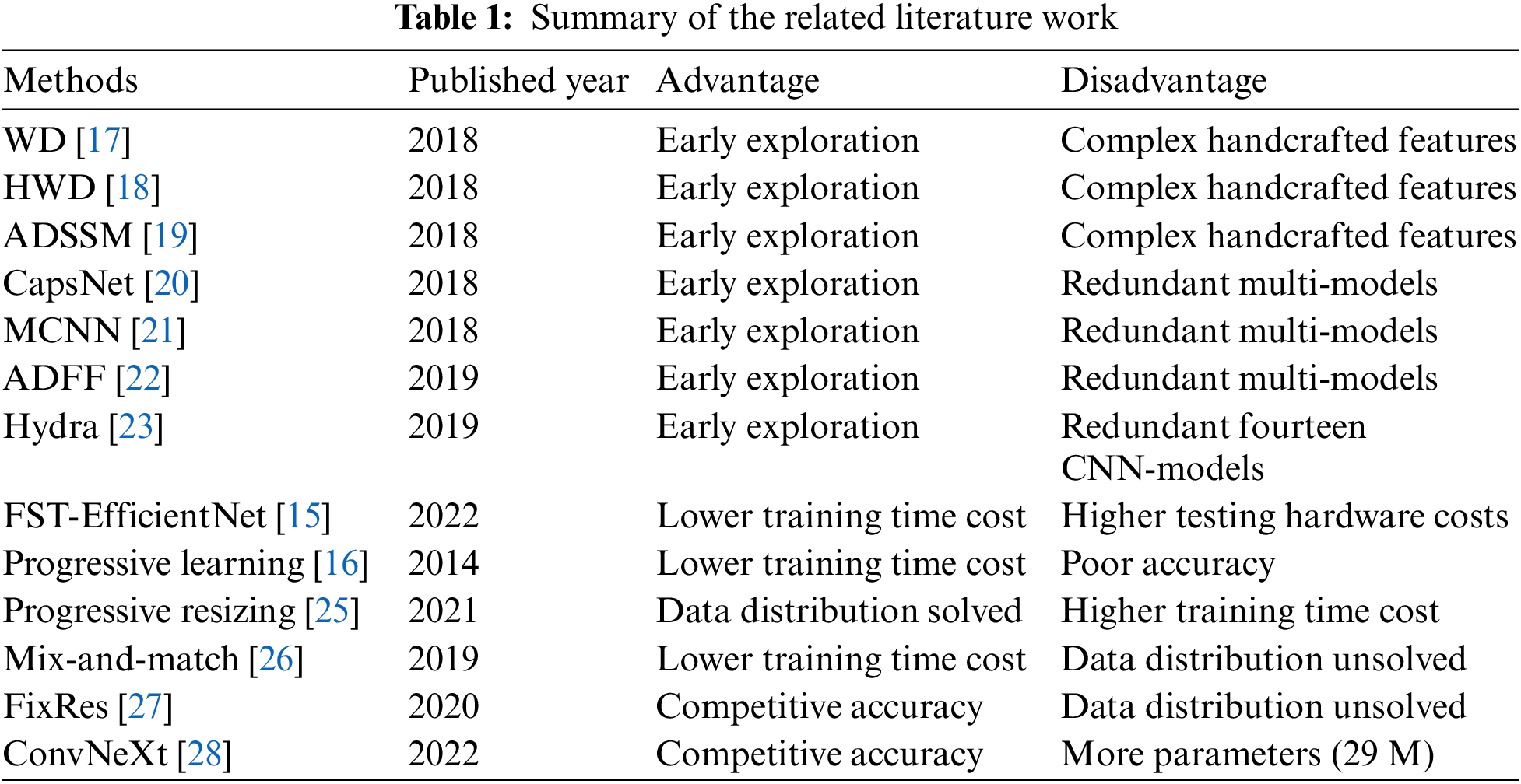
Firstly, the fusion of deep CNN features with handcrafted ones is the dominant technical route, which makes the algorithms very complex. Liu et al. fuse deep features of CNNs with handcrafted ones (i.e., the Wasserstein distance, WD) for SC tasks [17]. Then they propose the hierarchy Wasserstein distance (HWD) as an update of the former [18]. Zhu et al. also propose a fusion algorithm [19]. The deep features of a Caffe CNN are fused with handcrafted features from an adaptive deep sparse semantic modeling (ADSSM) framework.

Secondly, multi-models or ensembles of CNNs have been widely tested for the RSI-SC accuracy contest. Zhang et al. propose a cascade algorithm that employs two CNNs (i.e., a VGGNet-16 and an Inception-V3) as feature extractors for the feed into a capsule network (CapsNet) [20]. To improve the robustness of scale variation, Liu et al. also propose a two-branch algorithm that employs a multi-scale CNN (MCNN) and a fixed-scale CNN (i.e., two AlexNets) [21]. Similarly, Zhu et al. propose an attention-based deep feature fusion (ADFF) algorithm that consists of two residual CNNs (ResNet), one as a deep feature extractor and the other as a gradient-attention generator [22]. Ultimately, Minetto et al. demonstrate the “Hydra” algorithm, which consists of fourteen ResNets and dense CNNs in an ensemble [23]. In terms of accuracy, the Hydra is the best, and the other three are commonly better than previous fusion algorithms. However, these algorithms seldom consider the hardware costs.

Ample data is essential for DL-based algorithms. However, acquiring a larger-scale dataset for specific-domain tasks is always difficult. Hence, DA and transfer learning strategies are commonly employed in the training optimization process of DL [24]. Theoretically, DA solves the data-insufficiency problem in DL as the labeled dataset does, but the time cost of training also climbs as the quantity of samples increases. Therefore, the optimization strategy for fast training is an active research field in DL.

As a pioneer, Howard proposes a “progressive resizing” method by increasing image size in successive training epochs [25]. Smaller image sizes correspond to less computation and memory consumption on GPUs. The concept will significantly reduce the time required for training. However, the method's testing accuracy is lower than the traditional ones with a fixed-size strategy. Fundamentally, this mainly stems from the fact that the augmented samples lead to a distribution shift compared to the original dataset. That is, different distributions in training and testing data have reduced the model's performance.

Similarly, Hoffer et al. propose a “mix-and-match” method by using stochastic images and batch sizes through random sampling to improve the training speed [26]. The method does work to some extent. However, the distribution shift is still unsolved. That is due to the fact that routine cascade DA strategies always include a random image-resizing operation ahead of the mix-and-match operations. So the randomly resized images still introduce a distribution shift into the training process. Similarly, Tan et al. also propose a “progressive learning” method while the EfficientNetV2-S models are released. That is, the training image size progressively increases, coupled with more intensive regularization. Stronger regularization can somehow correct distribution shifts, but higher time costs are always associated.

Finally, Touvron et al. demonstrate the existence of a distribution shift between training and testing data, which comes from the random size crop (RSC) transformation, and then propose the “FixRes” method as a solution [27]. In particular, they find that the ratio of the training and testing image sizes is crucial if the RSC operation is used for training images. That is, there is an empirical ratio that can employ smaller training images and larger testing ones, which results in higher accuracy and lower time costs. Smaller images produced by the RSC have a data distribution similar to larger ones.

Additionally, some of the latest ideals concerned with CNN’s training optimization have been demonstrated in the “ConvNeXt” work, which can systematically boost the model’s accuracy in image classification [28]. That is, the AdamW optimizer [29] and label smoothing (LS) technique [30] of the loss function are more efficient for CNN’s training optimization strategy. It is known that the AdamW is less sensitive to the learning rate, while the LS can help DL-based models achieve higher accuracy compared to the fixed one-hot label. In particular, the applications of AdamW and LS have no additional cost on the GPU. To the best of the author’s knowledge, the combination of AdamW and LS has never been tested for RSI-SC. The summary of the related literature work is presented in Table 1.

Motivated by all the above ideas, the author first proposed the former STOA FST-EfficientNet for RSI-SC in the DL community. In more detail, a fixed empirical ratio of image size is uniformly employed during the training and testing phases for all different testing resolutions. However, this one-ratio-for-all strategy is not ideal somehow. To be precise, the optimal size of training images transformed by the RSC should be re-determined if the testing resolution changes. Meanwhile, the FST-EfficientNet employs bigger testing resolutions of 5002 and 6002, which correspond to higher GPU budgets and training time costs. To be honest, the testing resolution of 2562 should be more common and less expensive in terms of routine GPU budgets.

Therefore, in this paper, the author proposes a novel algorithm for acquiring the empirical ratio more accurately. First of all, the Adam-W algorithm and LS technique are also employed in the optimization strategy for hyperparameters. In more detail, previous ideals like feature fusion, multi-models, or ensembles of CNNs are totally excluded in this paper. Furthermore, the “progressive resizing,” “mix-and-match,” and “progressive learning” methods are excluded in view of their time cost and unsolved data distribution. As the ConvNeXt architectures have more parameters, the EfficientNetV2-S model is unchanged in this paper. Finally, only part of the “FixRes” ideal is employed in this paper. That is, only the RSC transformation is conducted in the DA strategies, but no layer is frozen as the RSI dataset is smaller compared to the natural image ones. As the most obvious improvement, a customized empirical ratio for the RSI dataset is included in this paper. As a result, this study achieves a lightweight framework that is both efficient and easy to implement.

3  Methodologies

3.1 Model Architecture

The proposed FST-EfficientNetV2 is a one-stage and end-to-end framework that uses a classical transfer-learning strategy without any handcrafted features. At the start of the pipeline, data augmentation consisting of routine transformations is applied to the input image, and then the transformed image is fed into the base model (i.e., the EfficientNetV2-S). In 2021, the EfficientNetV2 architectures outperformed the competition on ImageNet2012. The EfficientNetV2-S is the baseline model, and its architecture consists of two different conv blocks, i.e., the MobileNet conv (MBC) [31] and fused MobileNet conv (FMBC) [32].

The framework of FST-EfficientNetV2 and the structural differences between MBC and FMBC are shown in Fig. 1. There are two structural differences between the MBC and FMBC. Firstly, the depth-wise separable Conv block (i.e., a 1 × 1 Conv layer followed by a depth-wise 3 × 3 one) of MBC is replaced by a single regular 3 × 3 Conv layer. Secondly, the squeeze-and-excitation (SE) block [33], which improves CNN performance via the channel attention mechanism, is also excluded from the FMBC. Since the convolutional operation is obviously reduced in the FMBC, the EfficientNetV2-S is a lightweight model with only 22M parameters and 8.8B FLOPs.

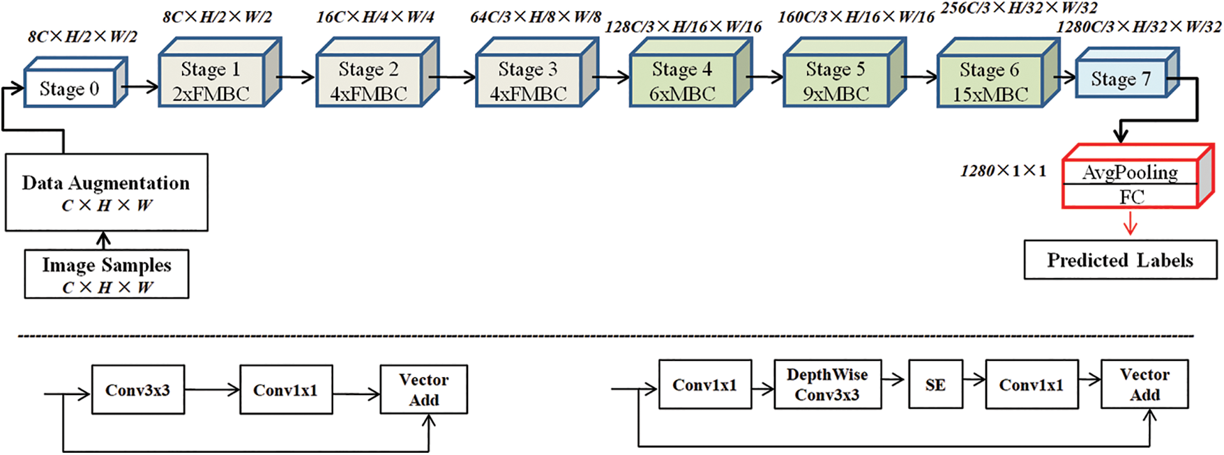
Figure 1: Framework of FST-EfficientNetV2 with structural differences between MBC and FMBC

As shown on the top of Fig. 1, the model’s architecture consists of seven stages, an AvgPooling layer, and a fully connected (FC) layer. The number of FMBC in Stage 1, Stage 2, and Stage 3 is 2, 4, and 4, while the number of MBC in Stage 4, Stage 5, and Stage 6 is 6, 9, and 15. The EfficientNetV2-S model employs the default ones in PyTorch. Note that only the FC layer is replaced according to different datasets.

3.2 Algorithm Update

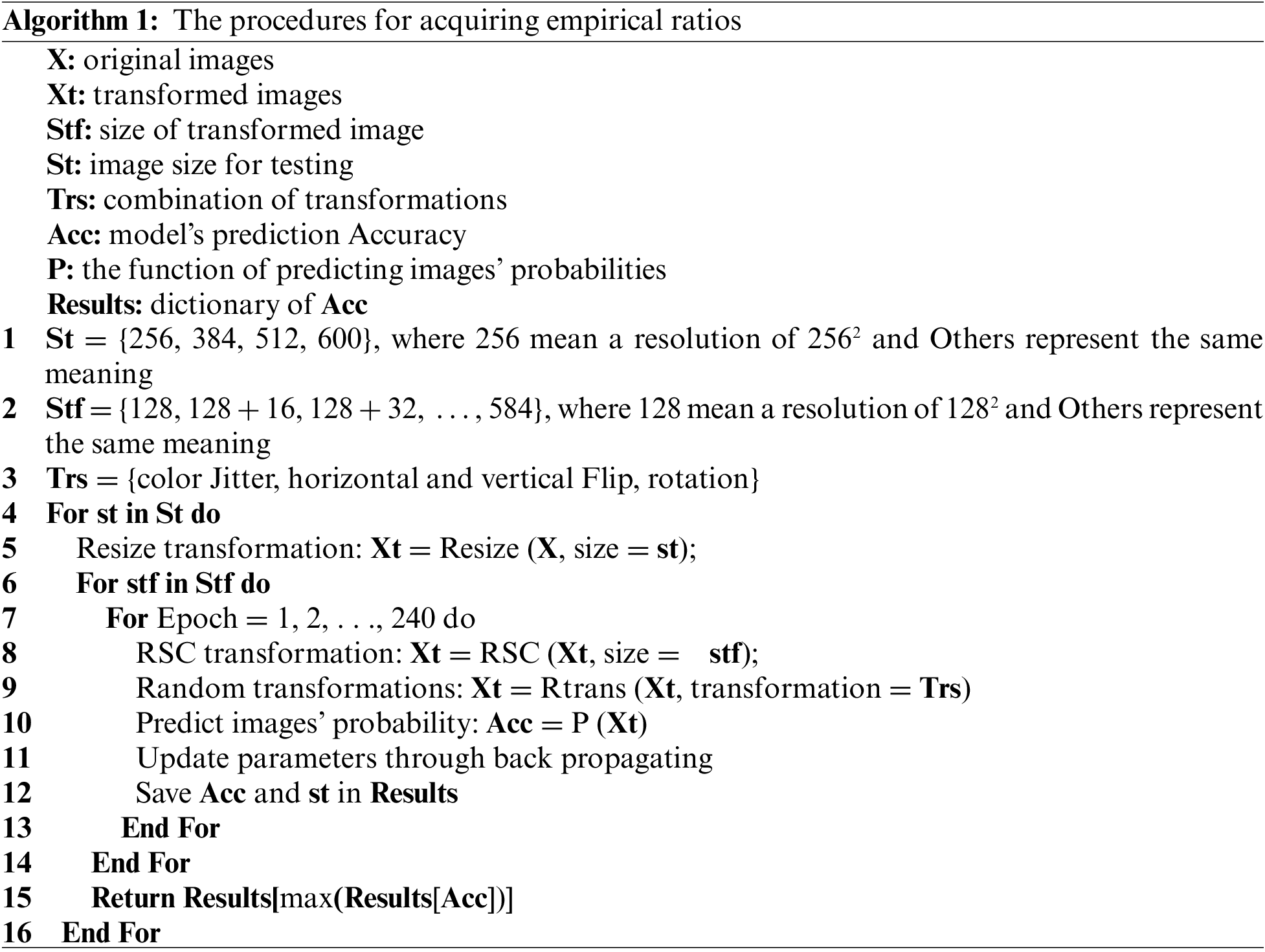
Algorithm 1 presents the procedures for acquiring the empirical ratio, at which the images generated by the RSC have a more similar distribution to the original ones. It is well known that an image with a higher resolution has more information. Since the original resolutions are varied, the characteristics of the data distribution in every RSI dataset are different. Meanwhile, the “FixRes” study also proves that the empirical ratio results for different testing sizes are different even for the same dataset. To solve this problem, the empirical ratios of FST-EfficientNetV2 have been re-determined for all testing resolutions in every dataset.

Additionally, some hyperparameters are reset for the FST-EfficientNetV2 training strategy. Firstly, the initial learning rate (LR) is reduced by 10 times. The former LR of 0.001 is slightly large for transfer learning. In transfer learning, the iterative process is typically smoother with a lower LR. Secondly, the LS technique is employed for the cross-entropy loss function. The LS value is now 0.1 instead of the former zero. Thirdly, the Adam-W is used instead of the former stochastic gradient descent as the optimizer of the error back-propagation algorithm. The weight decay value is 0.01. Fourthly, a differential training epoch of 120–180 is used in Step 1. The benchmark datasets have a distinct difference in the volume of samples. Commonly, the smaller ones need more iterative steps until model convergence. Finally, a training batch size of 30 is used for all testing resolutions to validate the method’s generalization. A gradient accumulation trick is employed for the training of larger images, if necessary.

3.3 Algorithm of Model Training

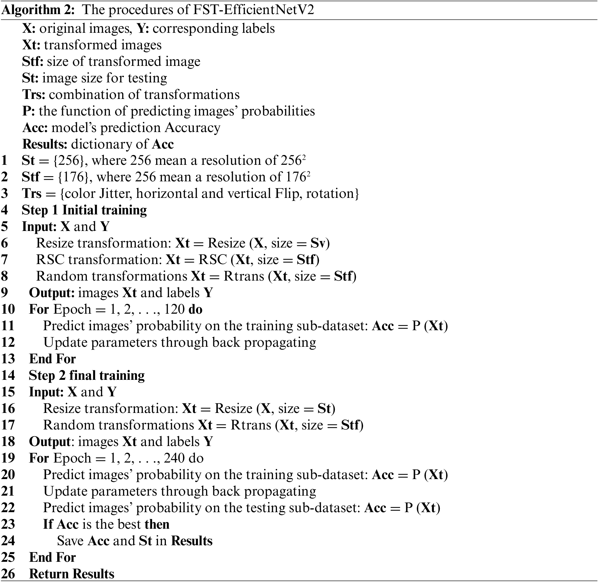
The algorithm of the FST-EfficientNetV2 framework is shown in Algorithm 2. In detail, there are several updates to the algorithm compared to its predecessor. To begin, without any testing procedure or frozen layer, the Step 1 training epoch is 120. The 180 epochs of Step 1 are only used on the smaller dataset. Secondly, the size of the training image transformed by the RSC is re-obtained and notably smaller. Thirdly, the initial learning rate is 0.0001 for Step 1 and 0.0001 for Step 2, both with cosine decay. Fourthly, the batch size is a consistent 30 compared to the former's halved one. That is, the total number of iterations is basically the same as its predecessor. Fifthly, the testing epoch is set at an empirical 240. Extensive, repeated experiments have shown the model usually achieves the best accuracy in the interval of 160 to 220. Finally, and more crucially, the testing resolution is reduced from 512 and 600 to 256. It corresponds to 3–5 times the savings in the GPU and time costs.

3.4 Data Augmentation

The DA in this study employs the same strategy as the former FST-EfficientNet, which consists of six kinds of image transformations in a cascade combination. That is, the resize is followed by the RSC, and then there is the color jitter, horizontal flip, vertical flip, and rotation in turn. The RSC is still excluded from Step 2. The implementation of data augmentation is performed on the central processing unit (CPU) via the default code in the PyTorch libraries.

3.5 Dataset and Division

There are two benchmark RSI datasets used in this study, i.e., the Aerial Image Dataset (AID) [34] and the Northwestern Polytechnic University Remote Sensing Image Scene Classification 45 Dataset (NWPU45D) [35]. These two datasets were both cropped from Google Earth images and released in 2017. In details, AID has 30 scene subclasses and 10,000 images with a fixed resolution of 6002 pixels, while NWPU45D has 45 subclasses and 31,500 images with a fixed resolution of 2562 pixels. Additionally, AID has 220–420 images per subclass, while NWPU45D has 700 images per subclass. The typical samples from the two datasets are shown in Fig. 2.

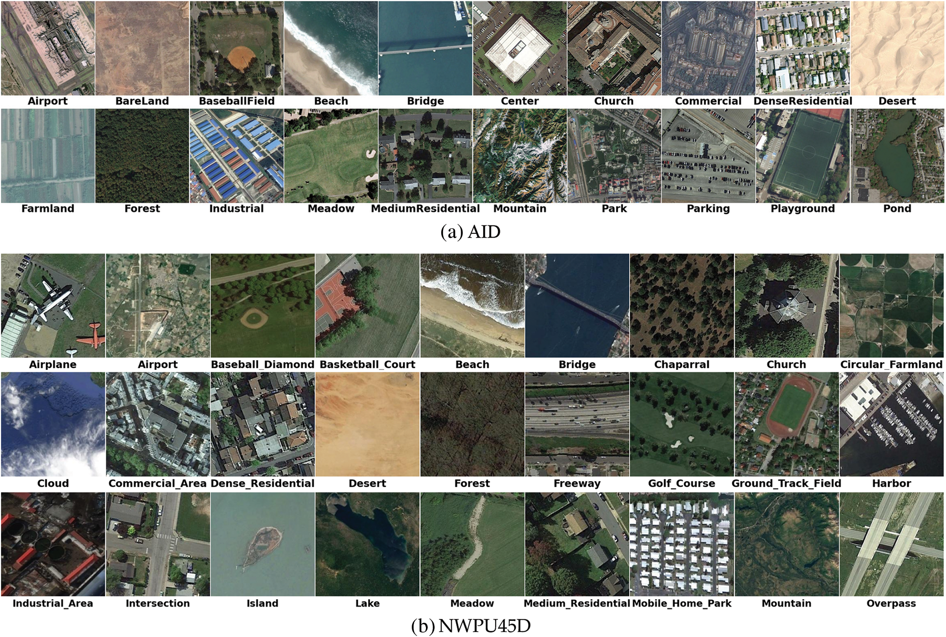
Figure 2: Typical samples of the AID and NWPU45D

AID and NWPU45D have been widely used as benchmarks in previous studies. The overall accuracy (OA) and confusion matrix are commonly used as criteria for methods' performance evaluation. In detail, the OA is as described in Eq. (1):

OA=Nc/Nt(1)

The OA is defined as the total number of accurately classified samples (Nc) divided by the total number of tested samples (Nt).

The confusion matrix is a specific table of the detailed classification result, which visualizes the algorithm's performance. Each row of the matrix represents the sample in an actual class, while each column represents the sample in a predicted class. That is, for each element Xij (i represents lines, and j represents rows) in the table, it presents the proportion of the predicted images in the ith category that actually belong to the jth class.

Additionally, the training ratios of the two datasets are the same with FST-EfficientNet, i.e., 20% and 50% for AID and 10% and 20% for NWPU45D. The training and testing subsets are completely the same, too.

3.6 Hardware and Software Environments

The experiments were performed on three personal computers equipped with an AMD 5700X CPU, a RTX 2060 GPU with 12 gigabytes (GB) of video memory, and 32 GB of system memory, running PyTorch 1.11.0 with the Compute Unified Device Architecture 11.5 on Win10. The base model is pre-trained on ImageNet 2012. All the experimental results were also averaged over three runs.

4  Results

4.1 Empirical Ratios

The OA results from different RSC sizes of AID are shown in Fig. 3. As shown in Fig. 3a, the OA shows a similar rapid increase as the RSC size increases in Step 1 if the RSC size is below 208. Then, the OA still shows a moderate increase (except for the testing resolution of 2562) when the RSC size is above 208. However, the result in Step 1 is not a guarantee of better accuracy in Step 2. As shown in Fig. 3b, the OA probably shows better accuracy at a smaller RSC size if the model has been trained at a testing resolution for 24 epochs. More specifically, the RSC size of 208 used in FST-EfficientNet is only acceptable for the testing process at a resolution of 3842. The results prove the “one-size-fits-all” strategy used in the author’s prior study has led to a suboptimal starting point for Step 2, except for the testing resolution of 3842. Therefore, the empirical ratios (i.e., the RSC size for Step 1) of AID are re-determined in the interval of 96–240. Finally, the RSC size is reset to 176 for the testing resolution of 2562.

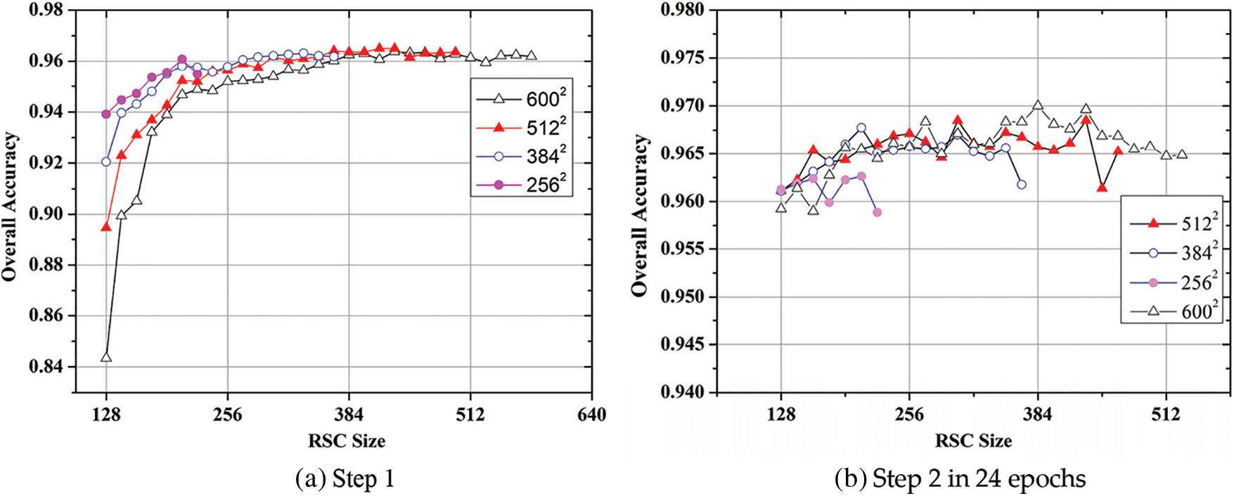
Figure 3: OA results from different RSC sizes of AID

In addition, the empirical ratios of NWPU45D are similar to the AID results, and the experiential figure is not presented to save space. The RSC size for Step 1 of NWPU45D is reset at 176 for the testing resolution of 2562, too. Generally, as the author concludes in FST-EfficientNet, a minor improvement in accuracy is observed when the testing resolution is increased above 2562. Therefore, the FST-EfficientNetV2 is only designed for the testing resolution of 2562 on AID and NWPU45D. In other words, the testing resolution is reduced from 6002 to 2562 on AID, which is an 81.8% decrease in GPU budget. On the other hand, a significant 75% decrease is shown on NWPU45D for the reduction of testing resolution from 5122 to 2562.

4.2 OA on AID

The OA results of the FST-EfficientNetV2 and other methods on AID are shown in Table 2, where the results of the testing resolutions of 2562 and 6002 are listed for the FST-EfficientNetV2 and its predecessor. In the column of training ratio (20%), the OA of FST-EfficientNetV2 shows a noticeable advantage over other methods with a 3.1% increase. If compared to its predecessor, FST-EfficientNetV2 still shows a remarkable increase in OA of 0.3%–0.9%. In the column of training ratio (50%), the OA of FST-EfficientNetV2 shows a noticeable advantage over other methods with a 0.9%–6.2% increase. However, FST-EfficientNetV2 only shows a minor increase of 0.6% over its predecessor at the testing resolution of 2562. Nonetheless, when the following factors are considered, the FST-EfficientNetV2 does outperform its predecessor:

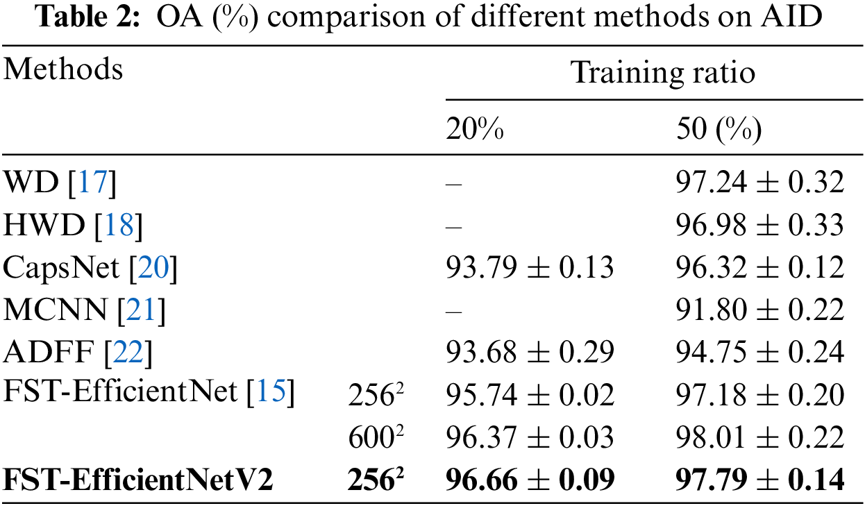
Firstly, there is always artificial noise and a covariate shift in the dataset. The OA of 97.79% of FST-EfficientNetV2 is very close to the 98.01% of its predecessor at the testing ratio of 50%. Secondly, the FST-EfficientNetV2 employs a noticeably smaller resolution of 2562 than its predecessor, which is one of 6002. The FST-EfficientNetV2 consumes 81.8% less GPU memory, and its training is five times faster than that of its predecessor. More crucially, even if tested at a resolution of 2562, the FST-EfficientNetV2 still performs better with fewer training samples than its predecessor, which is one of 6002. It indicates that FST-EfficientNetV2 has better representation ability.

Therefore, FST-EfficientNetV2 is a novel SOTA method for the classification of AID. In terms of GPU budget and time cost, the algorithm is faster and less expensive.

4.3 Confusion Matrixes of AID

The confusion matrixes of AID at 20% training ratios are shown in Fig. 4. There are 4 subclasses, including the forest, mountain, railway station, and viaduct, with an OA of 100%. Besides, there are 13 subclasses with an OA above 98%. The confusion mainly occurs in the subclasses, including the center, park, resort, and school. In detail, the center is frequently confused with square, while the subclass for school is the commercial area. In particular, the park and square are frequently confused with each other.

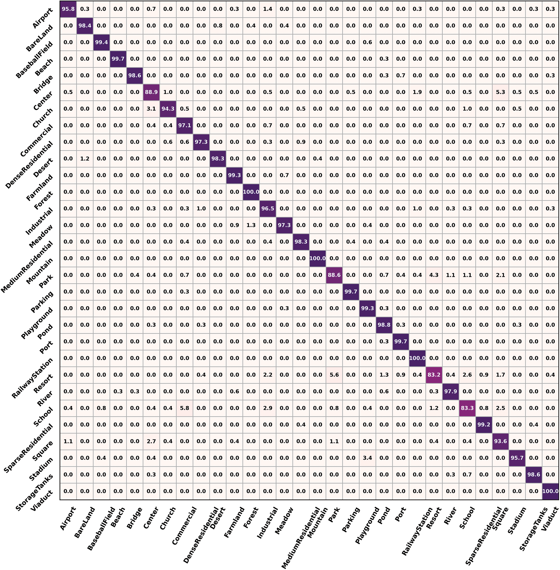
Figure 4: Confusion matrixes of AID at 20% training ratios

The confusion matrixes of AID at 50% training ratios are shown in Fig. 5. There are 6 more subclasses, including the baseball field, beach, desert, farmland, meadow, and parking, with an OA of 100%. In total, there are 22 subclasses with an OA above 98%. The confusion mainly occurs in the same subclasses as those in Fig. 4a. However, the OA results of these four subclasses have increased by 5% when compared to the previous ones.

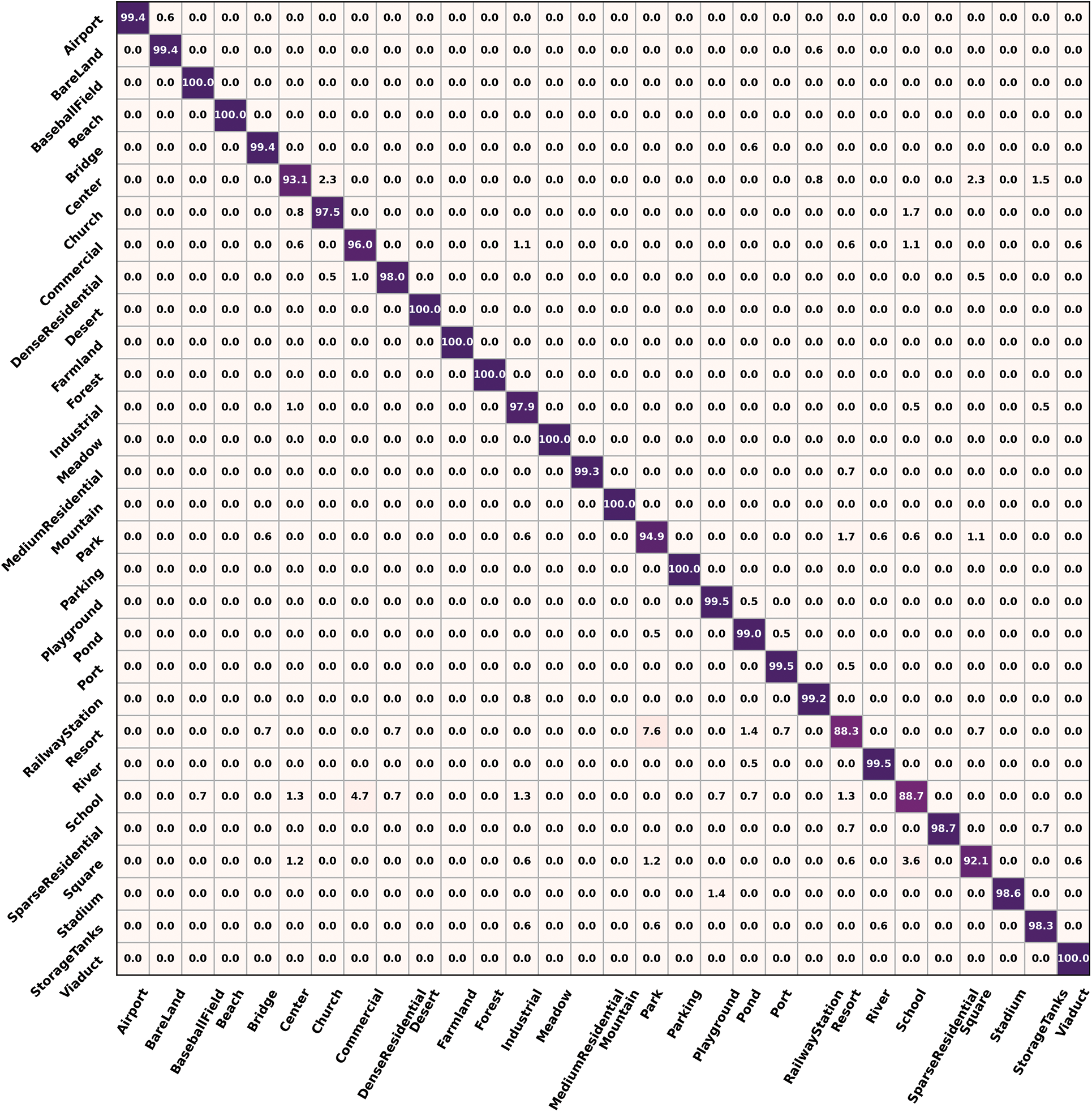
Figure 5: Confusion matrixes of AID at 50% training ratios

In brief, the confusion results of FST-EfficientNetV2 are consistent with its predecessor and other prior studies. Unlikely, the OA results of FST-EfficientNetV2 are much better than the other prior methods. Meanwhile, the FST-EfficientNetV2 has shown a significant improvement in OA by using fewer training samples.

4.4 OA on NWPU45D

The OA results of the FST-EfficientNetV2 and other methods on NWPU45D are shown in Table 3, where the results of the testing resolutions of 2562 and 5122 are listed for the FST-EfficientNetV2 and its predecessor. In the column of 10% training ratio, the OA of FST-EfficientNetV2 shows a noticeable advantage over other methods with a 1.8%–5.2% increase. Over its predecessor, FST-EfficientNetV2 still shows a remarkable increase in OA of 0.9%–1.1%.

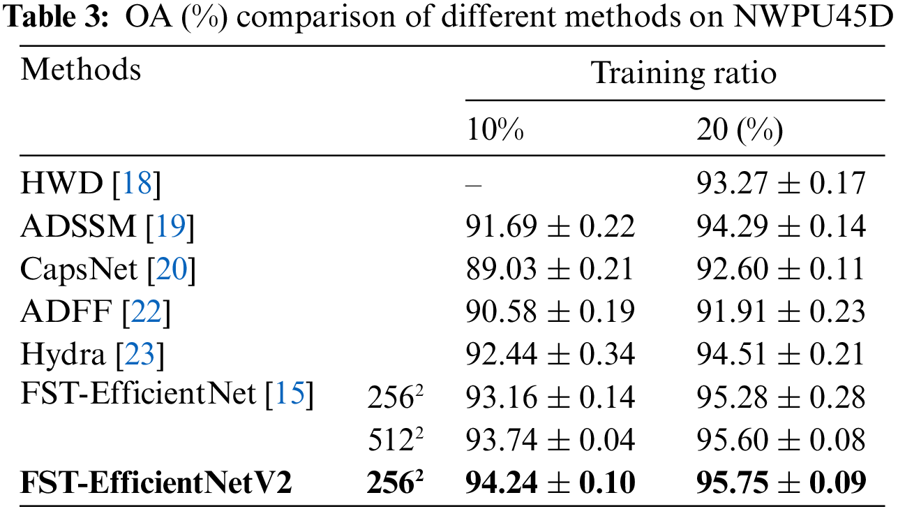
In the column of 50% training ratio, the OA of FST-EfficientNetV2 shows a noticeable advantage over other methods with a 1.2%–3.8% increase. In particular, FST-EfficientNetV2 shows a minor increase of 0.15% over its predecessor at the testing resolution of 5122. In other words, the FST-EfficientNetV2 does outperform its predecessor with a significant four-fold decrease in GPU budget. As a result, the savings in time cost are 55% for the 10% training ratio and 60% for the 20% training ratio.

Additionally, the advancement of FST-EfficientNetV2 is more remarkable if compared to the other prior methods. The ADSSM achieves an acceptable performance with complex handcrafted features. Moreover, the Hydra achieves an SOTA performance before 2020 by using an ensemble of 14 CNN models. However, these typical ideals have now been proven to be suboptimal options. That is, it is unnecessary to abandon the superiority of DL, i.e., simplicity and automation.

4.5 Confusion Matrixes of NWPU45D

The confusion matrixes of NWPU45D at 10% training ratios are shown in Fig. 6. There is only one subclass, i.e., the chaparral, with an OA of 100%. Besides, there are 28 subclasses with an OA above 94%. The confusion mainly occurs in 7 subclasses, including the church, commercial area, dense residential area, mountain, palace, rectangular farmland, and wetland, with an OA below 90%. The dense residential area is frequently confused with the church and palace, while the commercial area is frequently confused with the church and palace. The mountain subclass is frequently confused with the desert, whereas the rectangular farmland is the terrace. Similarly, the wetland is frequently confused with the lake. In particular, the palace’s OA is below 75%, and it is frequently confused with the church, which has an OA above 85%. It is well known that the images in NWPU45D have a smaller resolution of 2562 compared to the one in AID at 6002, though there are more samples in NWPU45D. Additionally, there are too many samples that consist of features from several subclasses, even if only considering the subclass name.

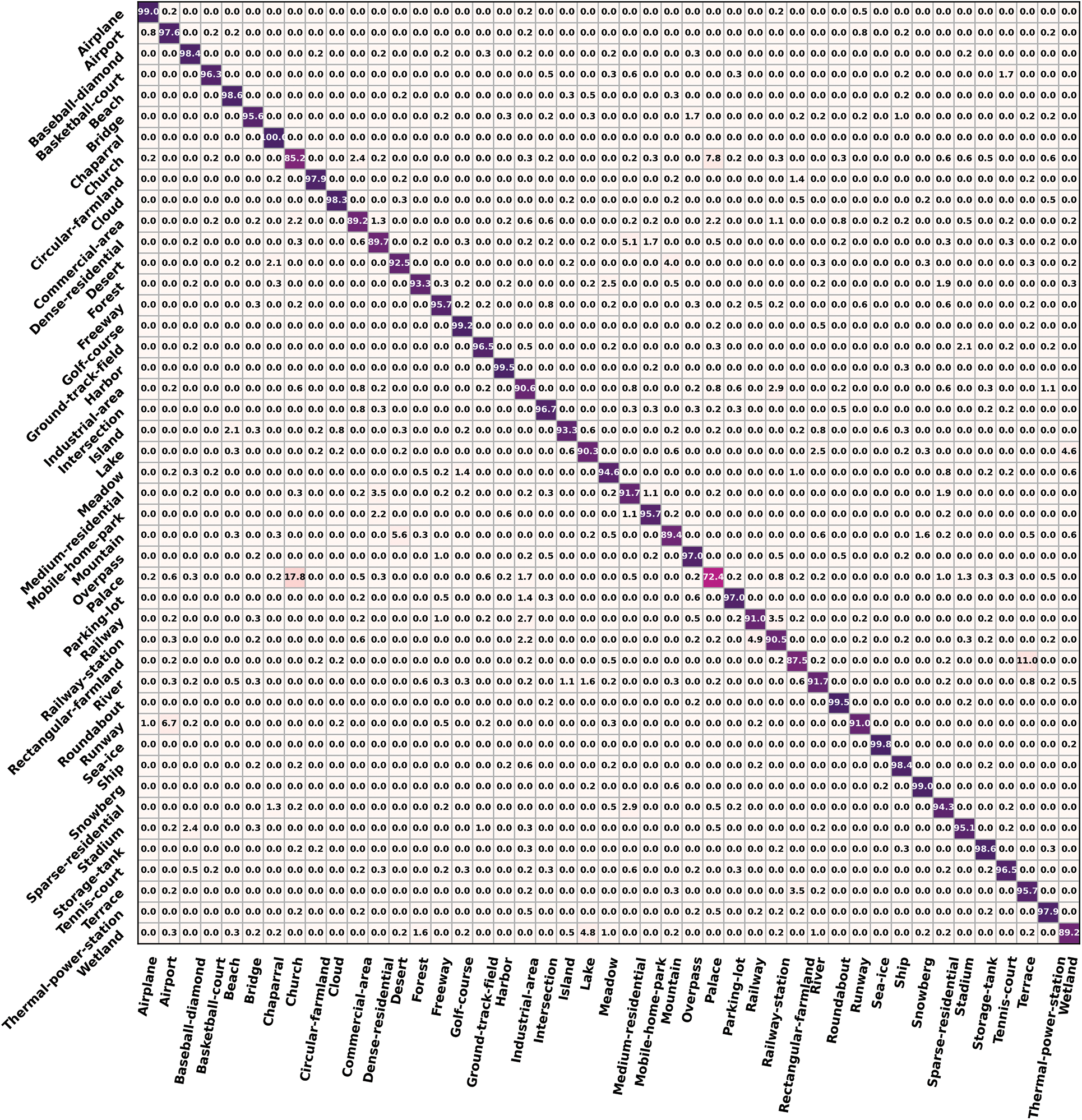
Figure 6: Confusion matrixes of NWPU45D at 10% training ratios

The confusion matrixes of NWPU45D at 20% training ratios are shown in Fig. 7. There are 27 subclasses with an OA above 95.7%. Confusion is most prevalent in the church and palace, which have an OA of less than 90%. Similarly, the OA results of six subclasses, including the commercial area, dense residential area, mountain, palace, rectangular farmland, and wetland, have increased by 3%–13% when compared to the results of the 10% training ratio. However, the OA result for the church has only increased by 1%. It reveals that the covariate shift in the Church subclass is more significant.

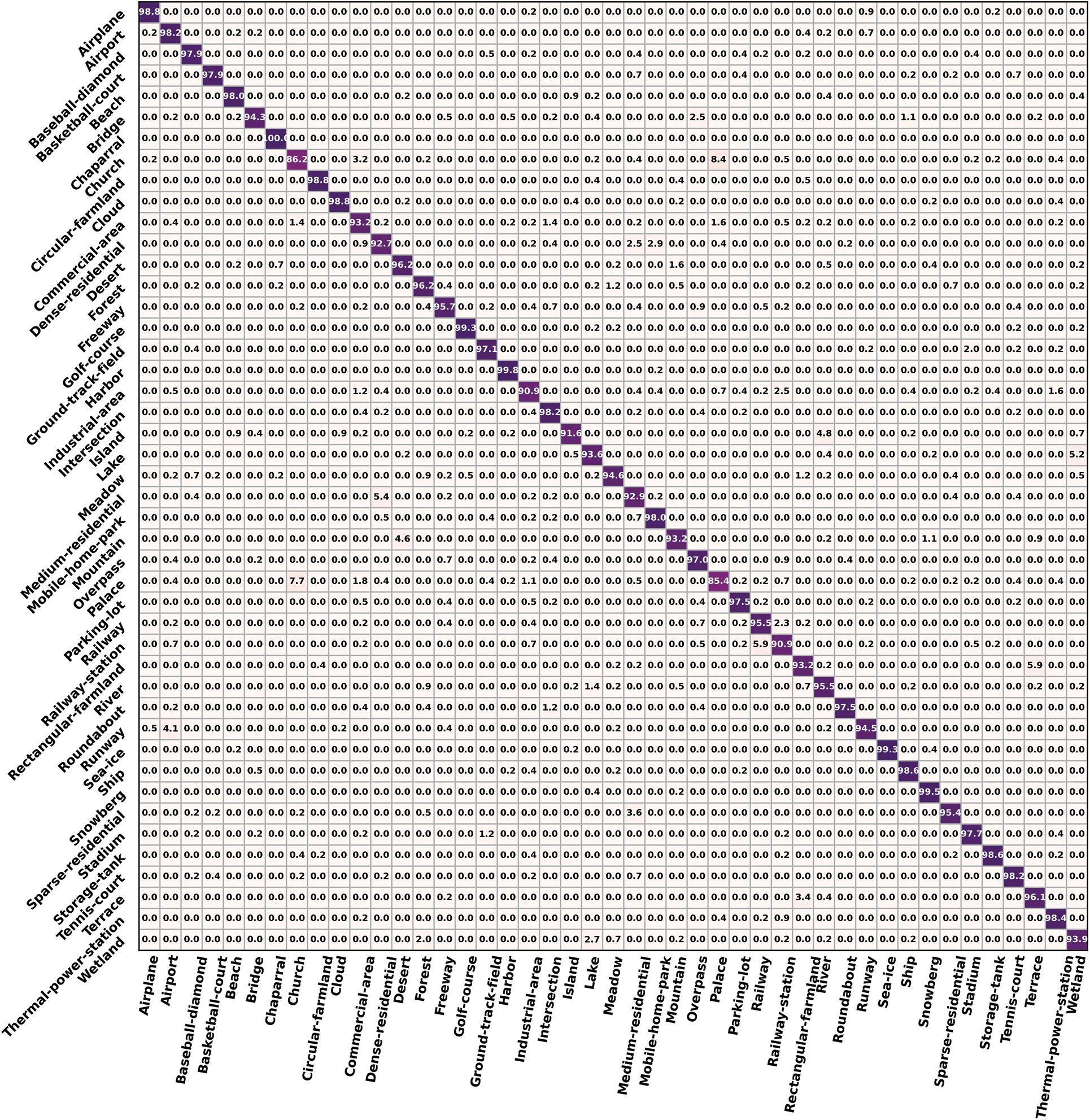
Figure 7: Confusion matrixes of NWPU45D at 20% training ratios

In brief, the confusion results of FST-EfficientNetV2 are consistent with its predecessor and other prior studies. More importantly, the OA and confusion results of FST-EfficientNetV2 on the two benchmark datasets have shown a greatly improved performance over the other prior methods. Meanwhile, with fewer training samples, the FST-EfficientNetV2 improves more significantly. It implies better representational ability.

5  Discussions

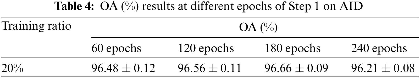
DA is now widely employed in DL-based methods for RSI-SC tasks. However, the problems of distribution shift arising from the indispensable technique of DL have seldom been investigated before the author’s work. More crucially, the author’s work only scratches the surface of dilemmas that have long existed in prior works. The OA results at different epochs in the interval of 60 to 240 of Step 1 on AID are shown in Table 4. The results show that the total iteration steps on the RSC-transformed images are not increasing in size. A significant over-fitting arises as the training epochs increase in Step 1. In other words, it will result in suboptimal performance if the training optimization is absent and not quantified.

To the best of the author’s knowledge, these problems of distribution shift introduced by data augmentation have not been noticed in the previous DL-based works for RSI-SC to date. These issues may result in a suboptimal or unfair outcome for the previous methods.

Nevertheless, there are still some limitations in our study. Firstly, the author’s work has not been tested in the other STOA CNN architecture, and the aforementioned problems have not been proven yet. Secondly, the spatial attention mechanism has not been involved in the base model of FST-EfficientNetV2. It means an optimal successor only with some low-cost modification.

6  Conclusions

The interpretation of RSI has been a labor-intensive task owing to the explosion of on-board sensors in the past two decades. Hence, the automatic techniques for RSI’s interpretation are becoming more crucial than ever. The DL-based methods, particularly the CNN methods, have played a key role to date. However, too many CNN methods employ complex, incomprehensible, and costly strategies to achieve better accuracy for RSI-SC. In fact, it is unnecessary.

To address this problem, the author proposes a novel and efficient method named FST-EfficientNetV2. The algorithm employs a routine transfer learning strategy corresponding to fast training characteristics. Some crucial algorithmic tweaks and hyperparameter re-optimizations are updated. It achieves a noticeable increase in accuracy of 0.3%–1.1% over its predecessor. More importantly, GPU hardware costs are reduced by 75%–81%, with training time costs reduced by 60%–80%. It achieves an amazing performance with a 1.7%–6.2% increase in accuracy compared to the other former SOTA methods. More interestingly, the new algorithm only differs from its predecessor by a few algorithmic tweaks and hyper-parameter re-optimizations.

The results demonstrate that an efficient CNN method for RSI-SC can be achieved with simplicity and automation. On the other hand, this study also proves the importance of training optimization strategies for RSI-SC. More crucially, the distribution shift introduced by DA techniques has been proven to be vital to the method’s performance for RSI-SC. In other words, the data distribution shift may cause previous studies to be incorrect to some extent.

In addition, the FST-EfficientNetV2 ideals may have good generality in different CNN architectures for achieving optimal performance for RSI-SC. We will investigate all similar questions in the future.

Acknowledgement: Thanks to the anonymous reviewers for their valuable suggestions.

Funding Statement: Hunan University of Arts and Science provided doctoral research funding for this study (grant number 16BSQD23). Fund of Geography Subject ([2022] 351) also provided funding.

Conflicts of Interest: The author declares that he has no conflicts of interest to report regarding the present study.

References

1. X. Sun, B. Wang, Z. Wang, H. Li, H. Li et al., “Research progress on few-shot learning for remote sensing image interpretation,” IEEE Journal of Selected Topics in Applied Earth Observations and Remote Sensing, vol. 14, pp. 2387–2403, 2021. [Google Scholar]
2. M. Sheykhmousa, M. Mahdianpari, H. Ghanbari, P. Ghamisi and S. Homayouni, “Support vector machine versus random forest for remote sensing image classification: A meta-analysis and systematic review,” IEEE Journal of Selected Topics in Applied Earth Observations and Remote Sensing, vol. 13, pp. 6308–6325, 2020. [Google Scholar]
3. X. X. Zhu, D. Tuia, L. Mou, G. S. Xia, L. Zhang et al., “Deep learning in remote sensing: A comprehensive review and list of resources,” IEEE Geoscience & Remote Sensing Magazine, vol. 5, no. 4, pp. 8–36, 2018. [Google Scholar]
4. P. Wange, B. Bayram and E. Sertel, “A comprehensive review on deep learning based remote sensing image super-resolution methods,” Earth-Science Reviews, vol. 232, no. 15, pp. 104110, 2022. [Google Scholar]
5. M. Ye, L. Ji, L. Tianye, L. Sihan, Z. Tong et al., “A lightweight model of VGG-U-Net for remote sensing image classification,” Computers, Materials & Continua, vol. 73, no. 3, pp. 6195–6205, 2022. [Google Scholar]
6. N. Ruiwen, M. Ye, L. Ji, Z. Tong, L. Tianye et al., “Segmentation of remote sensing images based on U-Net multi-task learning,” Computers, Materials & Continua, vol. 73, no. 2, pp. 3263–3274, 2022. [Google Scholar]
7. T. Liu, P. Liu, X. Jia, S. Chen, Y. Ma et al., “Sea-land segmentation of remote sensing images based on SDW-UNet,” Computer Systems Science and Engineering, vol. 45, no. 2, pp. 1033–1045, 2023. [Google Scholar]
8. Z. Zakria, J. Deng, R. Kumar, M. S. Khokhar, J. Cai et al., “Multiscale and direction target detecting in remote sensing images via modified YOLO-v4,” IEEE Journal of Selected Topics in Applied Earth Observations and Remote Sensing, vol. 15, pp. 1039–1048, 2022. [Google Scholar]
9. T. Manh Tuan, T. Thi Ngan and N. Tu Trung, “Object detection in remote sensing images using picture fuzzy clustering and mapreduce,” Computer Systems Science and Engineering, vol. 43, no. 3, pp. 1241–1253, 2022. [Google Scholar]
10. A. Shafique, G. Cao, Z. Khan, M. Asad and M. Aslam, “Deep learning-based change detection in remote sensing images: A review,” Remote Sensing, vol. 14, no. 4, pp. 871, 2022. [Google Scholar]
11. G. Cheng, X. Xie, J. Han, L. Guo and G. S. Xia, “Remote sensing image scene classification meets deep learning: Challenges, methods, benchmarks, and opportunities,” IEEE Journal of Selected Topics in Applied Earth Observations and Remote Sensing, vol. 13, pp. 3735–3756, 2020. [Google Scholar]
12. S. Chaib, H. Liu, Y. Gu and H. Yao, “Deep feature fusion for VHR remote sensing scene classification,” IEEE Transactions on Geoscience and Remote Sensing, vol. 55, no. 8, pp. 4775–4784, 2017. [Google Scholar]
13. G. Cheng, Z. Li, X. Yao, L. Guo and Z. Wei, “Remote sensing image scene classification using bag of convolutional features,” IEEE Geoscience and Remote Sensing Letters, vol. 14, no. 10, pp. 1735–1739, 2017. [Google Scholar]
14. Q. Wang, S. Liu, J. Chanussot and X. Li, “Scene classification with recurrent attention of VHR remote sensing images,” IEEE Transactions on Geoscience and Remote Sensing, vol. 57, no. 2, pp. 1155–1167, 2018. [Google Scholar]
15. H. Song, “A more efficient approach for remote sensing image classification,” Computers, Materials & Continua, vol. 74, no. 3, pp. 5741–5756, 2023. [Google Scholar]
16. M. Tan and Q. V. Le, “EfficientNetV2: Smaller models and faster training,” 2021. [Online]. Available: https://arxiv.org/abs/2104.00298v3 [Google Scholar]
17. Y. Liu, Y. Liu and L. Ding, “Scene classification by coupling convolutional neural networks with Wasserstein distance,” IEEE Geoscience and Remote Sensing Letters, vol. 16, no. 5, pp. 722–726, 2018. [Google Scholar]
18. Y. Liu, C. Y. Suen, Y. Liu and L. Ding, “Scene classification using hierarchical Wasserstein CNN,” IEEE Transactions on Geoscience and Remote Sensing, vol. 57, no. 5, pp. 2494–2509, 2018. [Google Scholar]
19. Q. Zhu, Y. Zhong, L. Zhang and D. Li, “Adaptive deep sparse semantic modeling framework for high spatial resolution image scene classification,” IEEE Transactions on Geoscience and Remote Sensing, vol. 56, no. 10, pp. 6180–6195, 2018. [Google Scholar]
20. W. Zhang, P. Tang and L. Zhao, “Remote sensing image scene classification using CNN-CapsNet,” Remote Sensing, vol. 11, no. 5, pp. 494, 2019. [Google Scholar]
21. Y. Liu, Y. Zhong and Q. Qin, “Scene classification based on multiscale convolutional neural network,” IEEE Transactions on Geoscience and Remote Sensing, vol. 56, no. 12, pp. 7109–7121, 2018. [Google Scholar]
22. R. Zhu, L. Yan, N. Mo and Y. Liu, “Attention-based deep feature fusion for the scene classification of high-resolution remote sensing images,” Remote Sensing, vol. 11, no. 17, pp. 1996, 2019. [Google Scholar]
23. R. Minetto, M. P. Segundo and S. Sarkar, “Hydra: An ensemble of convolutional neural networks for geospatial land classification,” IEEE Transactions on Geoscience and Remote Sensing, vol. 57, no. 9, pp. 6530–6541, 2019. [Google Scholar]
24. S. Amin, B. Alouffi, M. I. Uddin and W. Alosaimi, “Optimizing convolutional neural networks with transfer learning for making classification report in COVID-19 chest X-rays scans,” Scientific Programming, vol. 2022, pp. 13, 2022. [Google Scholar]
25. J. Howard, “Training imagenet in 3 hours for 25 minutes,” 2018. [Online]. Available: https://www.fast.ai/2018/04/30/dawnbench-fastai/ [Google Scholar]
26. E. Hoffer, B. Weinstein, I. Hubara, T. Ben-Nun and T. Hoefler, “Mix & match: training convnets with mixed image sizes for improved accuracy, speed and scale resiliency,” 2019. [Online]. Available: https://arxiv.org/abs/1908.08986 [Google Scholar]
27. H. Touvron, A. Vedaldi, M. Douze and H. Jégou, “Fixing the train-test resolution discrepancy,” 2020. [Online]. Available: https://arxiv.org/abs/2003.08237v1 [Google Scholar]
28. Z. Liu, H. Mao, C. Y. Wu, C. Feichtenhofer, T. Darrell et al., “A ConvNet for the 2020s,” in Proc. CVPR, New Orleans, LA, USA, pp. 11976–11986, 2022. [Google Scholar]
29. I. Loshchilov and F. Hutter, “Decoupled weight decay regularization,” 2019. [Online]. Available: https://arxiv.org/abs/1711.05101 [Google Scholar]
30. C. Szegedy, V. Vanhoucke, S. Ioffe, J. Shlens and Z. Wojna, “Rethinking the inception architecture for computer vision,” 2015. [Online]. Available: https://arxiv.org/abs/1512.00567 [Google Scholar]
31. M. Sandler, A. Howard, M. Zhu, A. Zhmoginov and L. C. Chen, “MobileNetV2: Inverted residuals and linear bottlenecks,” in Proc. CVPRW, Salt Lake City, UT, USA, pp. 4510–4520, 2018. [Google Scholar]
32. S. Gupta and B. Akin, “Accelerator-aware neural network design using AutoML,” 2020. [Online]. Available: https://arxiv.org/abs/2003.02838 [Google Scholar]
33. J. Hu, L. Shen and G. Sun, “Squeeze-and-excitation networks,” in Proc. CVPR, Salt Lake City, UT, USA, pp. 7132–7141, 2018. [Google Scholar]
34. G. S. Xia, J. Hu, F. Hu, B. Shi, X. Bai et al., “AID: A benchmark data set for performance evaluation of aerial scene classification,” IEEE Transactions on Geoscience and Remote Sensing, vol. 55, no. 7, pp. 3965–3981, 2017. [Google Scholar]
35. G. Cheng, J. Han and X. Lu, “Remote sensing image scene classification: Benchmark and state of the art,” Proceedings of the IEEE, vol. 105, no. 10, pp. 1865–1883, 2017. [Google Scholar]
Cite This Article
Copyright © 2023 The Author(s). Published by Tech Science Press.
This work is licensed under a Creative Commons Attribution 4.0 International License , which permits unrestricted use, distribution, and reproduction in any medium, provided the original work is properly cited.
Downloads
Citation Tools