Improving the Transmission Efficiency of a WSN with the IACO Algorithm

1  Introduction

With the development of sensor technology and wireless communication technology, as a self-organizing wireless sensor network (wireless sensor network, WSN) has been more and more applied [1,2]. The wireless sensor network can sense and collect various pieces of environmental information on the coverage area in real time, using multi-hop routing to aggregate and transmit data. Wireless sensor networks have technical advantages such as rapid deployment, self-organization, strong concealment, and high fault tolerance. It can obtain information without being restricted by the environment. To comprehensively monitor the network deployment environment, the wireless sensor network is generally densely populated with wireless nodes. In addition, it is necessary to collect data regularly and frequently and send it to neighbor nodes, which not only results in highly redundant data being transmitted across the network but also increases the energy consumption burden of nodes, affecting the working time and usage of wireless sensing networks. Therefore, aggregating wireless transmissions in wireless sensor networks, reducing node energy consumption, and increasing the WSN’s working time have become the focus of WSN’s research [3–5].

In this paper, we use the Improved Ant Colony Algorithm (IACO) to perform many practical research objectives, such as optimal path finding for wireless sensor networks and optimal path calculation for real traffic. Fig. 1 is an application diagram of data fusion transmission in wireless sensor networks. In wireless sensor networks, the IACO be proposed it can prolong the network life cycle, realize optimal data fusion transmission, and identify the optimal network path. Compared with routing algorithms such as shortest path tree (SPT), ant colony optimization (ACO), and balanced clustering routing protocol (EBCRP), the IACO has many advantages. For example, it (1) shows strong self-adjustment, (2) supports multi-path, (3) has local or global path optimization capability, and (4) is easy to integrate with other algorithms [6–8].

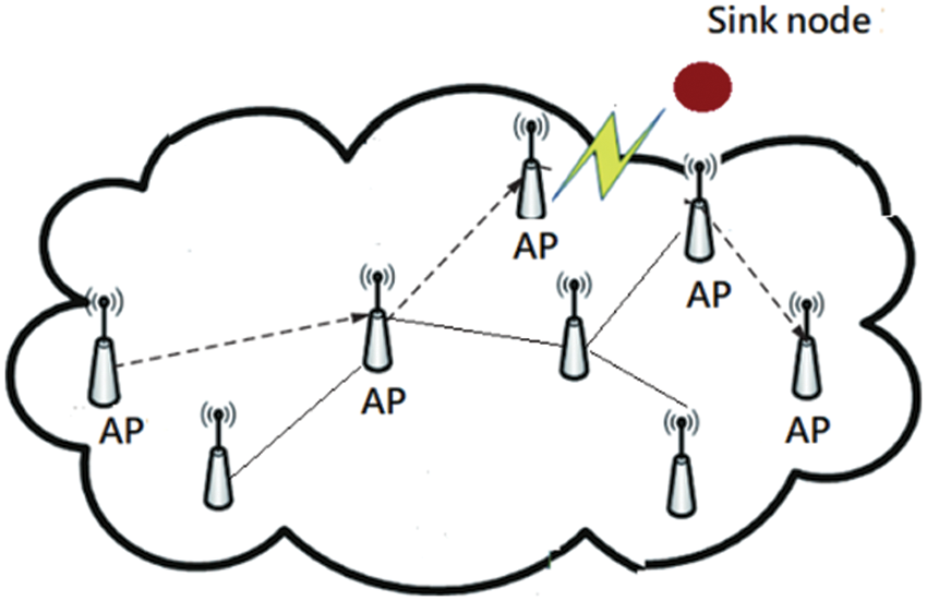
Figure 1: Schematic diagram of WSN data fusion transmission

The Marco Dorigo mentioned ant colony optimization algorithm in 1992. Its purpose is to find a probability algorithm for the optimal path in the network path graph. It is a simulated evolutionary algorithm. In some current research that the methods have many good features. The purpose of this study is to optimize and reform the design of WSN parameters, and compare it with other optimization algorithms. The experimental numerical results prove that the improved ant colony algorithm has rich application value, especially in wireless network related applications [9,10].

The point-to-ppoint network based on the WSN model is shown in Fig. 2. Each central node of WSN forms a point-to-point computing wireless network; its connotation includes multiple central nodes and general nodes; the task of these nodes is to collect, store and analyze data, and finally perform computing work. This invistigate adopts the ant colony algorithm work arrangement method, uses the data index to manage the network in the network norm server, and realizes the processing data, the data fusion and overall decision of each central node according to the just-in-time work schedule, and obtains the analysis results in the final step . This study adopts a point-to-point wireless ant colony network structure, which can reduce the communication burden and computing energy consumption, and is conducive to improving the transmission efficiency of wireless sensory networks [11,12].

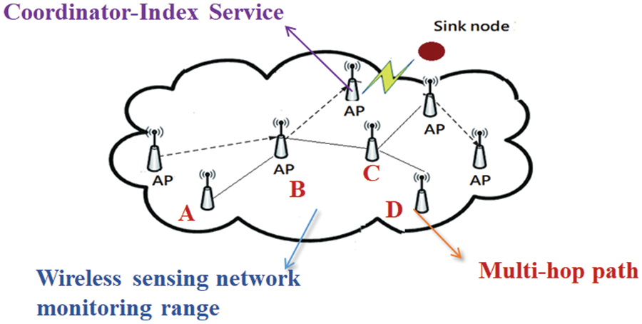
Figure 2: Peer-to-peer wireless sensing network structure

2  Literatures Survey

Ants are one of the most common and abundant insect species on earth, often visible in groups to humans. The group biological intelligence characteristics of these insects have attracted the attention of some scholars. When observing the foraging habits of ants, Italian scholars Dorigo, Maniezzo, and others found that ants can always find the shortest path between the food source and the nest. The study found that the ants in a group cooperate by communicating and coordinating through a volatile chemical called pheromone, which they leave on their path. Chemical communication is one of the basic information communication methods adopted by ants and plays an important role in the living habits of ants. The entire ant colony cooperates with each other through this information hormone, forming positive feedback, so that ants on multiple paths gradually gather on the shortest path [13–15].

The IACO method be put forward that the global optimization characteristics and fast solution mode; so many researches use it as its application. It has the characteristics of distributed search and optimization calculation, which can prevent faster convergence of the method, and it is ensure the accuracy of calculation through the transmission and accumulation of feedback information. After the improvement and development of researchers in related fields, an acceptable solution can be found in the early period of investigation steps. This study has proposed deeply extended and advanced during the experimental verification [16–18].

The ICAO method be used is robust in this research; a self-organizing parallel algorithm in which each ant's search process is independent of other ants and communicates only through pheromones. Ant colony algorithm is not only reliable but also has powerful global search ability. The number of parameters of the ant colony algorithm is small, and the setting is simple. It is easy to apply the ant colony algorithm to other combinatorial optimization problems. Another feature is that the requirements for the initial path are not high, and manual adjustment is required [19–23].

The ICAO method is mentioned has been successfully applied to combinatorial optimization problems, especially when the network assignment traffic is ever-changing and web nodes that links would be rejoin and fail informal. Another recent application of unmanned is aerial vehicles and ground communication vehicles for reconnaissance operations [24]. In the existing research, ant colony intelligence calculus has become the focus of today’s artificial intelligence research. Its practical use is the prospect of swarm intelligence application, because the foraging behavior of ant colony is parallel and distributed, which makes this algorithm especially suitable for parallel computing and processing [25,26]. The ant colony algorithm originated from solving the TSP problem, but the current applications all use swarm intelligence computing as its application field, that is, swarm strategy. For example, in exciter circuit design for huge System, coloring questions in graphics, maximum load equilibrium questions, and shipping adjustment questions and so on. Optimal path questions in WSN are all manifestations and applications of swarm intelligence computing. Therefore, the combination of parallel execution of ant colony algorithm and swarm computing in this study has great potential and contribution in resolving many composite application questions in WSN [27–29].

3  Methods of Assigning Tasks

In order to achieve the lower central node power squander and immediacy demand of WSN, this study proposes a method of assigning tasks to adjust the work, which aims to enhance the life cycle and task execution ability of the central node and cut down power squander. This investigates uses the sensors network all points and calculates some relation allocation method, which includes two evaluation factors such as network energy consumption and execution time [30].

3.1 Execution Time Evaluation Index

The wireless sensor network task execution time includes three parts: the transmission time Tsend, the access time Tvisit, the and processing time Tdeal−with. The data processing time Tdeal−with is affected by the computing capability and the amount of computation the central node needs to accomplish. The data transmission time Tsend is related to the amount of transmitted data Numsend and the wireless network bandwidth (Band−Width), as shown in Eq. (1).

Tsend=NumsendBand−Width(1)

Tvisit is the data access time, which depends on the number and size of data packets. Because data packets are read and written the same number of times, the data access times is approximately three times the read and write time. The relationship between the numbers of data visits, the data visit time Numvisit and the number of data Store is shown in Eq. (2).

Tvisit=3 NumvisitStore(2)

The data processing time Tseal−with varies by application. Fig. 3 shows the relationship between data processing time and system parameters. Generally, the existing experimental research shows that memory usage and CPU usage, especially in wireless sensing. The WSN systems have a relatively linear parallelism between the system-coefficient and the information fusion of all points. The all points have corresponding processing time in different states [31].

Figure 3: Work assignment relationship to system time parameters

In the point-to-point computing of WSN, each central point transmits data in parallel. So the execution time TImplement to complete all tasks is the maximum time taken by the central node to complete the task, as shown in Eq. (3).

TImplement=max0<i<n⁡((Tsend(i))Band−Width+2 NumvisitStore+Tdeal−with(i))(3)

Correspondingly, the relative execution time evaluation index of node ni is shown in Eq. (4).

eEI(ni)=TImplementTReference Time(4)

In Eq. (4), TReference Time is a predefined reference time.

3.2 Evaluation Index of Power Consumption in WSN

Evaluation index of energy consumption in WSN is similar to the execution time. It includes three parts: the processing energy consumption Edeal−with,the transmission energy consumption Esend, and the access energy consumption Evisit. The data processing energy consumption Edeal−with is related to the data processing time Tdeal−with and the central node processing power Pdeal−with, as shown in Eq. (5).

Edeal−with=Pdeal−withTdeal−with(5)

The data transmission energy consumption Esend is related to the data transmission time Tsend and the energy consumption power Pdeal−with of the wireless communication module. The data access energy consumption Evisit is determined by the data access time Tvisit and the central node processing power Pdeal−with. Therefore, the total energy consumption of the wireless sensor network is shown in Eq. (6) [31].

Etotal=∑i=1n⁡Tsend(i)Psend(i)+∑i=1n⁡(3Tvisit(i)+Tdeal−with(i))Pdeal−with(i)(6)

Since the energy consumption ratio of transmitting 2-bit data to processing 2-bit data is about 1000:1000000, in practical applications, the influence of processing and accessing energy consumption is usually ignored and only the communication energy consumption is discussed.

Given the minimum transmission energy consumption Psend(min) under the standard distance Wdistance(min), the central node instantly transmits the signal and the spatial distance Wp,q between Nodep and Nodeq is related as shown in Eq. (7) [32].

Pi,send=Wp,q2Wdistance(min)2×(4π)2θMfMcρ2×Psend(min)(7)

In Eq. (7), Mf is the transmission coefficient of the central node Nodep, Mc is the receiving coefficient of the central node Nodeq, ρ is the wireless communication wavelength, and θ is the system power consumption factor. Since (4π)2θMfMcρ2×Psend(min) is a constant, Wp,q2Wdistance(min)2 is used as the evaluation index of unit data transmission energy consumption. The life cycle of a wireless sensor network is Assigning Tasks, which is a very important indicator besides energy consumption. In this study, the life of the node that first exhausts energy is used to calculate the life of the network. Therefore, this study tries its best to use the method of uniform energy consumption of central nodes to prolong the survival time of the network. After completing the communication between node Nodep and node Nodeq, the remaining energy average of each node can be measured by energy entropy theory. In this study, the residual energy of the central node Nodecent at Time is set as Engerx and Eq. (8) is used to define the proportional relationship of the residual energy of the node Nodecent:

In this study, after completing the communication between node Nodeq and node Nodep, the mean of is left over power of each point can be obtained by measuring the energy entropy theory. There be left over power of the central point Nodecent at Time is set to Engerx and Eq. (8). It is used to define the proportional relationship of node Nodecent remaining energy:

I(Nodecent)=lg⁡(1p(Engerx))=−lg⁡(p(Engerx))(8)

In Eq. (8), p(Engerx) is the ratio of the residual energy of node Nodecent to the total residual energy of the network. According to the above formula, the average degree of residual energy of the entire network can be obtained as shown in Eq. (9).

In Eq. (8), p(Engerx) is the ratio of the remaining energy of node Nodecent divided by the total remaining energy of the network. According to Eq. (8), this research can get the average residual energy of the whole network as shown in Eq. (9).

H(l′)=−∑Engerx∈lIp(Engerx)lgp(Engerx)(9)

In Eq. (9), H(1′) is the entropy of the remaining energy of the entire wireless sensing network after the completion of data transmission at Time. The larger the entropy value, the more evenly distributed the remaining energy and the longer the corresponding network lifetime. Considering the unit residual energy entropy evaluation index and data transmission energy consumption evaluation index comprehensively, the network energy consumption evaluation index of node li is obtained as shown in Eq. (10) [33].

eEI(1i)=−Wp,q2Wdistance(min)2H(li′)(10)

3.3 Comprehensive Evaluation Index

In this study, the time-energy comprehensive evaluation index is used to achieve the influence of network energy consumption and balanced execution time on the optimal execution method of wireless sensor node assignment work, as shown in Eq. (11) [34].

ComeEI =γmax1<i<n(etime(ni))+(1−γ)∑i=1n⁡eEI (ni)(11)

In Eq. (11), γ is a correction parameter, and its purpose is to influence the power squander on the optimal working mode during the average work execution period. Because the number of node centers that can be allocated is adjusted with the scale of the WSN, the optimal work allocation method demands to adjust the diversification of the WSN instantly and dynamically. This research employed a IACO method to motorize the optimal work assignment method for wireless sensor networks [35–38]. The information hormone of the central node of the network determines the ability to find the shortest path and calculate the fast approach to stability of the IACO method. If the value of the α parameter is bigger, the central point data radius expansion operation is too fast, the method to collect is too early and it was not reach the best answer. Conversely, if the value of the α parameter is insignificant, the central point data radius expansion operation of the network will be slow, which will cause the entire system to converge too slowly. Consequently, this research mentioned to renew the data radius these central node of the optimal and suboptimal paths at the end of each cycle, and to calculate the shortest path. The flowchart of the algorithm proposed in this study is shown in Fig. 4 [39]. These shortest paths are calculated to form a shortest path tree of the wireless sensor network from the merge point to the origin point.

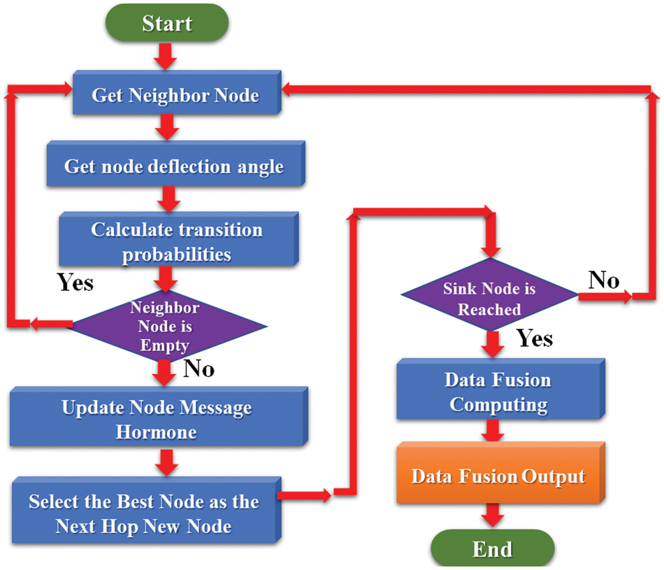
Figure 4: The information fusion method for flow chart model

4  Experimental Analysis and Discussion

4.1 Energy Efficiency Task Distribution Control

Under the hardware experiment framework of this research: (1) Use 35 network central nodes and complete the detailed multi-layer operation (seven layers) (2) The system places 150 central nodes for energy consumption measurement (3) Wireless sensor network The protocol is IEEE 802.11, and the central processing unit operating frequency is as high as 203MHz. The network record the operation period of the WSN, and the improved group WSN is employed to collect and train information, and the execution results are recorded. During the working procedure of the WSN, each central node measures its own residual energy in real time, and sends the result to the network index server for recording.

The experimental environment of this research is a typical wireless sensor network structure, with a total of 180 central nodes, which perform data calculation tasks of wireless sensor nodes. The web index server will use a modified ant colony algorithm energy-efficient work distribution method to complete the distribution work. In this study, the general genetic algorithm, the general ant colony algorithm, the multi-ant colony algorithm and the proposed improved ant colony algorithm are used for experiments. Fig. 5 is the analysis of data fusion transmission and energy consumption processing time in this experiment. From this experiment, it can be verified that the improved ant colony algorithm has the fastest convergence speed when dealing with multi-node optimization problems. When the number of iterations is 200, the optimal solution has been converged. This experiment analyzes the optimization of network energy efficiency and work allocation, and analyzes the trend of energy consumption and processing time as the number of network central nodes changes.

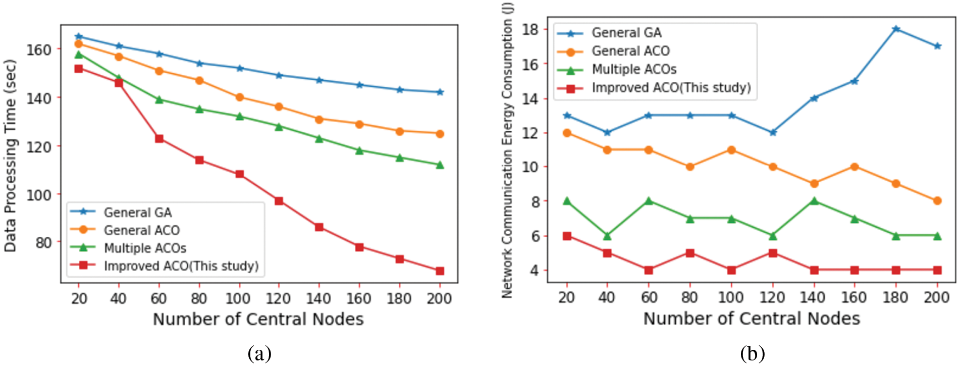
Figure 5: Simulation results of energy-efficient task scheduling methods: (a) information processing time and (b) wireless sensor network energy consumption

Fig. 5 shows that the information during the process of the center point’s node of the point-to-point network structure will be adjusted according to the number of central nodes, and the increase in the number of central nodes will increase the WSN power spender of the WSN. The information during the process and WSN power spender of the power-saving work arrange method using the IACO method are always higher than other algorithms. Generally speaking, if the information processing time of the single-center node wireless network structure is kept above 300 s, the communication energy consumption of the wireless sensor network varies between 4 and 9 J. The preliminary simulation results of this experiment show that the IACO method work arranges method are mentioned and helps to reasonably and effectively allocate the storage tasks in this study, information transport and deal with of every WSN node to the working status of the central node, and gradually Greatly improve network energy consumption and life cycle. The IACO varies with the parallel all points. Experiments prove that the IACO be mentioned has better stability and global optimization search ability. [40,41].

4.2 Packet Aggregation Delay Comparison

The hardware architecture of this experiment is as follows: (1) Randomly deploy 10–100 wireless sensor nodes (2) Construct a circular area (wireless sensor network) with a radius of 100 m. In order to verify the performance of various algorithms in this experiment, the single ACO algorithm, multiple ACO algorithm, general ant colony optimization (ACO) algorithm are compared with the method be mentioned in this research. According to the Python programming simulation test, adjust the parameter settings as shown in Table 1. After 50~68 simulation calculations in this experiment, it is concluded that different parameter combinations in the ACO will effect on time and efficiency of stabilization of optimal Network routing computation.

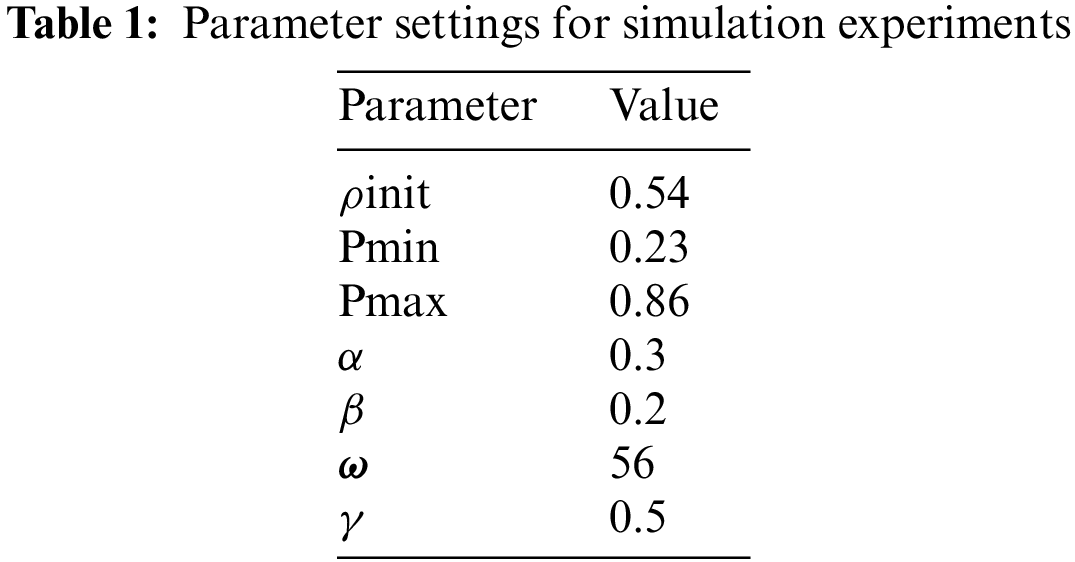
Fig. 6 compares the performance of the four algorithms in terms of packet aggregation latency in wireless sensor networks. As the number of nodes increases, the increase of wireless packet aggregation delay is close to linear. The delay performance of general ACO and single ACO algorithm is poor. A variety of ACO algorithms take into account the factor of data delay, and the delay effect is relatively good. The delay performance of the algorithm proposed in this experiment is the best. When the number of central nodes is greater than 130, the delay growth trend will slow down. This is because the algorithm proposed in this experiment combines the factors of load and distance when selecting the path and its biggest advantage is that it can independently select the optimal network transmission path.

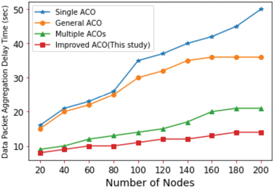
Figure 6: Comparison of data packet aggregation delays for four algorithms

4.3 Performance Evaluation Index

In this study, the algorithm’s performance is preliminarily evaluated in terms of three aspects: network life cycle, node load variance, and data collection delay [42].

4.3.1 Life Cycle of Wireless Sensor Network

Fig. 7 shows the life cycle of WSN under different number of nodes. The life cycle of the WSNs are the most appropriate execution parameters. The IACO be employed in this research takes the energy consumption of the central node as the basis of the reference network life cycle when constructing information fusion. This experiment only studies the energy consumption of the central node. From the statistics of the experiment, this The method proposed by me focuses on balancing the network load, and observes that the energy consumption of the central node is the lowest, so the network life cycle of the algorithm proposed in this research is better than other algorithms [43–45].

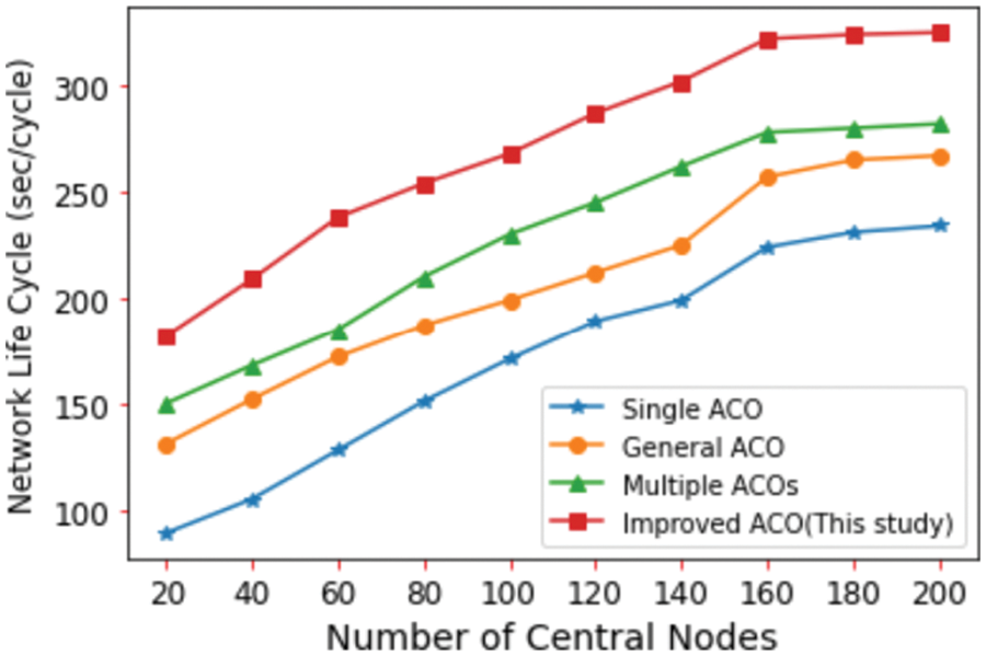
Figure 7: Life cycle of wireless sensor network

4.3.2 Central Node Load Variance

In this experiment, the central node load variance in the wireless sensor network is used as the measurement basis for load balancing, as shown in Eq. (12). Among them, L is the lave power spender of all WSN point, n is the center points, Li is the lave power of center point i, S2 is the maximum loader variance of center points. Fig. 8 shows the center point maximum loader variance.

S2=∑i=1n(Li−L¯)2n−1(12)

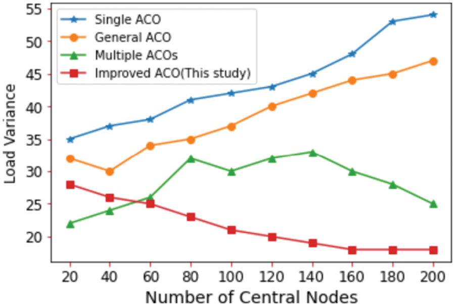
Figure 8: Central node load variance

Fig. 8 indicates that with an increase in time, the maximum point loader variance in the method proposed in this study gradually becomes smaller, which indicates that the threshold strategy is adopted in the data transmission stage, which balances the node energy of the network and prevents some nodes from consuming energy too quickly, dying prematurely, and reducing network performance. Since the multiple ACO algorithms constructs a data fusion tree with self-adjustment of energy and comprehensively considers the selection weight of energy in the next hop node, it also has a significant effect on the energy balance of the network. However, the single ACO and the general ACO algorithms do not fully consider the node energy, and the residual energy value between nodes is quite different, which is not conducive to extending the network life cycle and wastes a lot of energy.

4.3.3 Information Collection Latency

This experiment is to compare the efficiency of information collection delay. Data transmission latency is a serious parameter to observe the implement measurement of the method proposed in this research in terms of data fusion. Fig. 9 shows the change curves of the efficiency comparison of the information collection delay of the four methods. From the experimental results, it is found that the information collection delay with the increase or decrease of the network size. The method be employed in this research and the multiple ACO algorithms are more adequate in terms of information collection delay. They can get the best latency. However, other algorithms have longer delays in information collection and poorer responses.

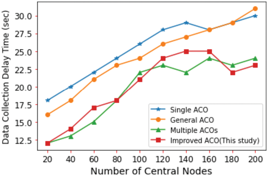
Figure 9: Information collection latency

5  Node Efficiency Regression Analysis and Supervised Learning

This study proposes an IACO method for information fusion in WSN. This algorithm can save the power spender of network central points and optimize to wireless transmission router and distance. The algorithm adjusts the selection probability of the central node when performing data fusion calculations, and updates information hormones for the best multiple paths at the same time. This study uses regression analysis to simulate and compare the life cycle, central node energy consumption and learning algorithm in this study. The proposed algorithm can effectively reduce node energy consumption, improve network load balance, prolong network life cycle, and effectively predict future node life cycle and learning status.

5.1 Node Efficiency Regression Analysis

In this section, the node energy is analyzed. Fig. 10a shows a schematic diagram of the node energy model of a concentric circle. The energy at the center point is the largest. Because of the relationship between the wireless environments, the electric energy is distributed into a gradient descent energy diagram as it goes to the periphery of the concentric circle. As a result, when distributing the locations of the nodes in the wireless sensing network, the energy distribution conditions must be considered. Fig. 10b shows a linear regression analysis diagram of the central node, in which each coordinate value of (xi,yj) represents the relationship between the life cycle and the energy of the central sensing node of the wireless sensing network. Fig. 10c displays a multiple regression analysis graph of the optimal solution. Because this graph is closer to the real graph of the relationship between the number of nodes and energy, the prediction from the model is also correct.

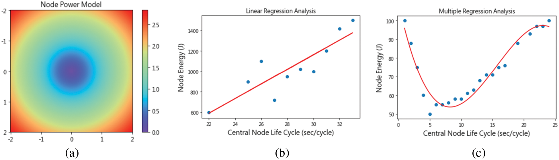
Figure 10: (a) Node energy model. (b) Linear regression analysis diagram of the central node.(c) Multiple regression analysis diagram of the optimal solution

In the previous references, we have repeated the concept of mean or median value. The core idea of using regression analysis here is to identify the best value for all distribution points such that the sum of the distances of the real values is zero, leading to an optimization result using the least squares method. In the data on the relationship between the life cycle and the energy of the real node, we compared the predicted data. The model in Figs. 10b, 10c provides use with an excellent ability to predict data and verify that the real data and the predicted data are the best match.

Regression analysis is widely used in wireless sensor network research. This study uses regression analysis to study the real and predicted relationship between node life cycle and energy. The authors use the coefficient of determination R2 as a criterion to judge whether the regression model is valid and its explanatory power is strong or weak, as shown in Eq. (13).

R2=∑(Y^−Y¯)2/∑(Y−Y^)2(13)

where (Y^−Y¯) represents the variation between the node energy fit value and the mean value, (Y−Y^) represents the variation between the node measurement value and the fit value, and the range of R2 is taken as [0,1]. An R2 value closer to 1 indicates that the life cycle of the node has a stronger ability to affect the energy of the node and the established regression model is more suitable. The R2 value in Fig. 10b is 0.72, while the R2 value in Fig. 10c is 0.86. Therefore, the Fig. 10c has a strong optimization performance.

5.2 Supervised Learning

In machine learning, we can divide the actual measurement data into training data and test data. Generally, 82% of the data is used for training and 18% of the data is used for testing. During the learning process, we can build a regression model from the training data and use the test data to judge whether the established regression model is good enough. In the previous discussion, we established a multiple regression model and also conducted research on numerical prediction. We then brought the test data into the regression model and compared the results to judge whether the regression model is capable of presenting and explaining all the existing states and prediction results.

Fig. 11a shows that the R2 value is 0.86, and the closer the coefficient of determination to 1, the more optimal is the regression model (a value greater than 0.5 usually indicates that the model has excellent ability to optimize). Fig. 11b verifies that the k-mean cluster analysis prediction of the regression model is accurate and applicable. Figs. 11a, 11b displays the prediction distribution maps of sensing nodes in space. In the figure, the X and Z axes are the relative positions of each node compared to the center node and the Y axis is the energy comparison value of each node and the center point. The three graphs in Figs. 12a–12c are used to compare the models for predicting the relationship between nodes and energy. The graph in Fig. 12a, at R2 = 0.93, is the best, and the graph in Fig. 12b is the second best. The predictive model in Fig. 12c has the weakest optimization ability.

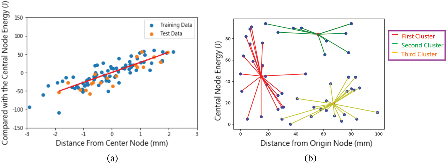
Figure 11: (a) Supervised learning and (b) cluster analysis

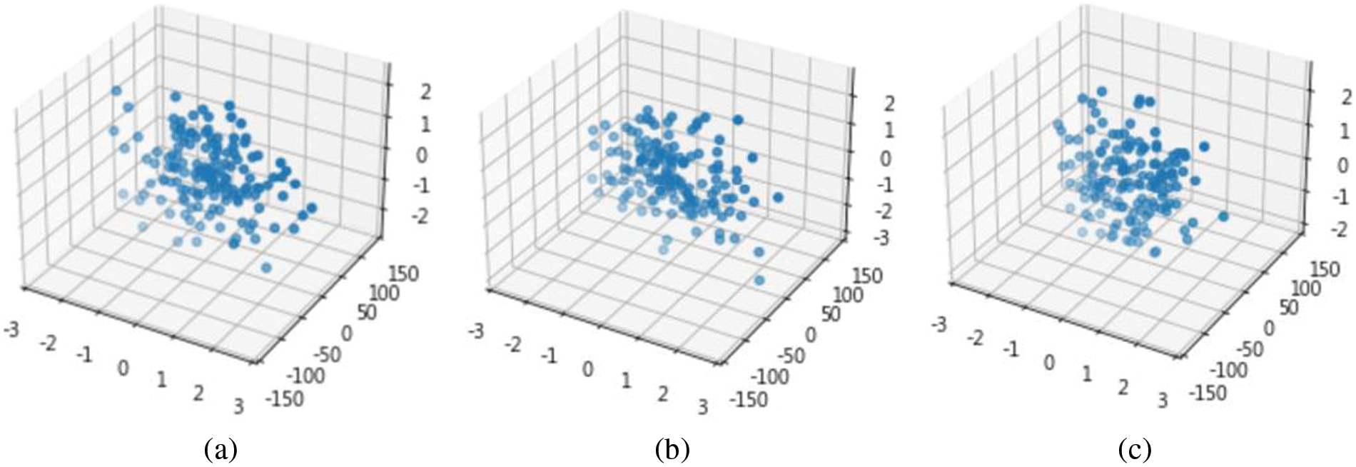
Figure 12: Prediction distribution maps of sensing nodes in space. (a) R2=0.68, (b) R2=0.84, and (c) R2=0.93

6  Conclusions and Future Works

An optimal design can reduce the cost of constructing a wireless sensor network. This research mentioned an IACO method, whose purpose is to combine the global parallel search ability and the calculation probability strategy of information fusion to solve the optimal transmission design problem of many different types WSN. The IACO method is an adjustment and integration stage in the calculation procedure. This system endows the algorithm with the ability to conduct a global search, and starts searching at multiple central nodes in the distribution area at the same time, and improves the reliability and accuracy of the algorithm. This study successfully proposed an improved ant colony algorithm, which has the advantages of a very robust sorting combination operator that can enhance the global search ability.

The IACO be employed in this research is suitable for providing methods for optimizing task assignment in wireless sensor networks. This method uses a probabilistic model to evaluate the network life cycle and energy consumption performance, takes increasing the effective network coverage as the optimization goal, searches the global network through the ant colony intelligent algorithm, and introduces the energy efficiency into the ant information radical evolution calculation. The method process of work distribution is accelerated, and finally the convergence speed of applying group algorithm to swarm intelligence calculation is accelerated. In summary, the IACO be employed in this research can be applied not only to any WSN-based IoT architecture, but also to high-performance information fusion computing and large-scale IoT with strict energy consumption requirements.

Acknowledgement: This research was supported by the Department of Electrical Engineering at National Chin-Yi University of Technology. The authors would like to thank the National Chin-Yi University of Technology, Takming University of Science and Technology, Taiwan, for supporting this research.

Funding Statement: The authors received no specific funding for this study.

Conflicts of Interest: The authors declare that they have no conflicts of interest to report regarding the present study.

References

1. Z. Wang, H. Ding, B. Li, L. Bao and Z. Yang, “An energy efficient routing protocol based on improved artificial bee colony algorithm for wireless sensor networks,” IEEE Access, vol. 8, pp. 133577–133596, 2020. [Google Scholar]

2. C. Tunca, S. Isik, M. Y. Donmez and C. Ersoy, “Distributed mobile sink routing for wireless sensor networks: A survey,” IEEE Communication Surveys & Tutorials, vol. 16, no. 2, pp. 877–897, 2014. [Google Scholar]

3. G. Sun, D. Qin, T. Lan and L. Ma, “Research on clustering routing protocol based on improved PSO in FANET,” IEEE Sensors Journal, vol. 21, no. 23, pp. 27168– 27185, 2021. [Google Scholar]

4. A. V. d. Silva and G. S. Pavani, “Tackling multiple byzantine failures in optical networks routed by means of ant colony optimization,” in Proc. 2019 21st Int. Conf. on Transparent Optical Networks (ICTON), Angers, France, pp. 1–4, 2019. [Google Scholar]

5. X. Liu, S. Li and M. Wang, “An ant colony based routing algorithm for wireless sensor network,” International Journal of Future Generation Communication and Networking, vol. 9, no. 6, pp. 75–86, 2016. [Google Scholar]

6. H. Zhou and W. Lei, “Anti-eavesdropping scheme on physical layer for full-duplex relay system based on SWIPT,” in Proc. 2017 Int. Conf. on Computer Technology, Electronics and Communication (ICCTEC), Dalian, China, pp. 1445–1449, 2017. [Google Scholar]

7. A. Haber, S. A. Nugroho, P. Torres and A. F. Taha, “Control node selection algorithm for nonlinear dynamic networks,” IEEE Control Systems Letters, vol. 5, no. 4, pp. 1195–1200, 2021. [Google Scholar]

8. W. M. Zhang and F. B. Liao, “Improved uneven clustering routing algorithm for wireless sensor networks,” Journal of Sensors and Actuators, vol. 28, no. 5, pp. 739–743, 2019. [Google Scholar]

9. J. Z. Li, H. T. Wang and A. Tao, “An energy balanced clustering routing protocol for WSN,” Journal of Sensors and Actuators, vol. 26, no. 3, pp. 396–401, 2018. [Google Scholar]

10. C. Konstantopoulos, E. Koutroulis, N. Mitianoudis and A. Bletsas, “Converting a plant to a battery and wireless sensor with scatter radio and ultra-low cost,” IEEE Transactions on Instrumentation and Measurement, vol. 65, no. 2, pp. 388–398, 2016. [Google Scholar]

11. S. N. Daskalakis, G. Goussetis, S. D. Assimonis, M. M. Tentzeris and A. Georgiadis, “A uW backscatter-morse-leaf sensor for low-power agricultural wireless sensor networks,” IEEE Sensors Journal, vol. 18, no. 19, pp. 7889–7898, 2018. [Google Scholar]

12. U. Baroudi, “Robot-assisted maintenance of wireless sensor networks using wireless energy transfer,” IEEE Sensors Journal, vol. 17, no. 14, pp. 4661–4671, 2017. [Google Scholar]

13. N. Harris, A. Cranny, M. Rivers, K. Smettem and E. G. Barrett-Lennard, “Application of distributed wireless chloride sensors to environmental monitoring: Initial results,” IEEE Transactions on Instrumentation and Measurement, vol. 65, no. 4, pp. 736–743, 2016. [Google Scholar]

14. L. Ascorti, S. Savazzi, G. Soatti, M. Nicoli, E. Sisinni et al., “A wireless cloud network platform for industrial process automation: Critical data publishing and distributed sensing,” IEEE Transactions on Instrumentation and Measurement, vol. 66, no. 4, pp. 592–603, 2017. [Google Scholar]

15. J. Zhu, H. Yu, Z. Lin, N. Liu, H. Sun et al., “Efficient actuator failure avoidance mobile charging for wireless sensor and actuator networks,” IEEE Access, vol. 7, pp. 104197–104209, 2019. [Google Scholar]

16. W. Liang, Z. Xu, W. Xu, J. Shi, G. Mao et al., “Approximation algorithms for charging reward maximization in rechargeable sensor networks via a mobile charger,” IEEE/ACM Transactions on Networking, vol. 25, no. 5, pp. 3161–3174, 2017. [Google Scholar]

17. D. Spirjakin, A. Baranov and S. Akbari, “Wearable wireless sensor system with RF remote activation for gas monitoring applications,” IEEE Sensors Journal, vol. 18, no. 7, pp. 2976–2982, 2018. [Google Scholar]

18. J. Chen, J. Klein, Y. Wu, S. Xing, R. Flammang et al., “A thermoelectric energy harvesting system for powering wireless sensors in nuclear power plants,” IEEE Transactions on Nuclear Science, vol. 63, no. 5, pp. 2738–2746, 2016. [Google Scholar]

19. L. Shu, M. Mukherjee, X. Xu, K. Wang and X. Wu, “A survey on gas leakage source detection and boundary tracking with wireless sensor networks,” IEEE Access, vol. 4, pp. 1700–1715, 2016. [Google Scholar]

20. P. Gil, A. Santos and A. Cardoso, “Dealing with outliers in wireless sensor networks: An oil refinery application,” IEEE Transactions on Control Systems Technology, vol. 22, no. 4, pp. 1589–1596, 2014. [Google Scholar]

21. A. Cammarano, C. Petrioli and D. Spenza, “Online energy harvesting prediction in environmentally powered wireless sensor networks,” IEEE Sensors Journal, vol. 16, no. 17, pp. 6793–6804, 2016. [Google Scholar]

22. F. Sangare, Y. Xiao, D. Niyato and Z. Han, “Mobile charging in wireless-powered sensor networks: Optimal scheduling and experimental implementation,” IEEE Transactions on Vehicular Technology, vol. 66, no. 8, pp. 7400–7410, 2017. [Google Scholar]

23. A. Afsharinejad, A. Davy, B. Jennings and C. Brennan, “Performance analysis of plant monitoring nanosensor networks at THz frequencies,” IEEE Internet of Things Journal, vol. 3, no. 1, pp. 59–69, 2016. [Google Scholar]

24. S. Cai and V. K. N. Lau, “Zero MAC latency sensor networking for cyber-physical systems,” IEEE Transactions on Signal Processing, vol. 66, no. 14, pp. 3814–3823, 2018. [Google Scholar]

25. Q. Han, P. Liu, H. Zhang and Z. Cai, “A wireless sensor network for monitoring environmental quality in the manufacturing industry,” IEEE Access, vol. 7, pp. 78108–78119, 2019. [Google Scholar]

26. L. Shu, M. Mukherjee, L. Hu, N. Bergmann and C. Zhu, “Geographic routing in duty-cycled industrial wireless sensor networks with radio irregularity,” IEEE Access, vol. 4, pp. 9043–9052, 2016. [Google Scholar]

27. N. Harun, R. Ahmad and N. Mohamed, “WSN application in LED plant factory using continuous lighting (CL) method,” in Proc. 2015 IEEE Conf. on Open Systems (ICOS), Bandar Melaka, Malaysia, pp.24–26, 2015. [Google Scholar]

28. D. W. Upton, R. P. Haigh, P. J. Mather, P. I. Lazaridis, K. K. Mistry et al., “Gated pipelined folding ADC-based low power sensor for large-scale radiometric partial discharge monitoring,” IEEE Sensors Journal, vol. 20, no. 14, pp. 7826–7836, 2020. [Google Scholar]

29. J. E. Shuda, A. J. Rix and M. J. Booysen, “Towards module-level performance and health monitoring of solar PV plants using LoRa wireless sensor networks,” in Proc. 2018 IEEE PES/IAS Power Africa,Cape Town, South Africa, pp. 28–29, 2018. [Google Scholar]

30. G. Deepika and P. Rajapirian, “Wireless sensor network in precision agriculture: A survey,” in Proc. 2016 Int. Conf. on Emerging Trends in Engineering, Technology and Science (ICETETS), Pudukkottai, India, pp. 24–26, 2016. [Google Scholar]

31. R. I. Gomaa, I. A. Shohdy, K. A. Sharshar, A. S. Al-Kabbani and H. F. Ragai, “Real-time radiological monitoring of nuclear facilities using ZigBee technology,” IEEE Sensors Journal, vol. 14, no. 11, pp. 4007–4013, 2014. [Google Scholar]

32. Z. Lin, W. Wang, H. Yin, S. Jiang, G. Jiao et al., “Design of monitoring system for rural drinking water source based on WSN,” in Proc. 2017 Int. Conf. on Computer Network, Electronic and Automation (ICCNEA), Xi’an, China, pp. 1195–1200, 2020. [Google Scholar]

33. A. M. Ezhilazhahi and P. T. V. Bhuvaneswari, “IoT enabled plant soil moisture monitoring using wireless sensor networks,” in Proc. 2017 Third Int. Conf. on Sensing, Signal Processing and Security (ICSSS), Chennai, India, pp. 4–5, 2017. [Google Scholar]

34. X. Meng, W. Cong, H. Liang and J. Li, “Design and implementation of Apple Orchard Monitoring System based on wireless sensor network,” in Proc. 2018 IEEE Int. Conf. on Mechatronics and Automation (ICMA), Changchun, China, pp. 5–8, 2018. [Google Scholar]

35. B. Sridhar, S. Sridhar and V. Nanchariah, “Design of novel wireless sensor network enabled IoT based smart health monitoring system for thicket of trees,” in Proc. 2020 Fourth Int. Conf. on Computing Methodologies and Communication (ICCMC), Erode, India, pp. 11–13, 2020. [Google Scholar]

36. M. E. Haque, K. Majumder and S. Uddin, “Potential measure to enhance lifespan of power plant monitoring system in era of IoT,” in Proc. 2019 IEEE Int. Conf. on Power, Electrical, and Electronics and Industrial Applications (PEEIACON), Dhaka, Bangladesh, pp. 99–103, 2019. [Google Scholar]

37. P. Sreelakshmi, C. Prabhavathi and K. Navyashree, “Design and implementation of an arm cortex M0+ based low power sensor node for an IoT based plant monitoring system,” in Proc. 2018 3rd IEEE Int. Conf. on Recent Trends in Electronics, Information & Communication Technology (RTEICT), Bangalore, India, pp. 468–473, 2018. [Google Scholar]

38. G. Bloom, G. Cena, I. C. Bertolotti, T. Hu, N. Navet et al., “Event notification in CAN-based sensor networks,” IEEE Transactions on Industrial Informatics, vol. 15, no. 10, pp. 5613–5625, 2019. [Google Scholar]

39. W. Al-Dabbagh and T. Chen, “Design considerations for wireless networked control systems,” IEEE Transactions on Industrial Electronics, vol. 63, no. 9, pp. 5547–5557, 2016. [Google Scholar]

40. E. T. Iorkyase, C. Tachtatzis, P. Lazaridis, I. A. Glover and R. C. Atkinson, “Low-complexity wireless sensor system for partial discharge localization,” IET Wireless Sensor Systems, vol. 9, no. 3, pp. 158–165, 2019. [Google Scholar]

41. X. R. Zhang, X. Chen, W. Sun and X. Z. He, “Vehicle re-identification model based on optimized DenseNet121 with joint loss,” Computers, Materials & Continua, vol. 67, no. 3, pp. 3933–3948, 2021. [Google Scholar]

42. X. R. Zhang, H. L. Wu, W. Sun, A. G. Song and S. K. Jha, “A fast and accurate vascular tissue simulation model based on point primitive method,” Intelligent Automation & Soft Computing, vol. 27, no. 3, pp. 873–889, 2021. [Google Scholar]

43. J. Liu, D. Yang, M. Lian and M. Li, “Research on intrusion detection based on particle swarm optimization in IoT,” IEEE Access, vol. 9, pp. 38254–38268, 2021. [Google Scholar]

44. W. Zhang, J. Wang, G. Han, S. Huang, Y. Feng et al., “A data set accuracy weighted random forest algorithm for IoT fault detection based on edge computing and blockchain,” IEEE Internet of Things Journal, vol. 8, no. 4, pp. 2354–2363, 2021. [Google Scholar]

45. J. C. Lin, J. M. Wu, P. Fournier, Y. Djenouri, C. Chen et al., “A sanitization approach to secure shared data in an IoT environment,” IEEE Access, vol. 7, pp. 25359– 25368, 2019. [Google Scholar]