Improved Metaheuristics with Deep Learning Enabled Movie Review Sentiment Analysis

1  Introduction

The intersection of Artificial Intelligence (AI), linguistics and computer science is referred to as Natural Language Processing (NLP). Computers are mainly used to ‘understand’ or process the natural language to execute several manual tasks, namely, answering questions or translating the language. With the increased penetration of chat-bots and voice interfaces, the NLP technique has become the most significant contribution to the fourth industrial revolution. It is already a popular region of the AI domain. Various helpful applications have been developed in the domain of NLP. Exploiting a user’s information is a key to several applications in surveys conducted by associations, political campaigning processes etc., [1]. In addition, it is crucial for governments to understand public thoughts since it describes human activities and the ways to influence the opinions of others in a community. Various recommender mechanisms are prevalently used, whereas ‘personalization’ has become a norm for almost all services and products. In such cases, the inference of user sentiments is highly helpful in decision-making processes without clear feedback from the users [2]. Machine Learning (ML) techniques are used to achieve this objective, which depends on the similarities of the results [3]. The data required for conducting the Sentiment Analysis (SA) can be retrieved from online mass media in which the users generate huge volumes of data on a daily basis. These kinds of data sources are handled with the help of big data techniques. When using these techniques, the problems should be multi-faceted so that effective processing, data storage and access can be achieved to assure the dependability of the acquired outcomes [4]. The execution of automatic SA is an increasingly-investigated research subject. Though SA is a significant domain and results in an extensive array of applications, it cannot be executed as a single direct task and experiences several difficulties concerning NLP [5].

The sentiment Analysis technique is applied to automatically categorize the huge volumes of text as either positive or negative. With the explosive development of mass media, companies and organizations started employing big data procedures to process online data and achieve proactive decision-making and product development [6]. Recently, blogs, mass media and other social media platforms have drastically influenced people’s ordinary lives, especially how individuals express their thoughts. The derivation of valuable data, i.e., individuals’ opinions regarding a company’s brands, from a vast quantity of unstructured data becomes significant for many organizations and companies [7]. The SA technique’s application is confined to movie or product reviews and other areas like sports, news, politics and so on. For instance, the SA technique is employed to identify an individual’s opinions about a political party in online political disputes [8]. The SA technique is applied at the sentence as well as document levels. The document-level SA is utilized to classify the sentiments expressed in a file as either negative or positive. In the case of sentence-level SA, the sentiments exhibited in a sentence are investigated [9]. In the execution of SA, two techniques are broadly utilized such as the Lexicon-based technique, which employs the lexicons (i.e., a dictionary of words and its respective polarities) to assign the polarity; and the ML technique, which demands a huge volume of labelled datasets with manual annotation [10]. Recently, a deep ML-related automated feature engineering and classification process has been employed to outperform the existing manual feature engineering-related shallow classification approaches.

In literature [11], the researchers explored several NLP techniques to conduct sentiment analysis. The researchers categorized two distinct datasets such as the first one with multi-class labels and the other one with binary labels. In the case of binary classifiers, the authors used skip-gram word2vec and bag-of-words methods along with several classifiers such as Random Forest (RF), Logistic Regression (LR) and Support Vector Machine (SVM). In the case of multi-class classifier, they applied a Recursive Neural Tensor Network (RNTN). Pouransari et al. [12] introduced a new, context-aware, Deep Learning (DL)-driven Persian SA technique. To be specific, the suggested DL-driven automated feature-engineering technique categorized the Persian movie reviews as negative and positive sentiments. In this study, two DL techniques, the Convolutional Neural Network (CNN) and the Long-Short-Term Memory (LSTM), were used. A comparison was made with the results of the manual feature engineering-driven SVM-related technique.

Dashtipour et al. [13] presented an enhanced SA classification technique with the help of DL methods and achieved comparable outcomes from different DL techniques. This study used the Multilayer Perceptron (MLP) model as a reference point for other network outcomes. The authors used Long Short-Term Memory (LSTM), Recurrent Neural Network and CNN along with a hybrid method of CNN and LSTM methods for comparison purposes. These methods were comparatively evaluated using a dataset with 50 K movies’ review documents. In the study conducted earlier [14], heterogeneous features like Lexicon-based features, ML-related methods and supervised learning methods such as the Naïve Bayes (NB) method and the Linear SVM (LSVM) approach were employed to develop the model. The experimental analysis outcomes inferred that the application of the suggested hybrid technique, along with its heterogeneous features achieved a precise SA system compared to other baseline systems.

In literature [15], the authors identified and assigned a meaning to each and every word tweeted so far. In this study, the word2vec method, the CNN method and the LSTM method were combined so that the features can comply with stop words and tweet words. These methods were able to identify the paradigm of stop-word counts using its dynamic strategies. Gandhi et al. [16] recommended a hybrid method combining CNN and LSTM approaches in the name of Hybrid CNN-LSTM algorithm to overcome the SA issue. Initially, the authors employed Word to Vector (Word2Vc) technique to train the primary word embeddings. The Word2Vc technique converted the text strings as numerical value vectors and calculated the distances amongst the words. Then, they created sets of similar words based on their meanings. Then, the embedding procedure was executed in which the suggested method integrated the features derived by global max-pooling and convolution layers with long-term dependencies. The presented method also employed the dropout technologies, a rectified linear unit and a normalization procedure to enhance the precision.

The current study introduces an effective model named Improved Metaheuristics with Deep Learning Enabled Sentiment Analysis for Movie Reviews (IMDLSA-MR). The presented IMDLSA-MR technique initially applies different levels of pre-processing to convert the input data into a compatible format. Besides, the TF-IDF model is exploited to generate the word vectors from the pre-processed data. To analyse and classify the sentiments, the Deep Belief Network (DBN) model is utilized. Finally, the improved Jellyfish Search Optimization (IJSO) technique is employed for optimal fine-tuning of the hyperparameters related to the DBN model. In order to evaluate the better performance of the proposed IMDLSA-MR model, numerous experimental analyses were conducted.

2  Background Information: Problem Statement

The aim of the current study is to define the sentimental tendencies, expressed in a review sentence, at the aspect level. A user expresses a negative or positive sentiment towards the aspect terms such as ‘soup’ and the ‘pizza’. But, two dissimilar sentiments are attained for the aspect category ‘food’ since the aspect category includes different foods, and a reviewer holds completely distinct feelings about the categories. The current study focuses only on recognising the sentiments that can be expressed on the aspect category or a term in a review sentence.

Consider X=[xx⋯xn] refers to a review sentence that contains n words, xi represents the embedding vector mapped from the ith word. A={a,  a,  ⋯,  at}(1≤t<n) denotes a set of aspect concepts that is implicitly or explicitly involved in X. Especially, the aspect concept is an aspect category or an aspect term as the presented method is relevant. Here, L={l1,  l2,  ⋯,  lk} denotes a set of the pre-determined sentiment labels, lai∈L denotes the true labels of the aspect concept ai and l^ai∈L represents the predictive label of ai. Next, the aim of the study is to maximize the subsequent probability of each forecasted sentimental label of aspect concept in the provided X review sentence and model variable, θ .

∑i=1t⁡logP(l^=lai|X,  A,  θ) (1)

In Eq. (1), P represents the conditional probability of l^ai=lai for X, A and θ. Generally, the sentiment analysis tasks are performed on a review set instead of a review sentence. Here, S={X1,  X2,  ⋯,  Xm} denotes a set of review sentences, Xj indicates the jth sentence in S. Aj stands for a set of aspect concepts from Xj , laij∈L and l^aij∈L indicate the true and predictive labels of ai in Xj review sentence as described below.

∑j=1m⁡∑i=1t⁡logP(l^aij=laij|Xj,  Aj,  θ) (2)

3  Materials and Methods

In this work, a novel IMDLSA-MR methodology has been developed to analyse the sentiments in a movie reviews dataset. The presented IMDLSA-MR technique encompasses different stages such as classification, data pre-processing, feature extraction and parameter optimization. At the initial stage, the presented IMDLSA-MR technique applies different levels of pre-processing to convert the input data into a compatible format. Next, the TF-IDF model is exploited to generate the word vectors from the pre-processed data. Finally, the IJSO and the DBN model are applied to analyse and classify the sentiments. Fig. 1 illustrates the overall process of the IMDLSA-MR algorithm.

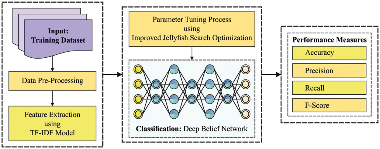
Figure 1: Overall process of IMDLSA-MR approach

3.1 Stage I: Data Cleaning and Pre-Processing

At the initial stage, the data pre-processing is performed at different levels, as briefed herewith.

•   In general, the text dataset contains words with dissimilar letter cases. The words with different cases are considered a challenge since it increases the vocabulary issues and subsequently result in complications. Hence, it is vital to modify the entire text to lower-case to prevent this issue.

•   The presence of punctuation marks in the text increases the complications due to which it is eliminated from the data set.

•   The numerical data present in the text is a problem for the proposed model’s components since it increases the vocabulary for the extracted text.

•   Specifies first and the last order: The word tokens such as the ‘<start>’ and the ‘<end>’ correspond to the first and the last of each sentence to represent the first and the final word of the forecasted order to the component.

•   Tokenization: The clean text is divided into constituent words whereas the dictionary containing the whole vocabulary such as index-to-word and word-to-index equivalent is obtained.

•   Vectorization: To resolve the issue of diverse lengths of sentences, short sentences are padded to the length of the long sentences.

Next, the TF-IDF model is exploited for the generation of the word vectors from the pre-processed data.

3.2 Stage II: DBN-Based Sentiment Classification

In this study, the DBN method is applied to analyse and classify the sentiments. Even though the Back Propagation (BP) approach is a highly-effective learning method with different layers of non-linear features, it is complex in nature. This characteristic improves the weight of the deep network that contains multiple layers of hidden units. This deep network demands a labelled training dataset that is challenging to develop [17]. The DBN method overcomes the limitations of the BP approach through unsupervised learning method. This is done to generate a layer of the feature detector, which in turn develops the statistical model of the input dataset without using any data from the essential output. A high-level feature detector captures complex high-order statistical models from the input dataset, which are later utilized in the prediction of the labels. The DBN method is an important tool for deep learning and was created from Restricted Boltzmann Machine (RBM). RBM has an effective training process that makes it suitable as the building block of the DBN approach.

RBM is a probabilistic graphical model that is considered a stochastic neural network in which the likelihood distribution is learnt over their input sets. RBM is a kind of Boltzmann machine with a constraint that its neurons should form a bipartite graph. A bipartite graph is a type of graph with a vertex (V) that is separated into two independent sets such as V1 (visible unit) and V2 (hidden unit). Each edge of the graph connects one vertex from V1 to V2 . Both sets might have symmetric connections between themselves, whereas it has no links amongst other nodes within a similar group.

A conventional RBM accepts the binary values for a hidden and a visible unit. This kind of RBM is termed as Bernoulli-Bernoulli RBM with a discrete distribution and two probable results that are labelled as n=0 and n=1 . When n=1 , it implies that the true values occur with P probability and if n=0 , it implies that the false cases occur with a probability q=1−p if 0<p<1.

RBM is an energy-related mechanism composed of n and m visible and hidden units, respectively. The vectors v and h represent the states of the visible and hidden units correspondingly and are determined as given below.

E(v, h)=−∑i=1n⁡aivi−∑j=1m⁡bjhj−∑i=1jn⁡∑=1m⁡viWijhj, (3)

In Eq. (3), vj refers to the state of the i - th visible unit, and hj indicates the state of the j - th hidden unit. Wij denotes the connection weight of the visible and the hidden units. Along with that, the bias weight (offsets) aj exists only for the visible units and bj for the hidden unit.

Once the variable is described, then the joint likelihood distribution of (v,  h) is found in terms of the energy function given below.

P(v, h)=1Ze−E(v,h)  (4)

Z=∑v,h⁡e−E(v,h), (5)

In this expression, Z refers to a normalized constant. Once the states of the visible unit are provided, the activation state of every hidden unit becomes conditionally independent. Thus, the activation probability of the jth hidden unit is given herewith.

P(hj=1|v)=σ(bj+∑ivi⁡Wij), (6)

Here, σ(x)=1/(1+e(−x)) represents a logistics’ sigmoid activation function. Likewise, assume a hidden state, h while the activation state of every visible unit is conditionally-independent and the probability of the i - th visible unit of v is given. Here, h can be attained as follows.

P(vi=1|h)=σ(ai+∑jhj⁡Wij). (7)

Differentiate a log-likelihood of the trainable dataset w.r.t W as given below.

∂logp(v)∂Wii=⟨vihj⟩daia−⟨vihj⟩model′  (8)

In Eq. (8), ⟨.⟩daia and⟨.⟩model indicates the predictable values of a dataset or a distribution model. The learning rule for the weight of a network in log probability-related trainable dataset is attained through the following equation.

ΔWij=e(⟨vihj⟩daia−⟨vihj⟩model) ′  (9)

In Eq. (9), e represents the learning rate. Since there is no direct connection in the hidden state of the RBM model, unbiased samples of ⟨vihj⟩daia can be acquired. Unfortunately, it is challenging to calculate the unbiased instance of ⟨vihj⟩model because it needs exponential duration. To prevent these problems, Contrastive Divergence (CD), a fast learning mechanism is used. The CD mechanism sets the visible variable as a trainable dataset. Next, the binary state of the hidden unit is calculated. When the state is selected for the hidden unit, ‘ reconstruction ’ is generated by setting every vi to 1 with a probability. Furthermore, the weight is attuned for every trainable pass.

ΔWii=e(⟨vihj⟩daia−vihj⟩recon) .  (10)

⟨vihj⟩data denotes the average value over each input dataset for every update, and ⟨vihj⟩recon indicates the average value; it can be assumed as a better calculation to ⟨vjhj⟩model.

The DBN model is a neural network that was created by stacking multiple layers of the RBM model. With the help of the stacked RBM, it is easy to develop a high-level description for the input dataset. The DBN model was developed as a conventional Artificial Neural Network (ANN) technique. In this model, the network topology was constructed using a layer of neuron models but with in-depth architecture and highly-sophisticated learning mechanics. However, a comprehensive human intelligence-based biological phenomenon was not modelled in this approach. The DBN training process has two stages: (1) fine-tuning and (2) greedy layer-wise pre-training. Here, the layer-by-layer pre-training includes the training of the module and its parameters in a layer-wise fashion using CD technique and an unsupervised training model. Initially, the training begins with a low-level RBM that receives the input from DBN method. The training is continued until the RBM reaches the top layer with DBN output. As a result, the learned features or the output of the preceding layer can be utilized as an input for the following RBM layers.

3.3 Stage III: IJSO Based Parameter Optimization

Finally, the IJSO algorithm is utilized for optimal fine-tuning of the hyperparameters related to the DBN method. The JSO technique was inspired from jellyfish behaviour in the ocean [18]. When finding their food, the jellyfishes exhibit the following behaviour. It follows the ocean movement or current inside the swarm and follows a time control method to switch between the movements. The authors witnessed numerous chaotic maps and a typical random method to find the best initialization method. This is to ensure that the method distributes the solution precisely within the searching region of the problem, which in turn fastens the convergence and avoids the solution from getting trapped in local minima issues. Based on the observations, it can be inferred that the JSO algorithm performs well in the logistic map, which is mathematically defined herewith.

X→i+1=ηX→i(1−Xi),  0≤X→0≤1  (11)

X→i+1 represents a vector that has the logistic chaotic value of the ith jellyfish. X→ denotes a primary vector of the jellyfish 0 that is randomly produced between 0 and 1. This vector is the starting point and helps in the development of logistic chaotic values for the remainder of the jellyfishes. The η is allocated with a value of 4. After initialization, all the solutions are noted whereas the one with an optimal fitness value is preferred as the position with the maximum food, X→∗. Next, the existing position of every jellyfish is upgraded to the ocean current or motion inside the swarm, according to the time control model, so the jellyfishes can switch between the movements. The ocean current is mathematically expressed below.

X→i(t+1)=X→i(t)+r→. ∗(X→∗−β∗r1∗μ)  (12)

In Eq. (12), r→ denotes a vector that is randomly produced within 0 and 1 and ∗ indicates the component-wise vector multiplication. β>0 signifies the distribution coefficient, which depends on the sensitivity analysis outcomes, i.e., β=3 . μ indicates the mean population and r1 represents a random value that lies between 0 and 1.

The movements inside the jellyfish swarm are separated into two motions such as active and passive. In passive movement, the jellyfish moves nearby the location and the novel position is shown below.

X→(t+1)=X→i(t)+r3∗γ∗(Ub−Lb)  (13)

In Eq. (13), r3 denotes a random value in the range of 0 and 1, and γ>0 represents the length of the motion nearby the existing position. Ub and Lb denote the upper and the lower bounds of the searching space, correspondingly. The active motion is arithmetically expressed as follows.

X→i(t+1)=X→i(t)+r→∗D→  (14)

In Eq. (14), r→ denotes a vector that comprises random values between 0 and 1. D→ is utilized to determine the direction of the motion of existing jellyfishes with the upcoming generation, and this motion often lies in the direction of optimal food position, as expressed below.

D→={X→(t)−X→j(t), if f(X→)<f(X→)X→(t)−X→i(t), otherwise (15)

In Eq. (15), j represents the index of the randomly-chosen jellyfish and f represents the fitness function. The time control model is utilized for switching amongst the ocean current, active and passive motions, and it involves a constant c0 as expressed mathematically below.

c(t)=(1−tt max )∗(2∗r−1)  (16)

In Eq. (16), t stands for the existing evaluation, tmax  denotes the maximal evaluation, and r represents a random value that lies between 0 and 1. Fig. 2 depicts the flowchart of the JSO technique.

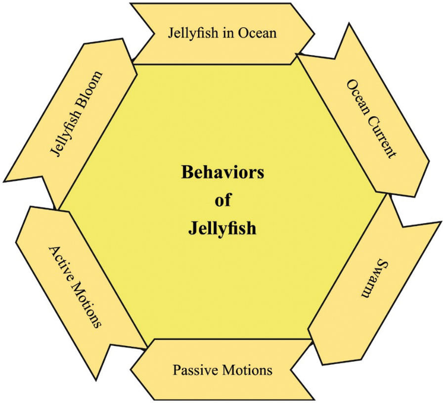
Figure 2: Flowchart of the JSO technique

The IJSO algorithm is derived using the Levy flight concept with JSO algorithm. The French mathematician Paul Levy proposed the concept of Levy flight in the 1930s [19]. It was a probability distribution with a random step size that follows the Levy distribution. Further, it can be a walking mode that transforms between the occasional long-distance searches and a large number of short-distance searches. Usually, the Mantegna algorithm is utilized for simulation processes, as expressed below.

u∼N(0,  δu2)  (17)

v∼N(0,  δv2)  (18)

δu={Γ(1+β)sin⁡(πβ2)Γ((1+β)2β×2(β−1)2)}1β  (19)

δv=1  (20)

Levy=δu×u|v|1β  (21)

Xi,jt+1={ Xbestt+Levy.|Xi,jt−Xbestt, if fi >fgXi,jt+K.(| Xi,jt−Xworstt |(fi−fw)+ε), if fj=fg (22)

In these expressions, u and v refer to the random numbers of the regular distribution, Levy can step-size the random values of the Levy distribution and β denotes a constant which is generally 1.5 [20]. The Levy flight random number is presented to the JSO algorithm, which makes it easier to get rid of the local optima issue. This in turn, enhances the optimization performance of the technique, the local exploration capability and the population diversity.

The IJSO method derives a FF to obtain enhanced classification outcomes. It determines a positive integer to indicate the superior outcomes of the candidate solution. In this article, classification error rate reduction is regarded as a FF and is presented in Eq. (23). The optimal solution has a minimum error rate, whereas the poor solution has a maximum error rate.

fitness(xi)=ClassifierErrorRate(xi)=number of misclassified samplesTotal number of samples∗100  (23)

4  Performance Validation

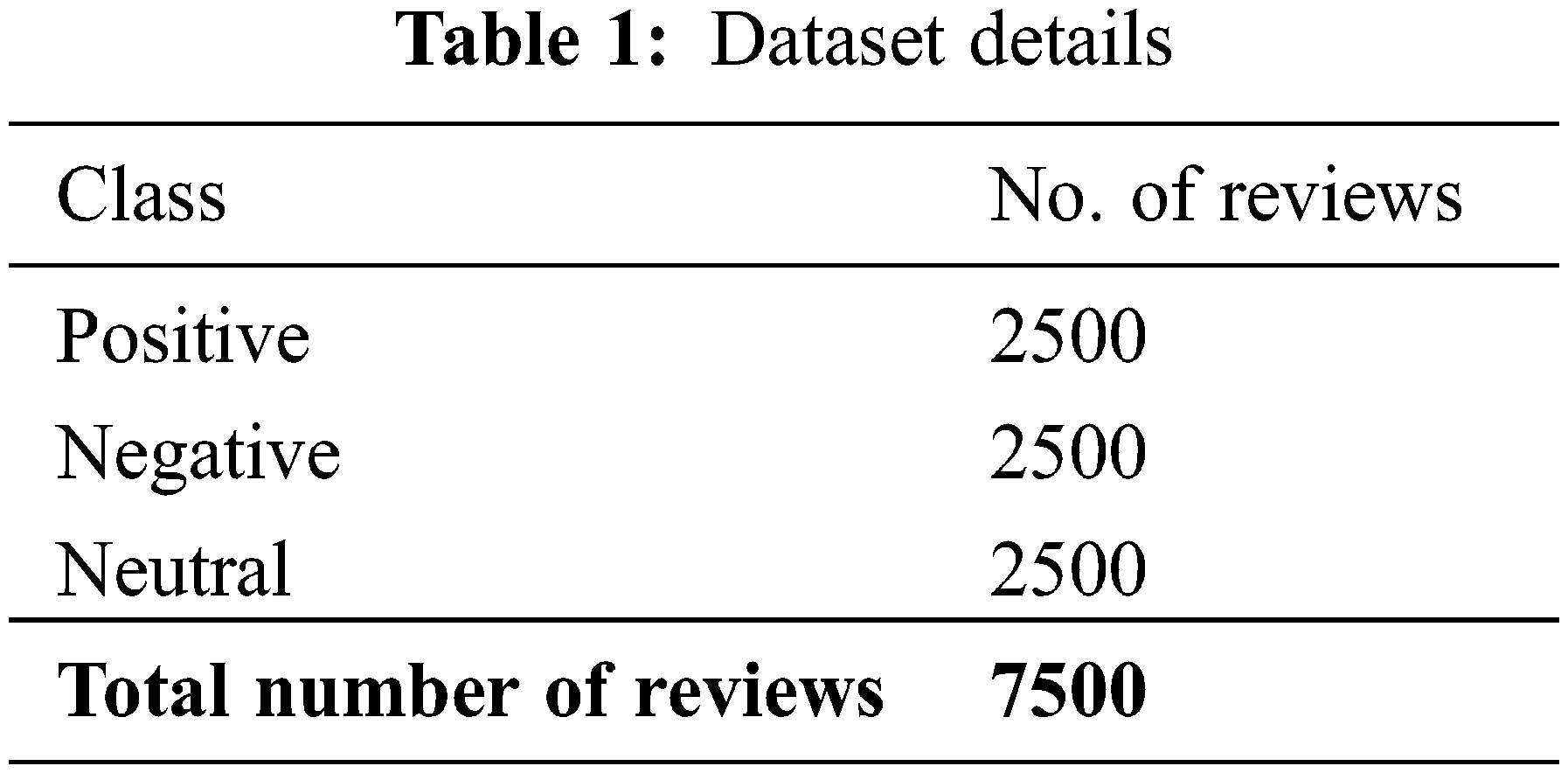
This section investigates the performance of the proposed IMDLSA-MR method using a dataset containing 7,500 movie reviews under three class labels, namely, positive, negative and neutral, with each label containing 2,500 reviews. The details of the dataset are given in Table 1.

The confusion matrices generated by the IMDLSA-MR model on the test data are shown in Fig. 3. On epoch 200, the proposed IMDLSA-MR model identified 2,402 samples as positive class, 2,481 samples as negative class and 2,419 samples as neutral class. Also, on epoch 600, the IMDLSA-MR method classified 2,442 samples under positive class, 2,485 samples under negative class and 2,452 samples under neutral class. In addition, on epoch 800, the proposed IMDLSA-MR technique categorized 2,427 samples under positive class, 2,481 samples under negative class and 2,425 samples under neutral class. Moreover, on epoch 1200, the IMDLSA-MR approach identified 2,414 samples as positive class, 2,457 samples as negative class and 2,331 samples as neutral class.

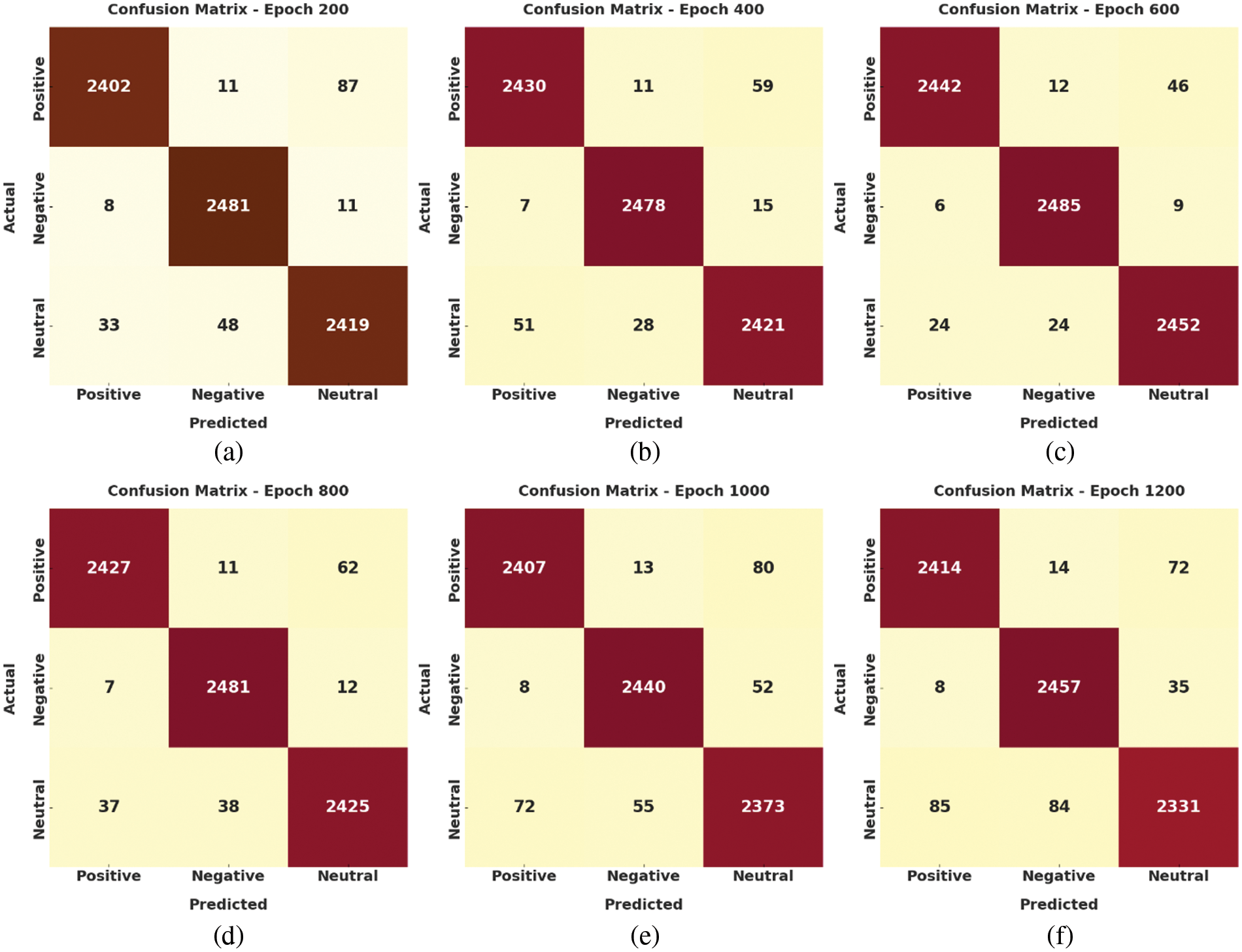
Figure 3: Confusion matrices of the IMDLSA-MR approach (a) Epoch 200, (b) Epoch 400, (c) Epoch 600, (d) Epoch 800, (e) Epoch 1000, and (f) Epoch 1200

Table 2 and Fig. 4 exhibit the classification outcomes of the proposed IMDLSA-MR model under a distinct number of epochs. The experimental values confirmed that the proposed IMDLSA-MR model gained effectual outcomes under every epoch count.

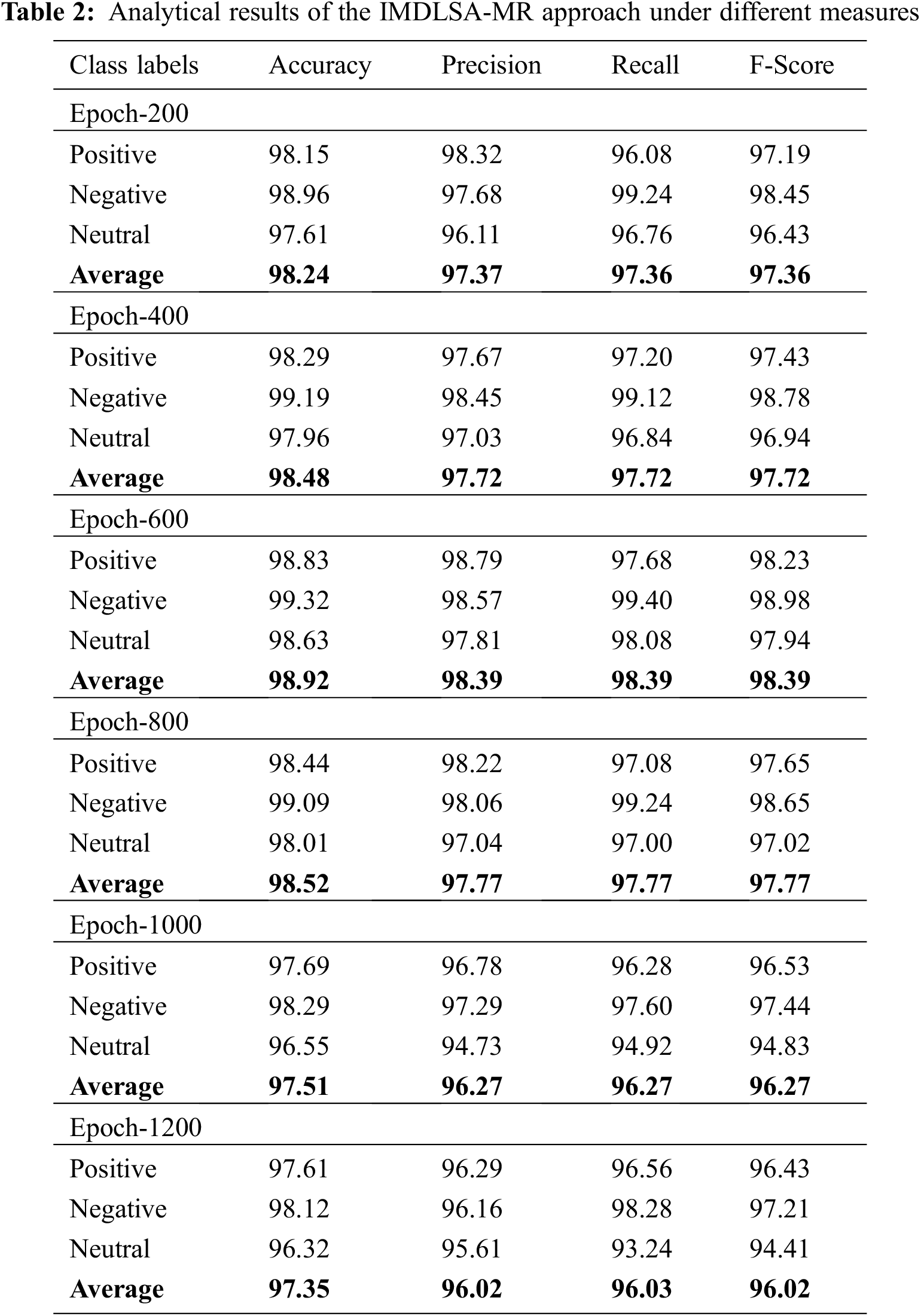
Figure 4: Analytical results of the IMDLSA-MR approach (a) Epoch 200, (b) Epoch 400, (c) Epoch 600, (d) Epoch 800, (e) Epoch 1000, and (f) Epoch 1200

For instance, on epoch 200, the IMDLSA-MR model produced an average accuy of 98.24%, precn of 97.37%, recal of 97.36% and an Fscore of 97.36%. Moreover, on epoch 600, the IMDLSA-MR methodology attained an average accuy of 98.92%, precn of 98.39%, recal of 98.39% and an Fscore of 98.39%. Furthermore, on epoch 800, the proposed IMDLSA-MR algorithm produced an average accuy of 98.52%, precn of 97.77%, recal of 97.77% and an Fscore of 97.77%. At last, on epoch 1200, the IMDLSA-MR approach accomplished an average accuy of 97.35%, precn of 96.02%, recal of 96.03% and an Fscore of 96.02%.

Both Training Accuracy (TA) and Validation Accuracy (VA) values, attained by the IMDLSA-MR method on the test dataset, are illustrated in Fig. 5. The experimental outcomes represent that the proposed IMDLSA-MR method reached the maximal TA and VA values whereas the VA values were higher than the TA values.

Figure 5: TA and VA analyses results of the IMDLSA-MR methodology

Both Training Loss (TL) and Validation Loss (VL) values, reached by the proposed IMDLSA-MR approach on the test dataset, are established in Fig. 6. The experimental outcomes imply that the proposed IMDLSA-MR methodology accomplished the least TL and VL values whereas the VL values were lower than the TL values.

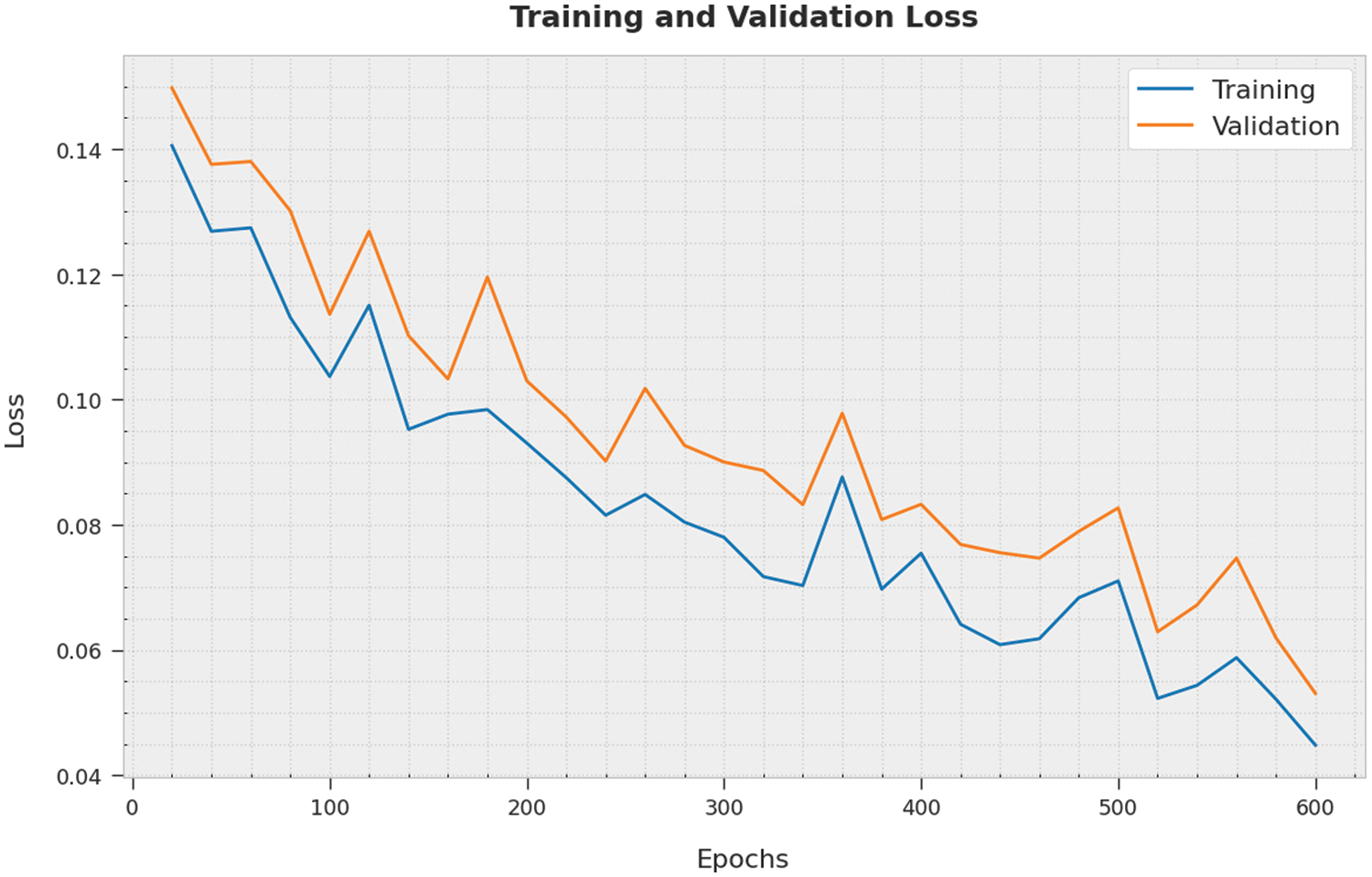
Figure 6: TL and VL analyses results of the IMDLSA-MR methodology

A clear precision-recall analysis was conducted on the IMDLSA-MR algorithm using the test dataset and the results are depicted in Fig. 7. The figure shows that the IMDLSA-MR technique produced enhanced precision-recall values under all the classes.

Figure 7: Precision-recall curve analysis results of the IMDLSA-MR methodology

A brief Receiver Operating Characteristic (ROC) curve analysis was conducted on the IMDLSA-MR approach using the test dataset, and the results are portrayed in Fig. 8. The results indicate that the proposed IMDLSA-MR method established its ability to categorize the test dataset under distinct class labels.

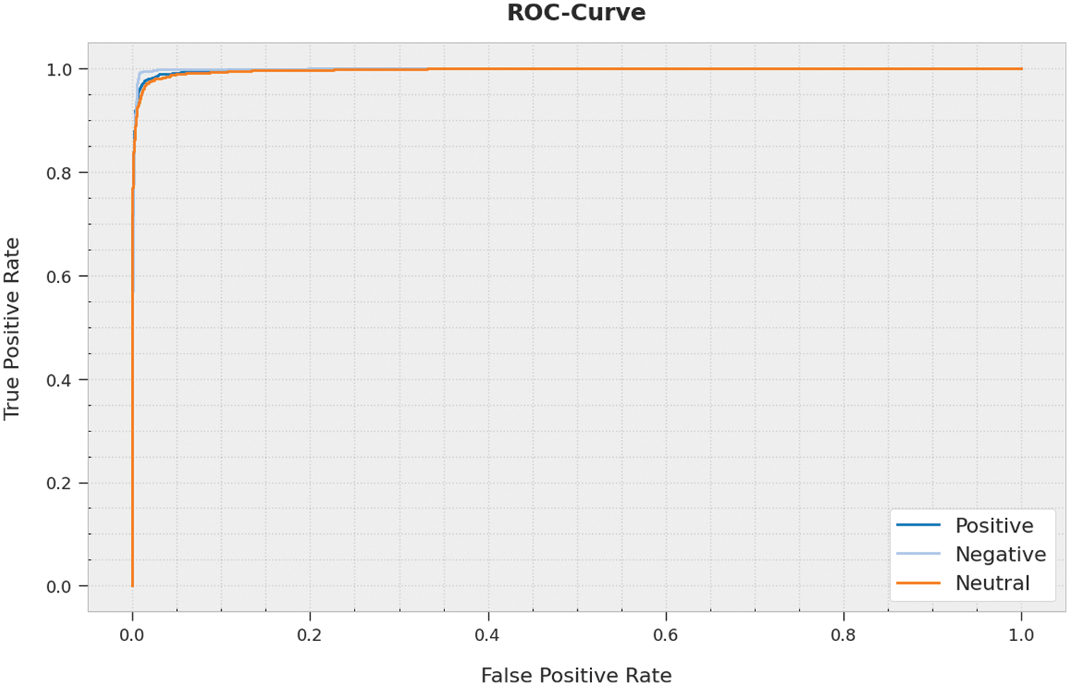
Figure 8: ROC curve analysis results of the IMDLSA-MR methodology

To emphasize the enhanced performance of the IMDLSA-MR method, a comparative accuy analysis was conducted against existing models such as the Naive Bayes (NB), k-nearest neighbor (KNN), Expectation–Maximization (ME), SVM, CNN, LSTM, Bidirectional LSTM (Bi-LSTM) and the CNN models and the results are shown in Table 3 and Fig. 9. The outcomes infer that the proposed IMDLSA-MR technique produced a maximum accuy of 98.92% whereas the NB, CNN, BiLSTM and the deep CNN approaches achieved the least accuy values such as 92.60%, 95.32%, 93.25% and 94.65% correspondingly. Meanwhile, it is shown that the SVM approach established a poor performance whereas the KNN and ME algorithms attained slightly improved results.

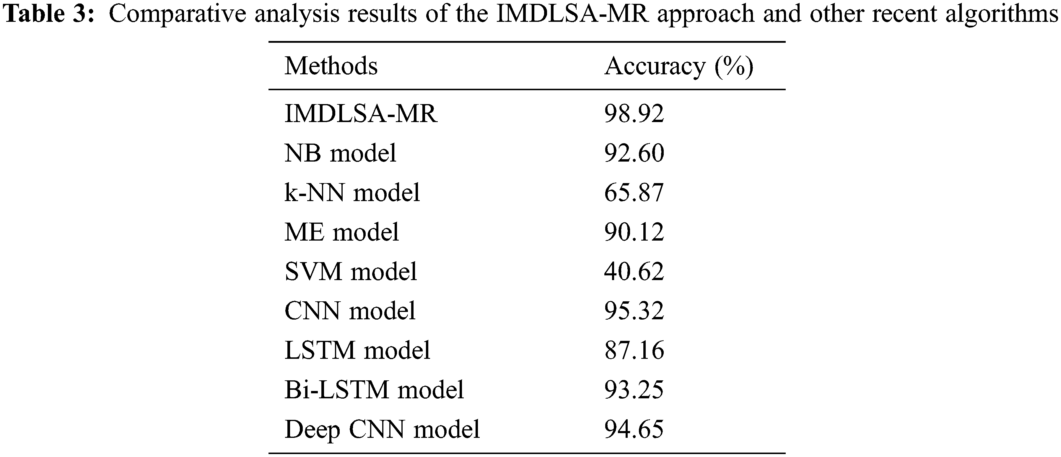
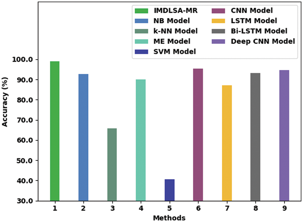
Figure 9: Comparative analysis results of the IMDLSA-MR approach and other recent algorithms

Finally, a detailed CT examination was conducted between the proposed IMDLSA-MR model and other existing models and the results are shown in Table 4 and Fig. 10. The results imply that the NB, KNN, SVM, LSTM, BiLSTM and the deep CNN models reported ineffectual outcomes with maximum CT values such as 155, 154, 163, 102, 179 and 120 s respectively. Next, the ME and CNN models produced slightly reduced CT values such as 85 and 84 s, respectively. However, the proposed IMDLSA-MR model achieved superior results with a minimal CT of 61 s. From the results and the detailed discussion, it can be inferred that the proposed IMDLSA-MR method achieved the maximum performance compared to other models.

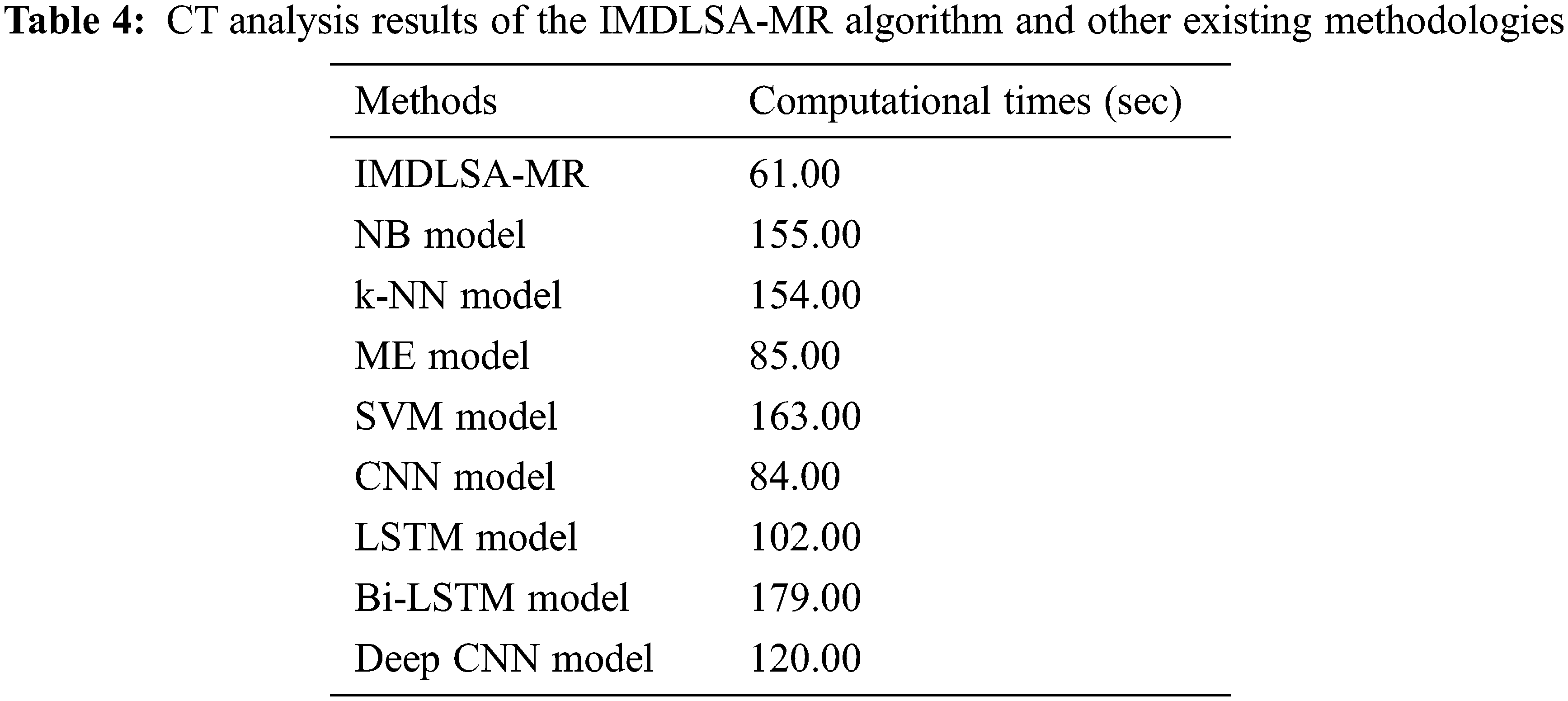
Figure 10: CT analysis results of the IMDLSA-MR algorithm and other existing methodologies

5  Conclusion

In this article, a new IMDLSA-MR method has been developed to analyse the sentiments on movie reviews using a standard movie reviews’ dataset. The presented IMDLSA-MR technique encompasses different phases such as data pre-processing, parameter optimization, feature extraction and the classification process. At the initial stage, the presented IMDLSA-MR technique applies different levels of pre-processing to convert the input data into a compatible format. Next, the TF-IDF model is exploited to generate the word vectors from the pre-processed data. Then, the DBN model is applied to analyse and classify the sentiments. At last, the IJSO technique is employed for optimal fine-tuning of the hyperparameters related to the DBN method. To establish the supreme performance of the proposed IMDLSA-MR model, numerous experimental analyses were conducted. The comparative study outcomes highlight the enhanced performance of the IMDLSA-MR model over recent DL models with a maximum accuracy of 98.92%. In the future, the performance of the proposed methodology can be enhanced by applying clustering and outlier removal approaches.

Funding Statement: Princess Nourah bint Abdulrahman University Researchers Supporting Project Number (PNURSP2023R161), Princess Nourah bint Abdulrahman University, Riyadh, Saudi Arabia. The authors would like to thank the ‎Deanship of Scientific Research at Umm Al-Qura University ‎for supporting this work by Grant Code: 22UQU4340237DSR51).

Conflicts of Interest: The authors declare that they have no conflicts of interest to report regarding the present study.

References

1. A. Jorio, S. E. Fkihi, B. Elbhiri and D. Aboutajdine, “An energy-efficient clustering routing algorithm based on geographic position and residual energy for wireless sensor network,” Journal of Computer Networks and Communications, vol. 2015, pp. 1–11, 2015. [Google Scholar]

2. K. Chakraborty, S. Bhattacharyya, R. Bag and A. Hassanien, “Sentiment analysis on a set of movie reviews using deep learning techniques,” Social Network Analytics: Computational Research Methods and Techniques, vol. 7, pp. 127–147, 2018. [Google Scholar]

3. D. Kansara and V. Sawant, “Comparison of traditional machine learning and deep learning approach for sentiment analysis,” in Advanced Computing Technologies and Applications, Algorithms for Intelligent Systems Book Series, Singapore: Springer, pp. 365–377, 2020. [Google Scholar]

4. K. Chakraborty, S. Bhattacharyya, R. Bag and A. E. Hassanien, “Comparative sentiment analysis on a set of movie reviews using deep learning approach,” in Int. Conf. on Advanced Machine Learning Technologies and Applications, Advances in Intelligent Systems and Computing Book Series, Cham: Springer, vol. 723, pp. 311–318, 2018. [Google Scholar]

5. S. Rani and P. Kumar, “Deep learning based sentiment analysis using convolution neural network,” Arabian Journal for Science and Engineering, vol. 44, no. 4, pp. 3305–3314, 2019. [Google Scholar]

6. N. C. Dang, M. N. M. García and F. De la Prieta, “Sentiment analysis based on deep learning: A comparative study,” Electronics, vol. 9, no. 3, pp. 483, 2020. [Google Scholar]

7. A. Yadav and D. K. Vishwakarma, “Sentiment analysis using deep learning architectures: A review,” Artificial Intelligence Review, vol. 53, no. 6, pp. 4335–4385, 2020. [Google Scholar]

8. L. Li, T. T. Goh and D. Jin, “How textual quality of online reviews affect classification performance: A case of deep learning sentiment analysis,” Neural Computing and Applications, vol. 32, no. 9, pp. 4387–4415, 2020. [Google Scholar]

9. D. Dessí, M. Dragoni, G. Fenu, M. Marras and D. R. Recupero, “Deep learning adaptation with word embeddings for sentiment analysis on online course reviews,” in Deep Learning-Based Approaches for Sentiment Analysis, Algorithms for Intelligent Systems Book Series, Singapore: Springer, pp. 57–83, 2020. [Google Scholar]

10. P. Patel, D. Patel and C. Naik, “Sentiment analysis on movie review using deep learning rnn method,” in Intelligent Data Engineering and Analytics, Advances in Intelligent Systems and Computing Book Series, vol. 1177, Singapore: Springer, pp. 155–163, 2021. [Google Scholar]

11. W. Li, B. Jin and Y. Quan, “Review of research on text sentiment analysis based on deep learning,” Open Access Library (OALib), vol. 7, no. 3, pp. 1–8, 2020. [Google Scholar]

12. H. Pouransari and S. Ghili, “Deep learning for sentiment analysis of movie reviews,” CS224N Project, pp. 1–8, 2014. [Google Scholar]

13. K. Dashtipour, M. Gogate, A. Adeel, H. Larijani and A. Hussain, “Sentiment analysis of Persian movie reviews using deep learning,” Entropy, vol. 23, no. 5, pp. 596, 2021 [Google Scholar] [PubMed]

14. N. M. Ali, M. M. A. E. Hamid and A. Youssif, “Sentiment analysis for movies reviews dataset using deep learning models,” International Journal of Data Mining & Knowledge Management Process (IJDKP), vol. 9, no. 3, pp. 19–27, 2019. [Google Scholar]

15. R. Bandana, “Sentiment analysis of movie reviews using heterogeneous features,” in 2018 2nd Int. Conf. on Electronics, Materials Engineering & Nano-Technology (IEMENTech), Kolkata, India, pp. 1–4, 2018. [Google Scholar]

16. U. D. Gandhi, P. M. Kumar, G. C. Babu and G. Karthick, “Sentiment analysis on twitter data by using convolutional neural network (CNN) and long short term memory (lstm),” Wireless Personal Communications, pp. 1–10, 2021. https://doi.org/10.1007/s11277-021-08580-3 [Google Scholar]

17. A. U. Rehman, A. K. Malik, B. Raza and W. Ali, “A hybrid CNN-lstm model for improving accuracy of movie reviews sentiment analysis,” Multimedia Tools and Applications, vol. 78, no. 18, pp. 26597–26613, 2019. [Google Scholar]

18. L. Zhu, L. Chen, D. Zhao, J. Zhou and W. Zhang, “Emotion recognition from Chinese speech for smart effective services using a combination of SVM and DBN,” Sensors, vol. 17, no. 7, pp. 1694, 2017 [Google Scholar] [PubMed]

19. J. S. Chou and D. N. Truong, “A novel metaheuristic optimizer inspired by behavior of jellyfish in ocean,” Applied Mathematics and Computation, vol. 389, pp. 125535, 2021. [Google Scholar]

20. H. A. Abdulwahab, A. Noraziah, A. A. Alsewari and S. Q. Salih, “An enhanced version of black hole algorithm via levy flight for optimization and data clustering problems,” IEEE Access, vol. 7, pp. 142085–142096, 2019. [Google Scholar]