Music Genre Classification Using DenseNet and Data Augmentation

1  Introduction

Today, advanced digital technology has dramatically changed how people create, distribute, enjoy, and consume music. On one hand, the number of musical works created by mankind is extremely large and constantly increasing. On the other hand, the musical genres are also very rich. Therefore, manually sorting, classifying, and searching for such musical works is an extremely difficult, if not impossible, task. Computers, machine learning, and deep learning tools have enabled such tasks to be performed automatically. In addition, various music data sets have been developed, which are very helpful for research in this area.

Traditional classifiers can be used for music genre classification problems; however, with the strong advancement of technology, deep learning classifiers have provided outstanding results. On the data side, depending on the nature of the data, there are appropriate data augmentation methods that improve recognition or classification accuracy [1,2]. According to [1,2], appropriate data augmentation improves classification accuracy. In addition, data augmentation is required to increase the amount of memory and the training time.

This paper presents research that classifies music genres using deep learning tools and effective data augmentation methods for the Small FMA data set. The rest of the paper is organized as follows: Section 2 discusses related work. Section 3 describes the data augmentation methods for Small FMA. Section 4 describes the models used in experiments. Section 5 presents the results and a discussion. Finally, Section 6 concludes the paper.

2  Related Work

The FMA was introduced by Defferrard et al. in [3]. FMA is a large-scale data set for evaluating several tasks in music information retrieval. It consists of 343 days of audio from 106,574 tracks by 16,341 artists on 14,854 albums arranged in a hierarchical taxonomy of 161 genres. It provides full-length, high-quality audio, pre-computed features, tracks, user-level metadata, tags, and free-form text such as biographies. There are four subsets defined by the authors: full, the complete data set; large, the full data set with audio limited to 30-s clips extracted from the middle of the tracks (or entire track if shorter than 30 s); medium, a selection of 25,000 30-s clips with a single root genre; and small, a balanced subset containing 8,000 30-s clips, with 1,000 clips per one of eight root genres. The eight root genres are electronic, experimental, folk, hip-hop, instrumental, international, pop, and rock.

Owing to hardware constraints, Small FMA was used in this study. For comparison with other studies, this section also presents research that has used the same Small FMA in recent years. More details on related research are presented in Table 1 (at the end of this study). The models used for Music Genre Classification (MGC) and Small FMA are described below. The authors of [4] used a Bayesian network, whereas Wang [5], Ke et al. [6] used SVM [7] for MGC. Most studies have used deep neural networks (DNNs) for MGC. Convolutional Neural Networks (CNNs) were originally used for image processing [8,9] but were also used for MGC [10–12]. The research in [13–15] used Convolutional Recurrent Neural Networks (CRNNs). In [16], Bottom-up Broadcast Neural Networks (BBNNs) were used. The authors in [17] exploited LSTM and DenseNet was used in [18]. In [19], a Siamese neural network [20] was used, which is made up of twin networks that share weights and configurations before providing unique inputs to the network and optimizing similarity scores. Most authors used the Mel spectrogram for the feature parameters, as in [6,10,12–17,21]. Others have used spectrograms, as in [11,18,22]. Pimenta-Zanon et al. [4] used EXAMINNER for the feature extraction. The authors of [23] used 500 features from the FMA data set for their research. An approach in MGC that is not yet popular is the classification of detailed sub-genres. ResNet18b, MobileNetV3, VGG16, DenseNet121, ShuffleNetV2, and vision transformers (ViT) with a Mel spectrogram were used in [24] for the classification of sub-genres: FH (future house), BH (bass house), PH (progressive house), and MH (melodic house). In [24], the highest accuracy was 75.29% with ResNet18b.

With the content presented above, it can be seen that in addition to traditional classifiers, innovations in deep learning have been used in MGC, from early models of deep learning such as CNN, CRNN, and LSTM to later variants with more complex architectures such as GRU, Siamese neural networks, ResNet, and DenseNet. In addition to using the Mel Spectrogram as a feature parameter for MGC, other features in the time and frequency domains [25] were also exploited. Features in the frequency domain include spectral bandwidth, spectral centroid, spectral roll-off, and Mel frequency cepstral coefficients (MFCCs). In the time domain, the commonly used feature parameters are the zero-crossing rate, short-time energy, tempo, and root-mean-square energy. Chroma-based parameters also represent the tonal content of a musical audio signal in condensed form. In machine learning and deep learning, models are important for solving classification and recognition problems. However, a good model with poor data quality and a lack of data will make it difficult to achieve good results. Few studies have used appropriate data-enhancement methods when using Small FMA for MGC. Data augmentation for Small FMA is detailed later in this paper.

3  Proposed Data Augmentation Methods

Among the studies listed in Table 1, only [14,18] used data augmentation in their study. Pitch shifting was used for data augmentation in [14,18]. The data augmentation methods used in this study include adding noise, creating echoes, and changing the pitch. Among these methods, changing the pitch proved to be less effective than the other two methods, as seen in the experimental section. The following is a description of the data augmentation methods implemented in this study.

•   For noise addition, Librosa [26] was used.

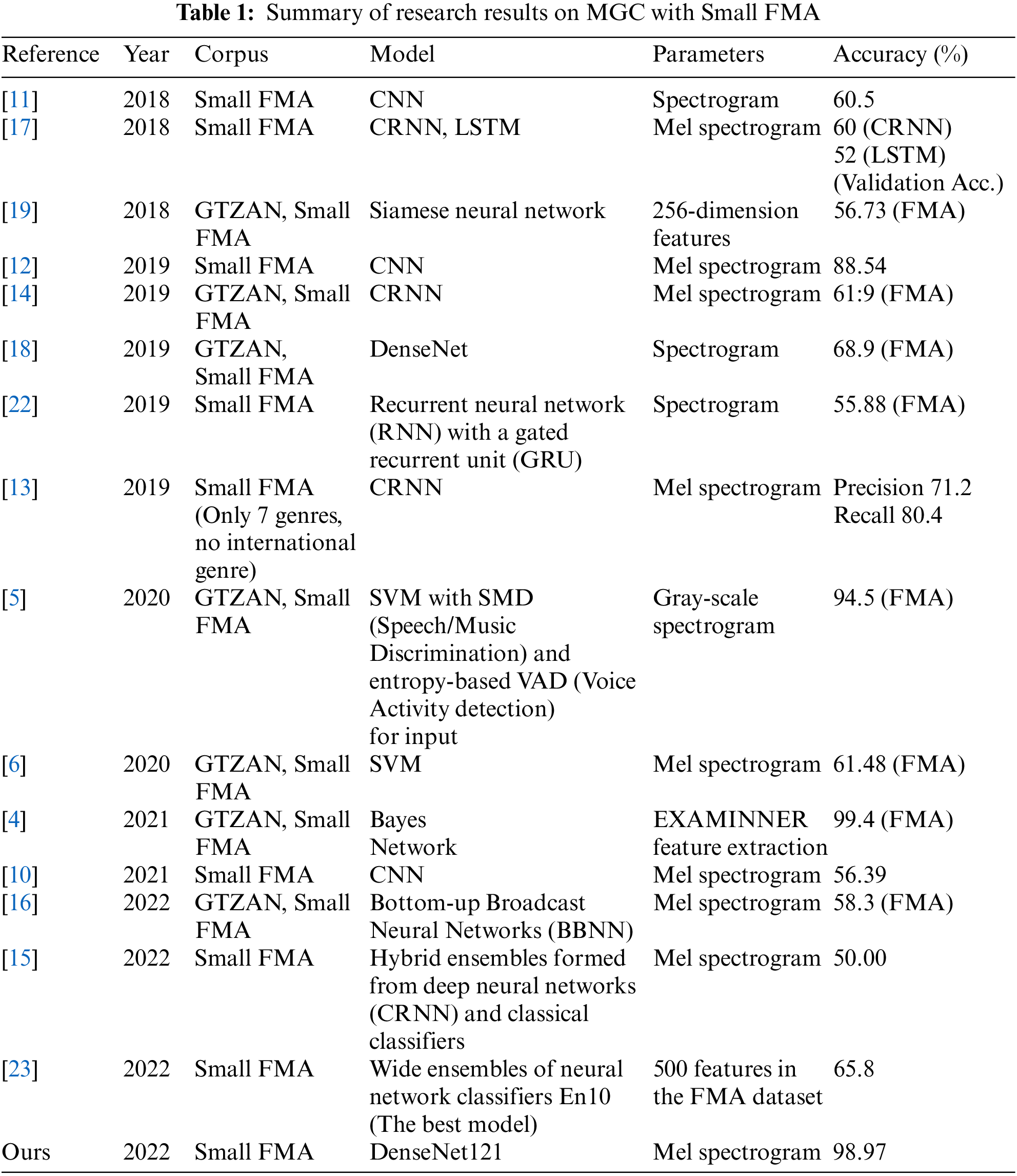
The amplitude of the white noise is taken as 0.03 of the signal’s peak amplitude, and then this noise is added to the signal. The signal-to-noise ratio (SNR) was calculated using the following formula: SNR(dB)=10log10PSPN where PS is the signal power and PN is the added noise power with the assumption that the background noise that exists in the original sound files can be ignored. From there, the average SNR of 8000 sound files was approximately 19.38 dB. According to the International Computer Science Institute (ICSI) [27], an SNR of 30 dB was considered a clean signal. Thus, the addition of noise degrades the quality of the signal, but not significantly in this case. Fig. 1 shows an example of calculating a file’s SNR and its average.

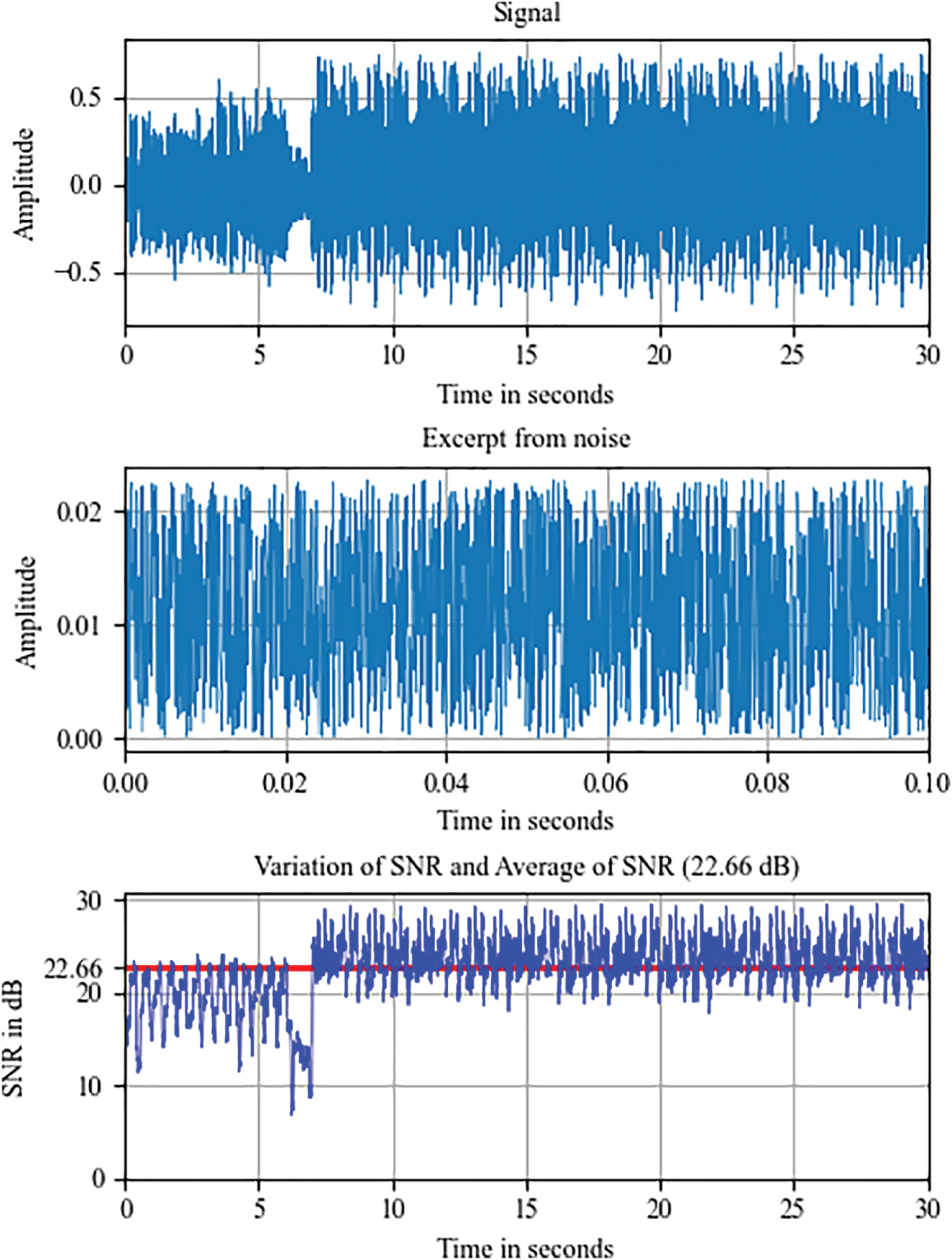
Figure 1: An example of calculating the SNR and its average for a file

•   Creating echo

The echo effect causes a sound to repeat with a delay and diminishing volume, simulating the real effect of an echo. In this study, the sound signal was delayed by 250 ms and repeated thrice. For each iteration, the delay amplitude was multiplied by a factor of 0.25. Fig. 2 illustrates the echo generated at the end of the sound file.

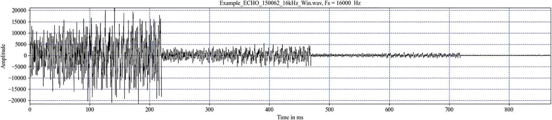
Figure 2: Echo generated at the end of the sound file

•   Changing pitch

Pitch change is achieved by pitch-shifting by a semitone or a tone. The librosa.effects.pitch_shift from Librosa was used for this purpose. To illustrate pitch shifting, Fig. 3 shows the upward shift of the A5 note. The A5 note has a frequency of 880 Hz. After shifting to a semitone, there is an A5 with a frequency of 933.88 Hz. The A5 note became a B5 note after shifting up one note, with a frequency of 987.77 Hz.

Figure 3: Illustration of shifting up a semitone and a tone

4  Proposed Models for Our Experiments

In this study, the MGC problem becomes an image recognition problem by transforming the sound files into corresponding Mel spectrograms. The Mel spectrograms of the sound files are the input images for the proposed recognition models. A spectrogram is a visual representation of signals in three dimensions: time, frequency, and amplitude. A Mel spectrogram is a spectrogram that is converted to a Mel scale. The human auditory system perceives frequencies on a logarithmic scale rather than a linear scale [28]. Fig. 4 shows an example of a Mel spectrogram for a wave file.

Figure 4: Mel spectrogram of a wave file

The models used to perform the experiments include DenseNet, CNN, and GRU (Gated Recurrent Units). Three variants of DenseNet were used: DenseNet121, DenseNet169, and DenseNet201 [29]. The DenseNet model is briefly described as follows:

DenseNet is one of the seven best models for image classification using Keras [30]. In a traditional CNN, the input image is passed through the network to extract feature mappings in turn. Finally, labels on the output are predicted in a way where the forward pass is straightforward. Except for the first convolutional layer, whose input is the image to be recognized, each layer uses the output of the previous layer to create a feature map in the output. This feature map is then passed to the next convolutional layer. If the CNN network has L layers, there will be L connections between one layer and the next. Fig. 5 shows an illustration of the DenseNet architecture.

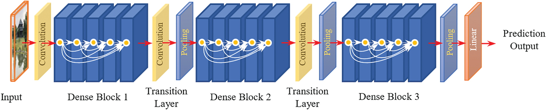
Figure 5: Illustration of DenseNet architecture

DenseNet [31] introduced Densely Connected Neural Networks to obtain deeper insights, efficient and accurate training, and outputs. For DenseNet, in addition to the connection between layers, such as the connection in a CNN, there is another special type of connection. In DenseNet architecture, each layer is connected to every other layer. If DenseNet has L layers, then there will be L(L+1)/2 direct connections. The input of a layer inside DenseNet is the concatenation of feature maps from the previous layers.

The architecture of DenseNet contains dense blocks, where the dimensions of the feature maps remain constant within a block but the number of filters changes between them. Transition Layers were used to connect the dense blocks.

As shown in Table 1 from [31], DenseNet121 has (6, 12, 24, 16) layers in four dense blocks. The number 121 is calculated as 5 + (6 + 12 + 24 + 16) × 2 = 121, where 5 represents (convolution, pooling) + 3 transition layers + classification layers. Multiplying by two is necessary because each dense block has two layers (1 × 1 convolution and 3 × 3 convolution). The same can be inferred for DenseNet169 and DenseNet201.

The CNN model in this study inherits the CNN model used and presented in [1]. The same applies to the GRU model used and presented in [1]. In this study, the input image sizes for the CNN and GRU models are (230 × 230).

5  Results and Discussions

Section 5 presents the results of the experiments as follows. First, DenseNet169 is used for MGC with data augmented four times and for two sampling frequencies of sound files, 44100 and 16000 Hz. The results of this experiment show that a sampling frequency of 16000 Hz gives better classification accuracy than a sampling frequency of 44100 Hz. Therefore, all subsequent experiments on DenseNet121, DenseNet169, DenseNet201, CNN, and GRU were performed using data with a sampling frequency of 16000 Hz. Next, to better observe the effectiveness of data augmentation, the experiments were performed with data augmented three times, twice, and without data augmentation. Finally, experimental results with data augmented by pitch shifting are presented.

5.1 Data with Sampling Frequency fs = 44100 Hz and fs = 16000 Hz

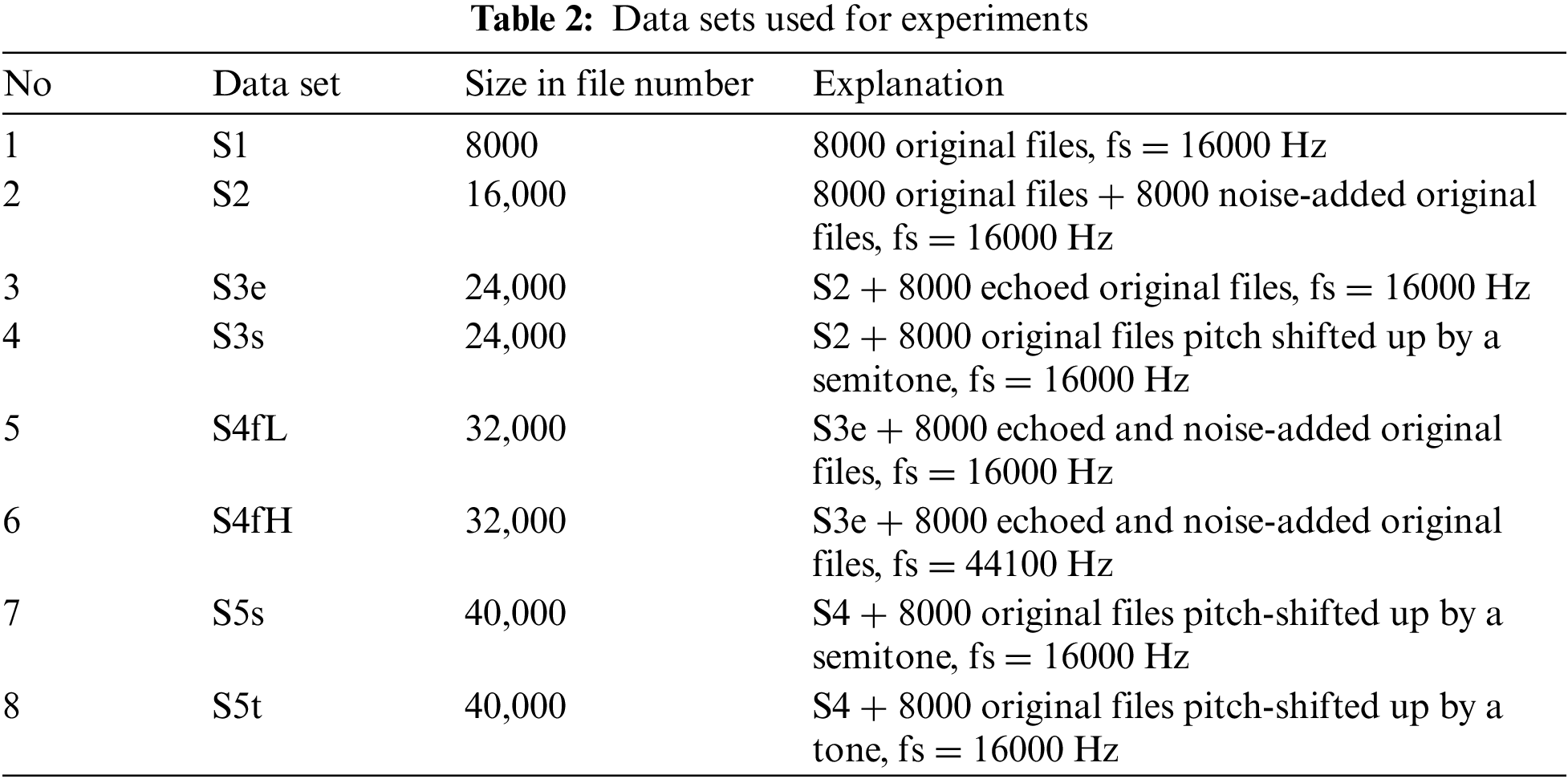
The data sets used in this study are listed in Table 2. First, the DenseNet169 model is used for Small FMA with two data sets, S4fH and S4fL. These two data sets both contain 4-fold enhanced data and differ only in sampling frequency, as shown in Table 2. A total of 32,000 files from each data set were divided into 10 parts for cross-validation. One of the 10 parts was segregated and used for testing. The remaining nine were used for training and validation with a training:validation ratio of 8:1. Thus, there were nine folds for training and validation.

If the sampling frequency was 44100 Hz and the duration of each file was 30 s, the number of samples in each file was 30×4410=1,323,000 samples. If the frame width used to calculate the FFT for the Mel spectrum is 4028 samples and the frameshift is 2014 samples, the corresponding number of frames for a sound file is 646. Thus, each audio file was converted into an image file of size 646 (number of Mel coefficients) × 646 (number of frames). In this study, the input shape for use with DenseNet networks had a target of (224, 224, 3). (224, 224): image size; (3): three images (R, G, and B). The quantities such as accuracy, precision, recall, and f1-score in this study are calculated according to [32]. Table 3 is the average values (%) for nine folds of precision, recall, f1-score, accuracy, and Area Under the Receiver Operating Characteristics (AUC) [33,34] for Densenet169 with the data set S4fH.

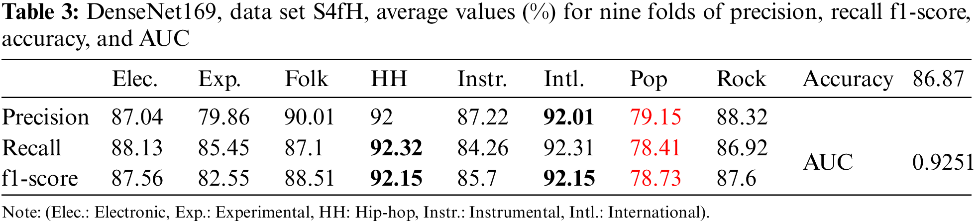
Table 3 shows that precision achieved the highest value (in bold) of 92.01% for the international genre but recall and f1-score had the highest value for the same genre of hip-hop. Precision, recall, and f1-score had the same lowest value (in red) for the pop genre.

If the sampling frequency is reduced to 16000 Hz, the number of samples in each file is 30 × 16000 = 480,000. If the frame width and the frameshift remain the same, then the corresponding number of frames for a sound file will be approximately 234. To prevent the number of samples from possibly exceeding the size of the sound file, the number of frames was 230. Thus, each sound file was converted to an image file of size 230 (number of Mel coefficients) by 230 (number of frames). The input shape for use with DenseNet networks remains the same (224, 224, 3). The average values (%) of accuracy, AUC, precision, recall, and f1-score for nine folds are presented in Table 4.

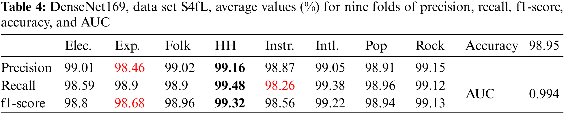
From Table 4, the precision, recall, and f1-score all have the same highest value (in bold) for the hip-hop genre. The lowest values (in red) are for precision and f1-score of the experimental genre and recall of the instrumental genre. It can be observed that reducing the sampling frequency to 16000 Hz leads to a reduction in image size and a significant increase in recognition accuracy. Therefore, the experiments in this study were performed with a sampling frequency of 16000 Hz.

Table 5 displays the results of DenseNet121 with image size (230 × 230) and data set S4fL.

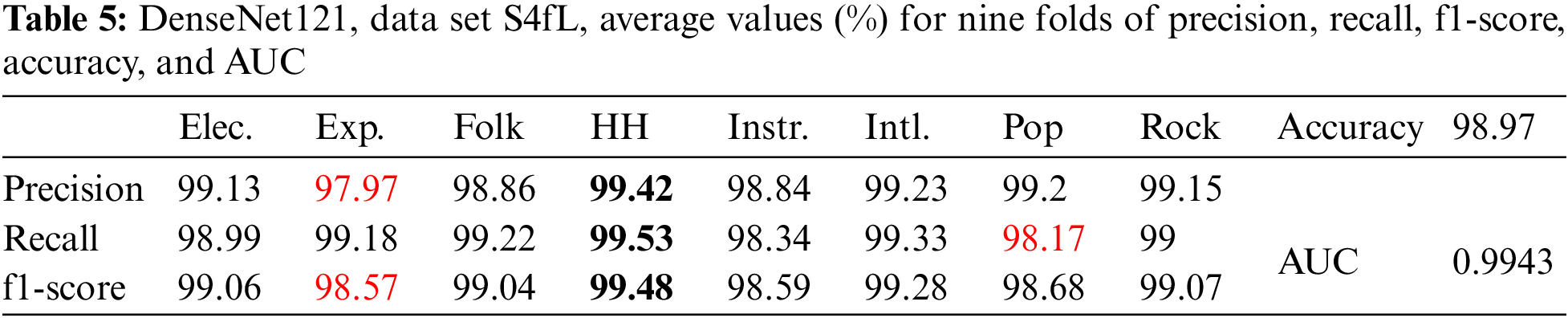
The precision, recall, and f1-score from Table 5 had the highest value for the same hip-hop genre. The lowest values were for precision and f1-score in the experimental genre and recall in the pop genre.

Table 6 shows the results for DenseNet201 with image size (230 × 230) and data set S4fL.

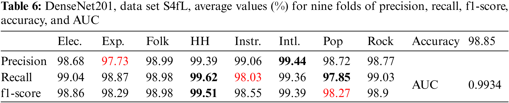
For DenseNet201 with data set S4fL, as shown in Table 6, it can be seen that recall and f1-score have the highest value for the hip-hop genre, while precision has the highest value for the international genre. The lowest values are for precision with the experimental genre, recall with the instrumental genre, and f1-score with the pop genre.

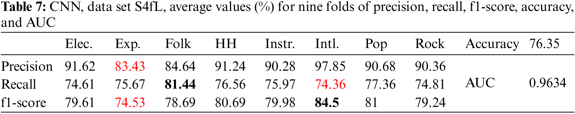
Table 7 displays the results for the CNN model with image size (230 × 230) and data set S4fL. The highest values were for precision and f1-score in the international genre and recall in the folk genre. The lowest values were for precision and f1-score in the experimental genre and recall in the international genre.

The following Table 8 shows the results for the GRU model with image size (230 × 230) and data set S4fL.

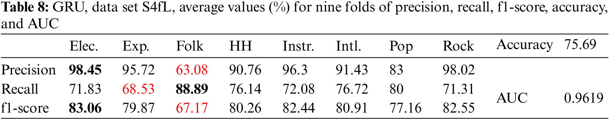
For the GRU model, as shown in Table 8, precision and f1-score had the highest value for the electronic genre, while recall had the highest value for the folk genre. Precision and f1-score had the lowest value for the same folk genre, while recall had the lowest value for the experimental genre.

A summary of the accuracies of DenseNet169, DenseNet121, DenseNet201, CNN, and GRU is depicted in Fig. 6.

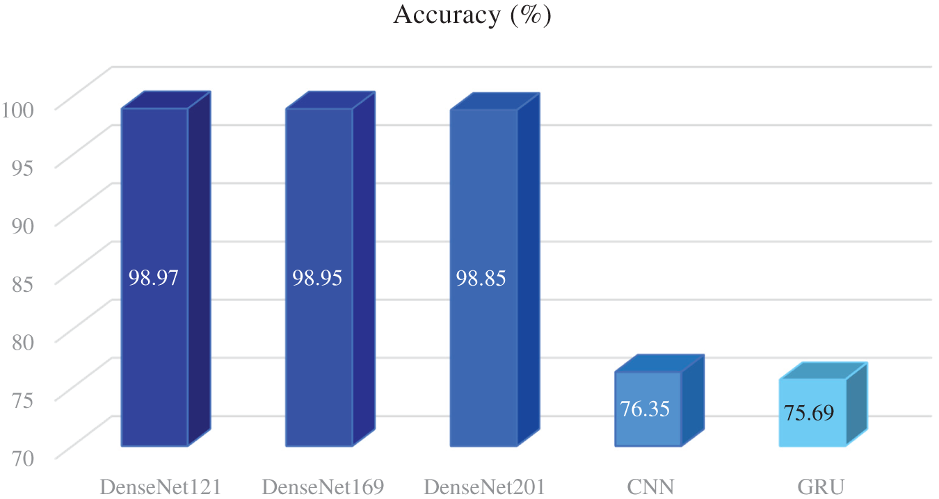
Figure 6: Summary of the accuracy of models with the data set S4fL

Thus, DenseNet121 gives the highest accuracy of 98.97% with the data set S4fL, and this accuracy is superior to most of the studies given in Table 1, exception for [4]. Fig. 7 is an illustrative quote for the classification results of DenseNet121 with the data set S4fL, including the variation of training loss and validation loss according to epoch, the confusion matrix, and ROC curves for Fold 6. Note that the closer the AUC is to 1, the better [35].

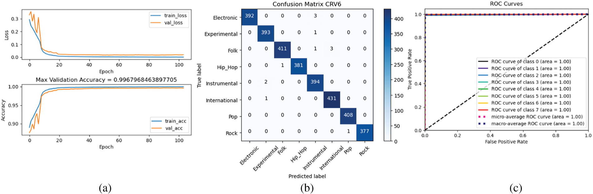
Figure 7: (a) Variations of training loss and validation loss according to epoch (b) confusion matrix (c) ROC curves

From Fig. 7a it can be seen that the variations in the training losses according to the epoch match variations in the validation losses. The same is true for the variations in the training accuracy and validation accuracy by epoch. This demonstrates that overfitting did not occur [35].

5.2 Effect of Data Augmentation

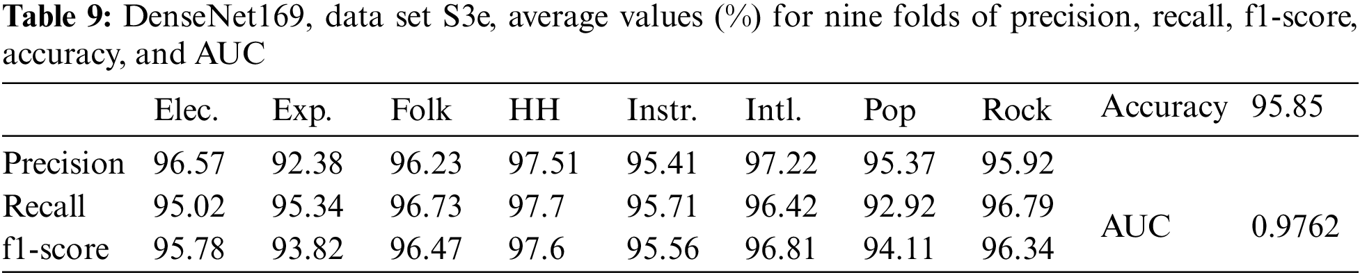
To better understand the effect of data augmentation, the experiments were performed with three data sets, S3e, S2, and S1, for DenseNet169. Table 9 displays the results for DenseNet169 with image size (230 × 230) and data set S3e. These results show that the average values of accuracy, AUC, precision, recall, and f1-score were all lower than those of data set S4fL.

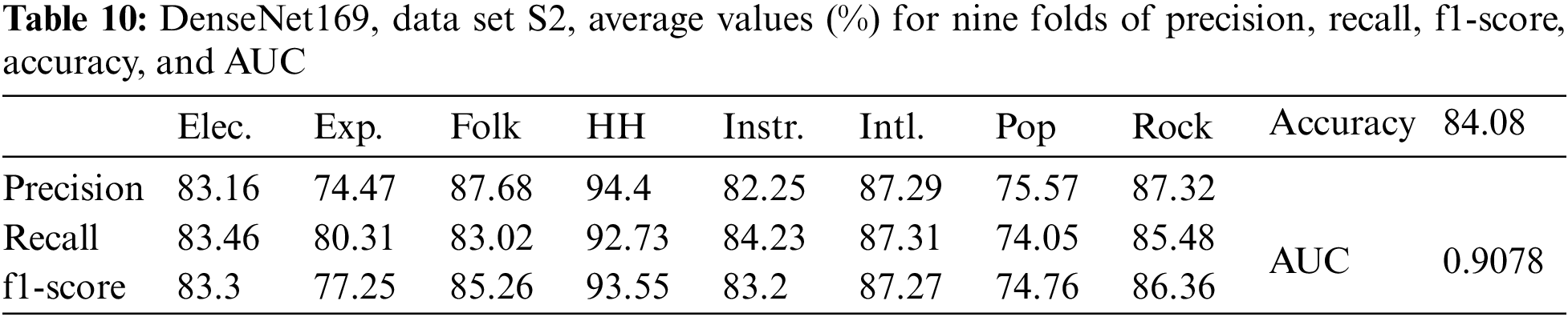
The results for DenseNet169 with data set S2 are presented in Table 10. The average values of accuracy, AUC, precision, recall, and f1-score, in this case, were all lower than those of DenseNet169 with data set S3e.

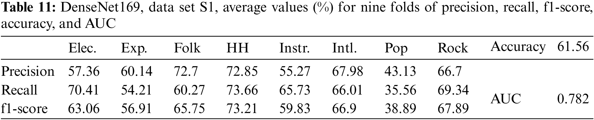
In the absence of data augmentation, the results for DenseNet169 with data set S1 and image size (230×230) are given in Table 11. In this case, the average values of accuracy, AUC, precision, recall, and f1-score were the lowest compared to the above data augmentation cases.

The MGC accuracy of the DenseNet169 model according to augmented data size is shown in Fig. 8.

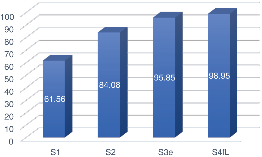
Figure 8: The MGC accuracy of the DenseNet169 model depends on the data size

As shown in Fig. 8, the MCG accuracy increased as the data size increased from two to four times.

5.3 Data Augmentation with Pitch Shifting

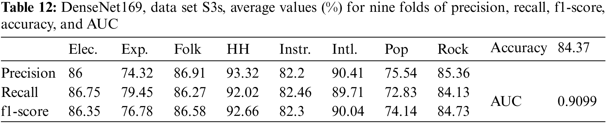
As shown above, for data set S3e, the data were increased by three times by adding noise and creating an echo. To compare the method of data augmentation by echoing with pitch shifting, an experiment was carried out with the data size increased three times by adding noise and pitch shifting. First, the original data were shifted up using a semitone. Therefore, the data set was S3s. The results from Table 12 show that the classification accuracy for the data set S3s is increased in comparison with S2, but not so much. On the other hand, the classification accuracy for data set S3s is lower than that for S3e. Thus, it can be said that in this case, the data augmented by pitch shifting is less efficient than that augmented by echo generation.

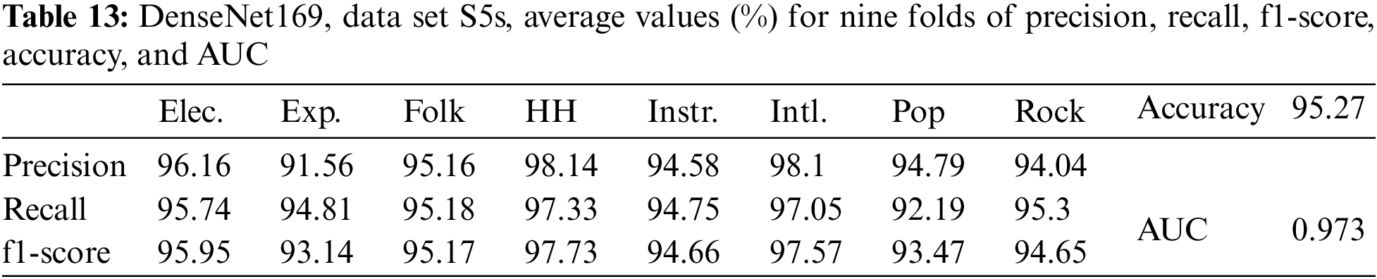
Finally, an experiment was conducted by increasing the data size by five times. By pitch shifting, the data size was increased by five times, with a total of 40000 files. The pitch was raised by a semitone for data set S5s and a tone for data set S5t.

Table 13 shows the results for DenseNet169 with image size (230 × 230) and data set S5s. These results show that increasing the data by a fifth time by shifting up a semitone did not improve the accuracy when compared to only increasing the data four times.

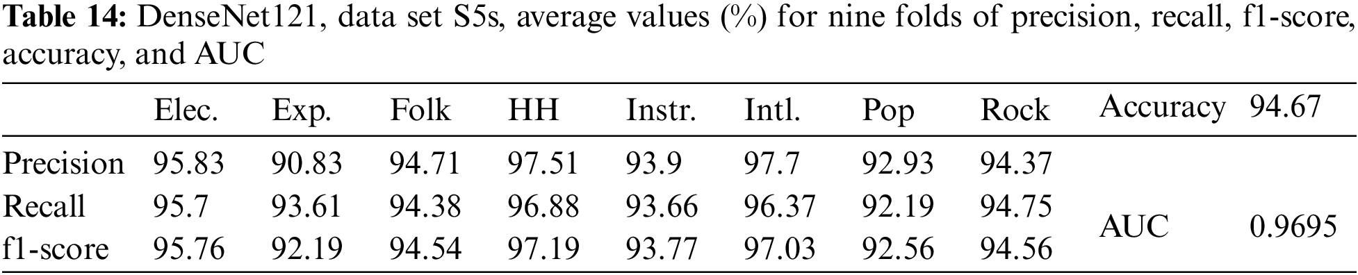
The above comment is also true for Denset121 with the data set S5s, where the results are given in Table 14.

The final experiment we would like to present here is for the data set S5t. Table 15 shows the results in this case for DenseNet121.

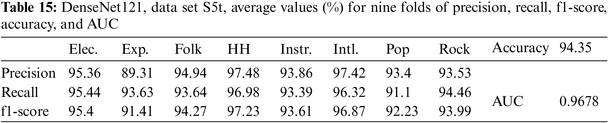
With two data sets, S5s and S5t, some observations can be made as follows: For DenseNet169, the accuracy of 95.27% with data set S5s was higher than the accuracy of 94.67% for DenseNet121. For DenseNet121, the accuracy of 94.35% with data set S5t is lower than the accuracy of 94.67% with data set S5s. Thus, data augmentation by pitch-shifted up by one tone did not lead to a better classification accuracy than pitch-shifted up by a semitone. This is also consistent with the comments in [18], which stated that “with a small change of pitch of a song, its classification still works,” and [18] only used shifting the pitch of songs by half a tone.

There have been studies on the computational cost of deep learning models [36], the model complexity of deep learning [37,38], and the methods to reduce the computational complexity of deep learning [39,40]. A full analysis of the time complexity of the entire algorithm of the models such as DenseNet121, DenseNet169, and DenseNet201 is beyond the scope of this work. On the other hand, in this study, there is no algorithmic change in the aforementioned models. In this study, the size of the data used for training was increased. This increases the training time. Therefore, this paper only compares the training time for two cases: augmented and unaugmented data.

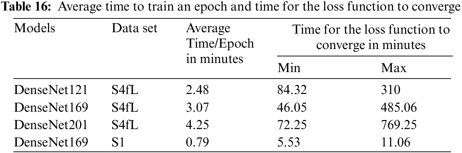
The hardware configuration for this study was as follows: Intel Core i7-8700K @3.2 GHz, 12 threads of processing power, 32 GB of RAM, 2 TB of storage, and NVIDIA GeForce RTX 2080 Ti with 11 GB of RAM. The following software versions were used: Ubuntu 19.10, Python 3.8, Keras 2.4.3, Tensorflow 2.3.0, Tensorflow-GPU 2.3.0, and Librosa 0.7.2. Table 16 gives the average time to train an epoch and the time for the loss function to converge with two data sets, S4fL and S1. For the model DenseNet169 and data set S1, the average training time for one epoch is 0.79 min. If the data are increased by four times (the data set S4fL), this time is 3.07 min. Therefore, increasing the data by four times resulted in an increased training time of approximately 3.07/0.79 ≈ 3.89 times for one epoch. The time required for each model for the loss function to converge depends on the size of the data and fold. For the model DenseNet169, the maximum values of this time are 485.06 and 11.06 min with the data sets S4fL and S1, respectively. Also, with the model DenseNet169, the maximum time for the loss function to converge is increased by about 485.06/11.06 ≈ 43.86 times if the size of the data is increased by 4 times. On average, in this case, the DenseNet121 model’s computational speed was the fastest, and that of the DenseNet201 model was the slowest.

To conclude Section 5, the following is a discussion of the addition of white noise to enhance the data and the reduction of the sampling frequency of the data to 16000 Hz that was performed in this study. One assumption made clear in this study is that the background noise that exists in the original sound files can be ignored. Therefore, what will happen if this background noise has a large value? This study used a white noise addition method to enhance the data. If the background noise in the original sound files is too large, adding noise increases the risk of reducing the quality of the audio files. This significantly distorts the image quality of the data-enhanced audio file compared to the image quality of the original file. This adversely affects the training and testing processes, making it difficult to achieve a high classification accuracy. The experimental results showed that this was not the case. By adding white noise with an appropriate amplitude, the classification accuracy was increased compared with the case where the data were not enhanced by noise addition. The drawback of data augmentation is that it increases the training time.

This study reduced the sampling frequency of the data from 44100 to 16000 Hz. Under what assumptions would one be able to do so while maintaining high classification accuracy? The sampling frequency of the original audio file is 44100 Hz. According to the Nyquist-Shannon sampling theorem [41], the peak frequency of the audio signal, in this case, is fs/2 = 22050 Hz. This peak frequency is close to the maximum frequency that the human cognitive system can perceive. The problem posed in this study was MGC. To recognize musical genres, the human auditory system does not need to absorb all the details of the information contained in the sound but usually only requires general information. Therefore, in this case, the MGC still achieved good results. However, if the problem is to identify the singer's voice, more detailed information will be required in the signal spectrum. In this case, if the sampling frequency is reduced too low, the detailed information contained in the signal spectrum will be lost. As a result, singer voice recognition will be inconvenient, and it may be difficult to achieve high accuracy.

The source code for this research and user guide are available at the following link: https://drive.google.com/drive/folders/1UR_X8fq8U0aiNWVobTzNCZeWe4Iae3ti?usp=sharing.

6  Conclusions

The research results presented in this paper demonstrate that appropriately defining the deep learning model in conjunction with an efficient data augmentation method enables MGC accuracy to outperform the majority of the available studies on the same Small FMA data set. The music genre classification problem in this research becomes an image recognition problem in which each musical work is characterized by the corresponding Mel spectrogram. Reducing the sampling frequency of the original sound files from 44100 to 16000 Hz allows for a reduction in the size of the image to be recognized and increases the recognition accuracy. DenseNet121 provided the highest recognition accuracy with 4-fold enhanced data among the deep learning models. The experiments also show that data augmentation by echoing is more effective than pitch shifting in increasing classification accuracy. However, pitch-shifting up by one tone does not improve classification accuracy compared to pitch-shifting up by a semitone. Our future work will involve exploiting other sources of music data and finding ways to improve the accuracy of music genre classification. In addition to data enhancement methods, studies will be conducted to reduce the computational complexity of deep learning models.

Acknowledgement: This research is funded by the University of Transport and Communications (UTC) under grant number T2022-CN-006. We would like to express our gratitude to UTC and the Faculty of Information Technology (FIT).

Funding Statement: The authors received the research fun T2022-CN-006 for this study.

Conflicts of Interest: The authors declare that they have no conflicts of interest to report regarding the present this study.

References

1. V. L. Trinh, T. L. T. Dao, X. T. Le and C. Eric, “Emotional speech recognition using deep neural networks,” Sensors, vol. 22, no. 4, pp. 1–20, 2022. [Google Scholar]

2. V. L. Trinh, H. Q. Nguyen and T. L. T. Dao, “Emotion recognition with capsule neural network,” Computer Systems Science and Engineering, vol. 41, no. 3, pp. 1083–1098, 2022. [Google Scholar]

3. M. Defferrard, K. Benzi, P. Vandergheynst and X. Bresson, “FMA: A dataset for music analysis,” arXiv preprint arXiv:1612.01840, 2016. [Google Scholar]

4. M. H. Pimenta-Zanon, G. M. Bressan and F. M. Lopes, “Complex network-based approach for feature extraction and classification of musical genres,” arXiv preprint arXiv:2110.04654, 2021. [Google Scholar]

5. K. C. Wang, “Robust audio content classification using hybrid-based SMD and entropy-based VAD,” Entropy, vol. 22, no. 2, pp. 1–23, 2020. [Google Scholar]

6. C. Ke and L. Beici, “Do user preference data benefit music genre classification tasks?,” in Proc. the 21st Int. Society for Music Information Retrieval Conf., Montréal, Canada, 2020. [Google Scholar]

7. B. E. Boser, I. M. Guyon and V. N. Vapnik, “A training algorithm for optimal margin classifiers,” in Proc. of the Fifth Annual Workshop on Computational Learning Theory, Pittsburgh, Pennsylvania, USA, pp. 144–152, 1992. [Google Scholar]

8. A. Amirkhani, A. H. Barshooi and A. Ebrahimi, “Enhancing the robustness of visual object tracking via style transfer,” CMC-Computers, Materials & Continua, vol. 70, no. 1, pp. 981–997, 2022. [Google Scholar]

9. A. Amirkhani and A. H. Barshooi, “DeepCar 5.0: Vehicle make and model recognition under challenging conditions,” IEEE Transactions on Intelligent Transportation Systems, vol. 24, no. 1, pp. 541–553, 2022. [Google Scholar]

10. D. Kostrzewa, P. Kaminski and R. Brzeski, “Music genre classification: Looking for the perfect network,” in Int. Conf. on Computational Science, Cham, Springer, pp. 55–67, June 2021. [Google Scholar]

11. M. Matocha and S. K. Zieliński, “Music genre recognition using convolutional neural networks,” Advances in Computer Science Research, vol. 14, pp. 125–142, 2018. [Google Scholar]

12. S. Chillara, A. S. Kavitha, S. A. Neginhal, S. Haldia and K. S. Vidyullatha, “Music genre classification using machine learning algorithms: A comparison,” International Research Journal of Engineering and Technology (IRJET), vol. 6, no. 5, pp. 851–858, 2019. [Google Scholar]

13. A. A. Gunawan and D. Suhartono, “Music recommender system based on genre using convolutional recurrent neural networks,” Procedia Computer Science, vol. 157, no. 2, pp. 99–109, 2019. [Google Scholar]

14. Y. Qin and A. Lerch, “Tuning frequency dependency in music classification,” in ICASSP 2019-IEEE Int. Conf. on Acoustics, Speech, and Signal Processing (ICASSP), Brighton, UK, pp. 401–405, May 2019. [Google Scholar]

15. D. Kostrzewa, M. Ciszynski and R. Brzeski, “Evolvable hybrid ensembles for musical genre classification,” in Pro. Genetic and Evolutionary Computation Conf. Companion, Boston, MA, US, pp. 252–255, 2022. [Google Scholar]

16. A. Heakl, A. Abdelrahman and P. Victor, “A study on broadcast networks for music genre classification,” arXiv preprint arXiv:2208.12086, 2022. [Google Scholar]

17. V. Choudhary and A. Vyas, “CS543: Music genre recognition through audio samples,” small, vol. 8, no. 8, pp. 1–6, 2018. [Google Scholar]

18. W. Bian, J. Wang, B. Zhuang, J. Yang, S. Wang et al., “Audio-based music classification with DenseNet and data augmentation,” in Pacific Rim Int. Conf. on Artificial Intelligence, Cham, Springer, pp. 56–65, 2019. [Google Scholar]

19. J. Park, L. Jongpil, P. Jangyeonk, H. Jung-Woo and N. Juhan, “Representation learning of music using artist labels,” in Proc. the 19th ISMIR Conf., Paris, France, pp. 717–724, September 23–27, 2018. [Google Scholar]

20. D. Chicco, “Siamese neural networks: An overview,” Artificial Neural Networks, vol. 2190, pp. 73–94, 2021. [Google Scholar]

21. D. Kostrzewa, M. Ciszynski and R. Brzeski, “Evolvable hybrid ensembles for musical genre classification,” in Proc. Genetic and Evolutionary Computation Conf. Companion, Boston, MA, US, pp. 252–255, 2022. [Google Scholar]

22. Y. Yi, K. Y. Chen and H. Y. Gu, “Mixture of CNN experts from multiple acoustic feature domain for music genre classification,” in Asia-Pacific Signal and Information Processing Association Annual Summit and Conf. (APSIPA ASC), Lanzhou, China, IEEE, pp. 1250–1255, 2019. [Google Scholar]

23. D. Kostrzewa, W. Mazur and R. Brzeski, “Wide ensembles of neural networks in music genre classification,” in Int. Conf. on Computational Science, Cham, Springer, pp. 64–71, 2022. [Google Scholar]

24. X. Li, “HouseX: A fine-grained house music dataset and its potential in the music industry,” arXiv preprint arXiv:2207.11690, 2022. [Google Scholar]

25. M. Chaudhury, A. Karami and M. A. Ghazanfar, “Large-scale music genre analysis and classification using machine learning with apache spark,” Electronics, vol. 11, no. 16, pp. 2567, 2022. [Google Scholar]

26. B. McFee, R. Colin, L. Dawen, E. P. W. Daniel, M. Matt et al., “Librosa: Audio and music signal analysis in python,” in Proc. the 14th Python in Science Conf., Austin, Texas, pp. 18–25, 2015. [Google Scholar]

27. https://www1.icsi.berkeley.edu/Speech/faq/speechSNR.html, last accessed October 5, 2022. [Google Scholar]

28. S. S. Stevens, J. Volkmann and E. B. Newman, “A scale for the measurement of the psychological magnitude pitch,” Journal of the Acoustical Society of America, vol. 8, no. 3, pp. 185–190, 1937. [Google Scholar]

29. https://keras.io/api/applications/densenet/, last accessed October 1, 2022. [Google Scholar]

30. https://www.it4nextgen.com/keras-image-classification-models, last accessed October 1, 2022. [Google Scholar]

31. G. Huang, L. Zhuang, V. D. M. Laurens and Q. W. Kilian, “Densely connected convolutional networks,” in Proc. IEEE Conf. on Computer Vision and Pattern Recognition, Honolulu, Hawaii, USA, pp. 4700–4708, 2017. [Google Scholar]

32. F. Pedregosa, G. Varoquaux, A. Gramfort, V. Michel, B. Thirion et al., “Scikit-learn: Machine learning in python,” Journal of Machine Learning Research, vol. 12, pp. 2825–2830, 2011. [Google Scholar]

33. G. James, D. Witten, T. Hastie and R. Tibshirani, An Introduction to Statistical Learning: With Applications in R, 7th ed., Berlin/Heidelberg, Germany: Springer, 2017. [Google Scholar]

34. A. Bhandari, “AUC-ROC curve in machine learning clearly explained,” 16 June 2020. Available online: https://www.analyticsvidhya.com/blog/2020/06/auc-roc-curve-machine-learning/ (accessed on 4 October 2022). [Google Scholar]

35. A. Jobsn, “How to treat overfitting in convolutional neural networks,” 7 September 2020. Available online: https://www.analyticsvidhya.com/blog/2020/09/overfitting-in-cnn-show-to-treat-overfitting-in-convolutional-neural-networks (accessed on 4 October 2022). [Google Scholar]

36. D. Justus, J. Brennan, S. Bonner and A. S. McGough, “Predicting the computational cost of deep learning models,” in IEEE Int. Conf. on Big Data (Big Data), Seattle, WA, USA, pp. 3873–3882, 2018. [Google Scholar]

37. X. Hu, L. Chu, J. Pei, W. Liu and J. Bian, “Model complexity of deep learning: A survey,” Knowledge and Information Systems, vol. 63, no. 10, pp. 2585–2619, 2021. [Google Scholar]

38. A. Shrestha and A. Mahmood, “Review of deep learning algorithms and architectures,” IEEE Access, vol. 7, pp. 53040–53065, 2019. [Google Scholar]

39. P. Maji and R. Mullins, “On the reduction of computational complexity of deep convolutional neural networks,” Entropy, vol. 20, no. 4, pp. 305, 2018. [Google Scholar] [PubMed]

40. J. Cheng, P. S. Wang, G. Li, Q. H. Hu and H. Q. Lu, “Recent advances in efficient computation of deep convolutional neural networks,” Frontiers of Information Technology & Electronic Engineering, vol. 19, no. 1, pp. 64–77, 2018. [Google Scholar]

41. A. Oppenheim and R. Schafer, Discrete-Time Signal Processing. India: Pearson India, 2014. [Google Scholar]