Prediction of the Wastewater’s pH Based on Deep Learning Incorporating Sliding Windows

1  Introduction

Everyone knows that industrial wastewater is the primary source of environmental pollution. With the rapid development of industry, the type and quantity of wastewater are overgrowing. Suppose industrial wastewater flows into lakes or oceans before being processed. In that case, it will destroy the ecology of the water body, and it can lead the creature in the water to die or even goes extinct [1]. If the wastewater flows underground, it will lead to the destruction of groundwater crops. If the wastewater flows into the domestic water of residents, it will seriously harm the health of the population [2]. Therefore, industrial sewage must be treated before discharge [3]. How to use wastewater resources rationally, process wastewater and improve the efficiency of handling matters are the problem that needs to be solved urgently [4,5]. By using sensors to monitor the data from the various process stages and uploading it to an intelligent operation platform, the research can do the functions of real-time data collection, big data analysis, and modeling. The internal relations and rules between the data can be found through research and modeling [6,7]. Suppose the pH of output wastewater is controllable and predictable. In that case, it can ensure that the pH of output wastewater is within the national target requirements, which is of great significance for sewage treatment [8].

1.1 Contribution

By analyzing and modeling the data collected during sewage treatment, this study intends to predict the pH value of sewage before discharge.

Firstly, based on the data from the sewage treatment process of the sewage treatment plant, this paper selects the feature extraction method to choose the feature of the variables, innovatively takes different time interval sizes by sliding the windows, and converts the time series into the deep CNN model for training.

Secondly, the deep learning model is constructed, and the relevant parameters are repeatedly adjusted through the results until the evaluation value is better and the predicted value is close to the actual value. The built model is used to indicate the following time series data.

Finally, the results are applied to the monitoring system platform of the “Intelligent operation and maintenance platform of the reclaimed water plant.” The application result shows that the pH value of the emission is kept within the normal range.

1.2 Organization

This paper consists of five sections. The first section introduces this paper’s research significance, purpose, content, and results. The second section presents the research work related to this paper and lays the foundation for the research method of this paper. The third section offers the research methods of this paper, including data source, structure, and feature extraction; The design of the deep learning model; construction of the wastewater’s pH model. The fourth section is the analysis of experimental methods and experimental results. The fifth section is the summary of the full text and further research.

2  Related Works

In recent years, there have been a lot of relevant studies on water quality index prediction. One is based on mathematical statistics correlation prediction, and the other is based on machine learning or deep learning correlation algorithm prediction. However, in machine learning, the key to modeling is heavily dependent on features [9], so choosing the data characteristics is difficult, usually based on experience as a reference to determine the feature representation. Because of the complexity of the wastewater treatment process, it can be challenging to define which feature representations are relatively important. In this case, neural networks and deep learning are more sensible choices, which can select the best features by analyzing the original data with self-learning and adaptive ability. So neural networks and deep learning perform better in water quality index prediction. Zhao et al. [10] present an algorithm-optimized feed neural network model that performs well with correlation coefficients compared to other models. Zhang et al. [11] given the problem that it is challenging to meet the standard in real-time for the total phosphorus discharged in the wastewater treatment process, a total phosphorus control method based on FNN (Fuzzy Neural Network) is proposed. The experimental results show that the control of effluent total phosphorus based on FNN can ensure the standard discharge of effluent total phosphorus. It can be seen that the artificial intelligence model represented by a neural network with its series of improved algorithms has a potent ability for nonlinear function fitting. It is suitable for multivariable complex nonlinear relationship models such as wastewater treatment [12]. There are different models of deep learning, for example, deep neural networks (DNN), recurrent neural networks (RNN), and convolutional neural networks (CNN). During the training of the prediction model, if the difference between models is not understood, the wrong model may lead to unsatisfactory results. According to research, various improved algorithms based on the RNN model are the best in similar deep learning models in speech recognition, language modeling, machine translation, and text analysis, especially machine translation. DNN can approximate the output to the actual value by constantly correcting the error and getting a suitable neural network prediction model. However, CNN is better at nonlinear data modeling. CNN is well known for its applications related to image processing [13], such as image recognition, behavioral posture recognition, and so on, but more is needed about processing sequences data. In some aspects of sequence processing, CNN has unique advantages by extracting local features. For example, in speech sequence processing, CNN has proven superior to the Hidden Markov model, the Gaussian hybrid model, and other depth algorithms [14]. All of which are good at dealing with sequence problems. Wave Net, one of CNN’s applications for voice modeling and sequence data design, has been shown to produce near-real English and Chinese. So can CNN handle time series? The answer is yes. For example, the study of Liu et al. [15] about the model structure of CNN shows that using CNN that does not contain pooling can improve accuracy in dealing with seasonal time trend predictions, indirectly indicating that CNN can handle time series. Lin et al. [16] propose a civil aviation demand prediction model based on deep space-time CNN, converts time series data into route grid charts, and designs multi-layer convolutional neural networks to capture time and space dependence between user needs and query data. Tan et al. [17] predict water quality by CNN and long short-term memory network. Zhan [18] proposed a time series forecasting method based on CNN. Meriem et al. [19] predict urban air quality using multivariate time series forecasting with CNN. Comparing them in-depth and evaluating the performance of each model show that the improved CNN methods are superior to those of LSTM (Long-Short Term Memory) and GRU (Gate Recurrent Unit) models. All of the above suggests that CNN can process the temporal data in this study.

3  Methodology

3.1 The Features Selection of the Data

3.1.1 The Structure of the Sample Dataset

This research comes from our team’s “intelligent operation and maintenance platform of reclaimed water plant” project. The project can monitor the process flow, parameters, equipment status, and alarm information remotely and in real time. The intelligent sewage treatment process monitoring is realized efficiently, scientifically, and practically through visualization analysis and statistical modeling of the collected historical data. This research mainly established a deep learning model to predict wastewater’s pH value through historical data analysis. The prediction results are used to control the operation of the wastewater treatment process so that the wastewater’s pH is maintained within the specified range. The monitoring system of the “Intelligent operation and maintenance platform of reclaimed water plant” is shown in Fig. 1.

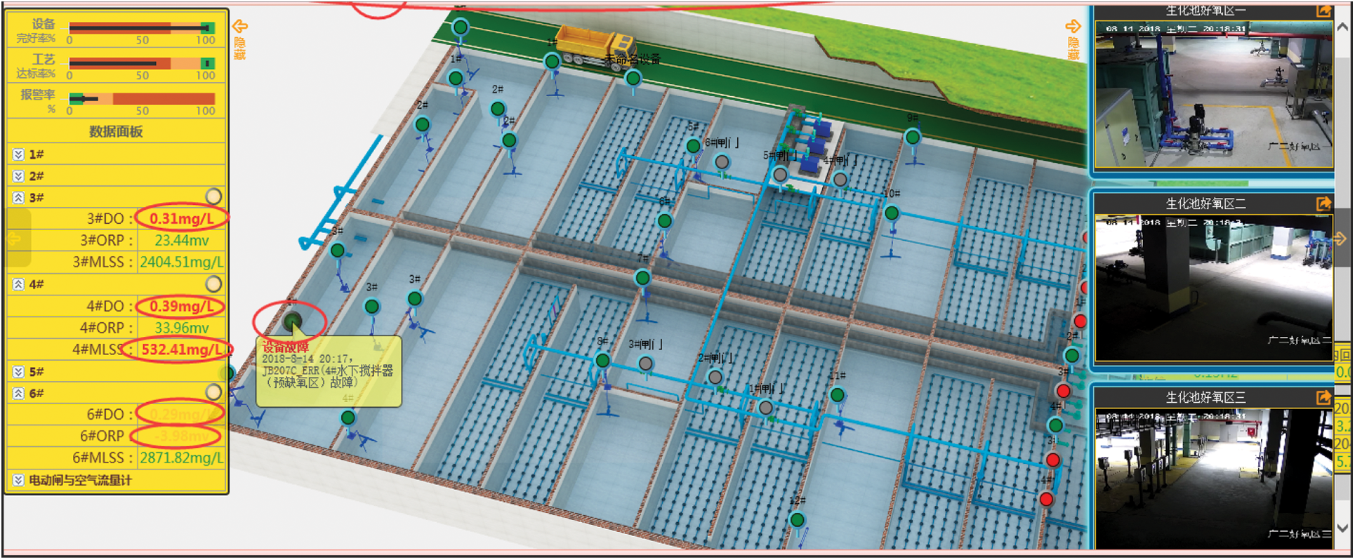
Figure 1: The interface diagram of the monitoring system platform

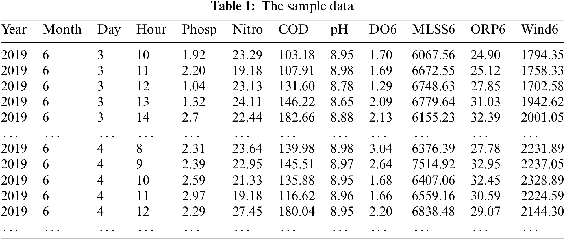
The data are collected hourly and in real-time display on the monitoring system platform. There are 8760 pieces of data a year for each variable collected. The data variables studied include “Year,” “Month,” “Day,” “Hour,” “Phosp,” “Nitro,” “COD (Chemical Oxygen Demand),” “pH,” “DO (Dissolved Oxygen),” “MLSS (Mixed Liquid Suspended Solids),” “ORP (Oxidation Reduction Potential),” and “Wind.” The four variables of “DO,” “MLSS,” “ORP,” and “Wind” in the biochemical pool have six sampling points, respectively, so each process parameter variable has six values, such as “Wind1,” “Wind2,” … and “Wind6.”

The sample data is shown in Table 1. In Table 1, the “Phosp” indicates total phosphorus, “Nitro” means water ammonia nitrogen, and “Wind” indicate wind speed.

3.1.2 Feature Selection Based on Random Forests

The random forest approach is based on a decision tree “bagging” algorithm. Use “bagging” methods to train a single individual into multiple training troops. A decision tree is constructed for each training set to transform the single decision tree model into a multi-decision tree model. Finally, the average value of the multi-decision tree is obtained. The random forest approach can integrate new theories to face different application scenarios to improve performance. Many experiments have tested the performance of the random forest approach in feature selection. For example, Wong et al. [20] establish the energy consumption prediction model using the random forest feature selection algorithm. Compared with the single machine learning algorithm, the prediction performance of the subset selected by random forest features as input has been dramatically improved. Wang et al. [21] mention that random forest features were used to screen woodland classification. The results showed that the classification accuracy of the established model after screening features was nearly 10% higher than that of the original parts. Lai et al. [22] mention that the experiment shows that the prediction accuracy of red tide grade can be higher than other methods by using the selected subset of random forest features. Choosing a random forest as a feature selection method is applicable.

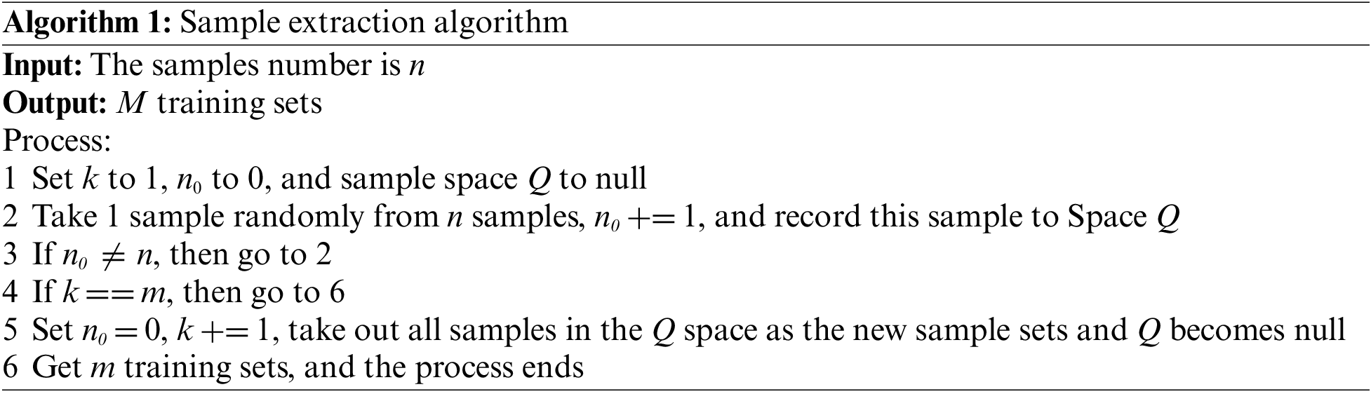
With only one training set and n sample sizes, training M sets of the same size are now required. The principle of the “bagging” algorithm is to extract one of the sample data from N samples randomly. Record and put it back, go back and forth N times, and arrive at a new training set with N samples. Repeat M times in the above procedure to get the M sample sets with N samples that meet your needs. With M training sets, each training set is modeled separately, not directly related to each other, and finally, the M models are consolidated to get the final result. Initializes the sample set k to 1, the sample size n to 0. There are n samples in the sample set, which requires M training sets. The algorithm is shown as follows Algorithm 1.

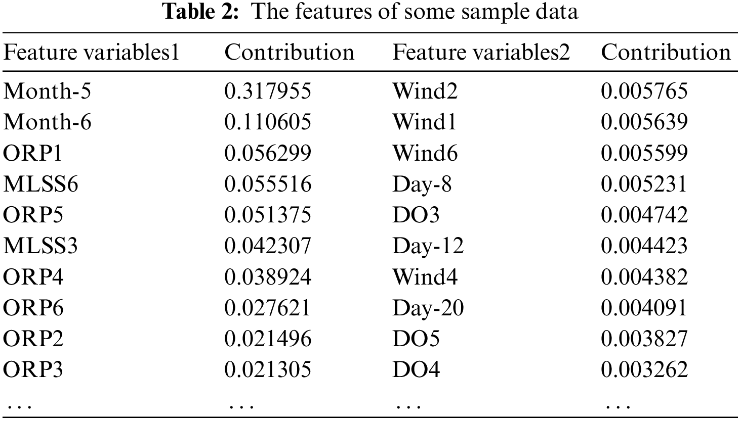
The random forest method is used for feature selection. The month, day, and time variables in the data source with time features are coded conversion as 0/1 classified variables and are replaced into random forest algorithms to select features. Use contribution to evaluate the feature variable’s importance, set the feature variables whose contribution is more than 0.001, and sort as a subset of features. Some of the results are shown in Table 2.

3.1.3 Standardized Processing of Data

It can be found that the data range varies considerably. For example, the “DO” ranges from about 1 to 10, while the “MLSS” value ranges from 3000 to 8000. Suppose these data are put directly into the model to train. In that case, it will result in a more significant role for features with large numbers and a feature with a smaller number to play a minor role in modeling, which is not common sense, so the data must be standardized. All features must be uniformly scaled to have the same degree of influence when the gradient drop method is used. This processing is a prerequisite for the successful establishment of a prediction model.

Data standardization methods typically use the min-max standardized method, also known as the unification method, which converts the raw data into the interval of [0, 1] by the Eq. (1). Where y is normalized data, x is raw data.

yi=xi−min1≤j≤n{xj}max1≤i≤n{xj}−min1≤i≤n{xj}(1)

3.2 Deep Learning Model Construction

The CNN model structure combines convolutional correlation calculation and deep BP (Back Propagation) neural network. The feature extraction of original samples is carried out using convolution in the convolution layer. The convolution process is shown in Fig. 2.

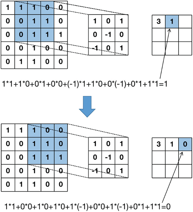
Figure 2: The convolution computation procedure

CNN is a model composed of three steps: convolution, pooling, and activation function. After the convolution calculation step, pooling is used to reduce the dimension of the previous step’s result data and expand the field of vision. The activation function is added to make the neural network more excellent in simulating nonlinear factors. The CNN model constructed in this study is shown in Fig. 3. Finally, the fully connected neural network layer is used to nonlinearly combine the previous step’s output to get the target demand classification or regression.

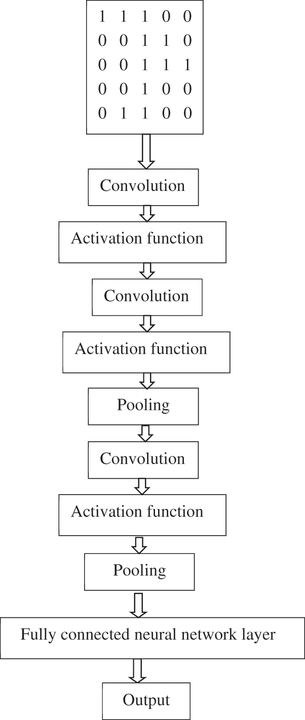
Figure 3: The CNN model constructed

Using the feature of convolution, CNN has the following advantages [23]:

•   The feature has translation invariance. When extracting features, convolution will integrate the complete information after the convolution calculation of each local knowledge so that it will retain the feature information of the original two-dimensional grid space. So the feature after input extraction has translation invariance, which is challenging to maintain on the traditional neural network.

•   When feature extraction is carried out, continuous local data will be convolved, and the results will be generated along with the sliding calculation of the convolution kernel. However, in the traditional neural network, features are used as the partition for weight calculation.

•   The values in the convolution kernel are always constant when the local space is convolved by sliding convolution. From the perspective of each local space that keeps sliding, their convolution kernel weights are shared. After the result is obtained, each value only has a connection relation with the original local space and convolution kernel and has no association with other local spaces of the original two-dimensional grid. Such a connection is called a sparse connection. The benefits of this feature are enormous.

3.3 Wastewater’s pH Modeling

3.3.1 The Algorithm of Modeling

Firstly, the original sample set is featured, and the processed subset of the sample is then converted through a sliding window [24], processing to time series and input into the CNN model for training. CNN’s internal model contains convolution layers and pooled layers. A convolution layer of 2 layers can reduce the output dimension relative to one pooled layer alternately. Each layer of operations requires nonlinear activation operation processing. After the end of the alternating combination, all features are output into the fully connected neural network for subsequent operations. Finally, the connection output of the full-connection layer is handled by dropout to prevent the model from overfitting. The entire model will use the Adam optimization algorithm and loss function to train to produce the final results.

The algorithm for building the model is as follows Algorithm 2.

3.3.2 The Sliding Windows

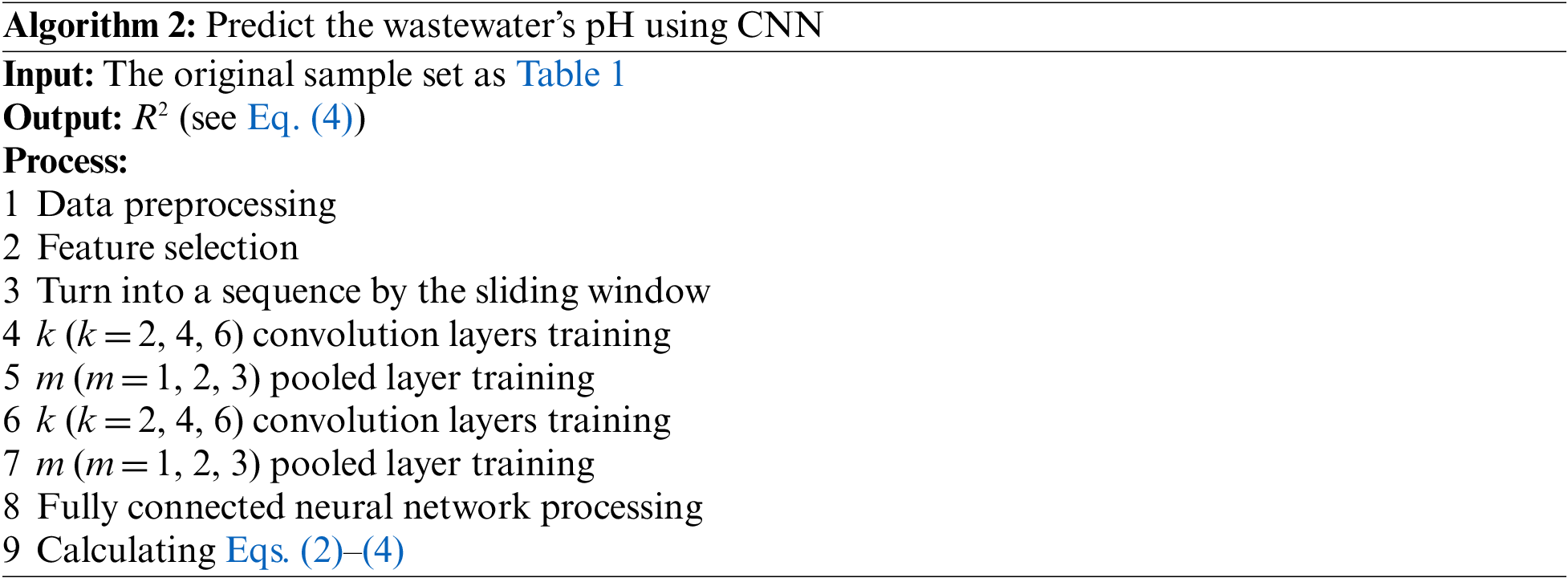
Before training a prediction model using CNN, the research must convert the input sample data to timing data for subsequent operations. In order to ensure the prediction effect of the CNN model, the sliding window method is added to the model in this study, which can dynamically use the latest data subset. This method is used in many studies. For example, Mishra et al. [25] addresses the disaster data updates in different periods, and a dynamic, optimized model with a sliding time window is proposed.

The operations of converting to timing data are as follows:

(1)   Select the sliding window, the time interval for which is n in size.

(2)   Slide all variables in the sample set chronologically, starting with the first sample. The matrix of n samples in the sliding window is treated as one sample entered for subsequent CNN modeling.

(3)   Until the last sample in the original sample is filtered by a sliding window, it is considered the previous sample of the CNN modeling input, and a new time series input is formed.

The flowchart of the sliding window is as Fig. 4 below, each number represents the nth row sample in the original sample set, and each row of pieces is multivariable. With a sliding window size of 4, the first to the fourth sample is taken as a new input sample. With the sliding window to the right moving, the new input matrix will also increase as the sliding window moves until the last piece is included to form a new one-dimensional time series input. It is crucial to observe the effect of different time window sizes on the experimental results for sliding windows. Fan et al. [26] points out that the scientific determination of the optimal sliding window size is significant research work. In the experiment, the time interval sizes will be divided into 8, 12, and 15 to form a new time series input source. Then, make prediction modeling separately to see how much the sliding window sizes can get better results.

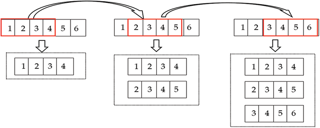
Figure 4: The flowchart of the sliding window

4  Results and Discussion

4.1 Experimental Method

For processing time series, CNN can handle the relationship between the sample of multi-dimensional well because of its convolutional features, thereby increasing predictive accuracy. The nonlinear activation function is used in each layer of operations in CNN to fit the nonlinear relationship between multi-dimensional variables in wastewater treatment. The last and full-connection layers can further improve the model’s accuracy. Finally, compared to fully connected neural networks, CNN based on sliding windows has the features of local sensation, weight sharing, and sparse connectivity, which makes CNN’s time complexity in model training much less than that of a fully connected neural network. Therefore, converting the input to time series using CNN to make relevant predictions is feasible. While sliding window processing, convert the feature subset to a time series with 8, 12, and 15 sample data as a time interval, respectively. The experimental process is as follows:

(1)   Set the interval size based on the sliding window to 8, 12, and 15, respectively. Then generate six-time series input sources with time-characteristic data sources in three sliding window interval sizes.

(2)   CNN will then use three models for comparative training: 2-tier convolution and 1-tier pooling; 4-tier convolution and 2-tier pooling; 6-tier convolution and 3-tier pooling. The pooled tier sizes are 2, and nonlinear activation is performed on each layer.

(3)   The research set the convolutional number to 32 and 64, respectively. To compare the results of the iteration, select the convolution kernel size of 3.

(4)   The full-connection layer is connected. The parameters of the full-connection layer are adjusted. The final results are output, and the entire model is trained.

When the entire data set is converted into a time series, the training and test groups are divided into 7:3 scales. The training set is input into the CNN model to be trained to produce a prediction model. Then the test set is input into the prediction model to produce the prediction results. Then the results are compared to the actual value. The training model will be used R2 indicators to assess the quality of the model prediction results with the parameters at this time to select which parameters can be built a better prediction model.

The R2 is a good representation of the fit of the predictive and accurate models. Set y as the actual value, y¯ is the average of all actual values, y^ is the prediction value, SSR is the regression square sum, and SST is the total square. Their calculations are as follows Eqs. (2)–(4).

SSR=∑i=1n⁡(y^i−y¯)2(2)

SST=∑i=1n⁡(yi−y¯)2(3)

R2=SSRSST=∑i=1n⁡(y^i−y¯)2∑i=1n⁡(yi−y¯)2(4)

The interval values of R2 are between 0 and 1. When the values are closer to 1, the better fit and the tighter the actual model. The closer it is to 0, the worse the model fits.

4.2 Experimental Results

Because the sliding window interval size is set to 8, 12, and 15, respectively, the experiments have been done with three sets of input data sources. Each set of experimental data sources is adjusted with a different convolutional number in the CNN model, and get the results of R2 at this time. Partial results are shown in Table 3.

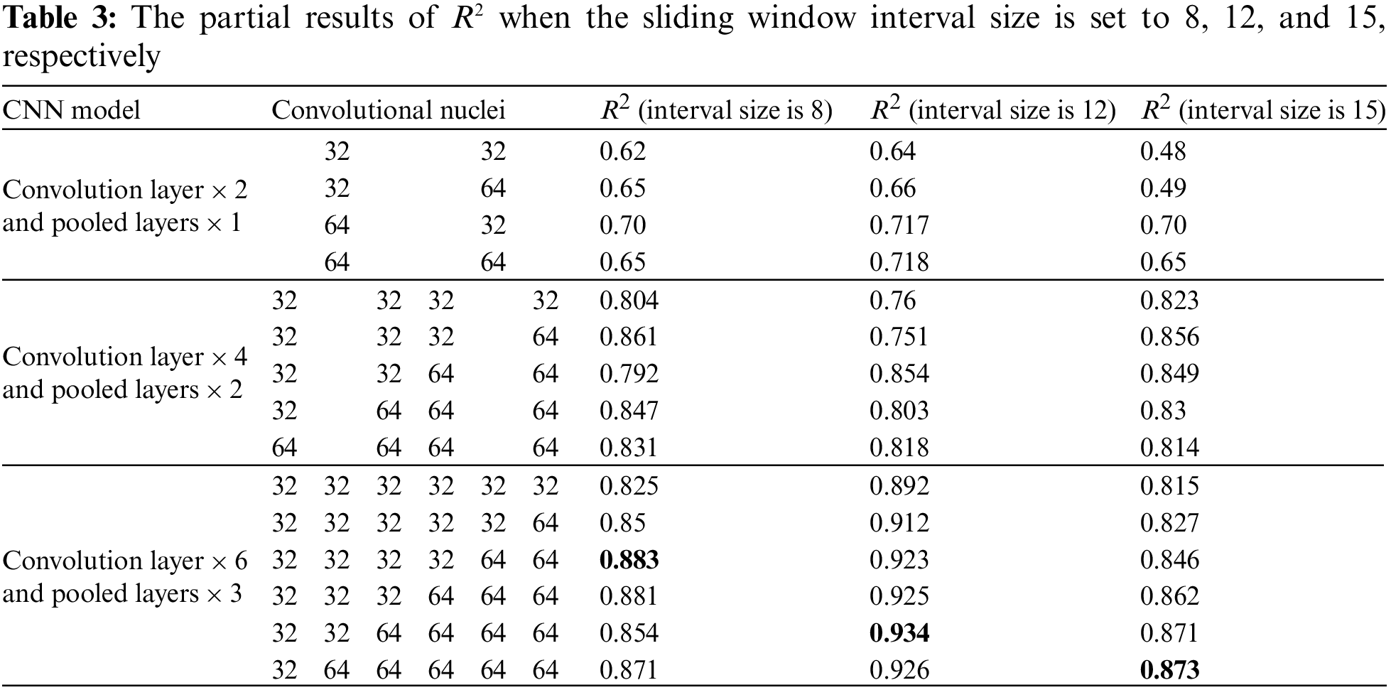
The experimental results in Table 3 show that the best fitting value was 0.883 when the time interval size of the input data source was eight and convolutional numbers were 32, 32, 32, 32, 64, and 64, respectively. The optimal fitting value was 0.934 when the time interval size of input data sources was 12 and convolution numbers were 32, 32, 64, 64, 64, and 64, respectively. The optimal fitting value was 0.873 when the time interval size of input data sources was 15, and convolutional numbers were 32, 64, 64, 64, 64, and 64, respectively. The better model for three sets of data sources is 6-tier convolution and 3-tier pooling layers.

After confirming the CNN structure, it can be connected to the full-connection layer to obtain the output results. The parameters of the full-connection layer can also be adjusted, mainly to regulate the number of neurons and the number of hidden layers. Because the precision of the fitting model in the convolution layer is high, the full-connection layer experiments only with 1 to 3 hidden layers. Because too high a hidden layer will lead to overfitting, choosing a higher number of hidden layers is unnecessary. The hidden node selection for each layer has experimented with 16 initial and two multiples to 64. The full-connection layer parameters are adjusted for each of the three sets of data sources, and each hidden node is at the same level. The partial results are shown in Table 4.

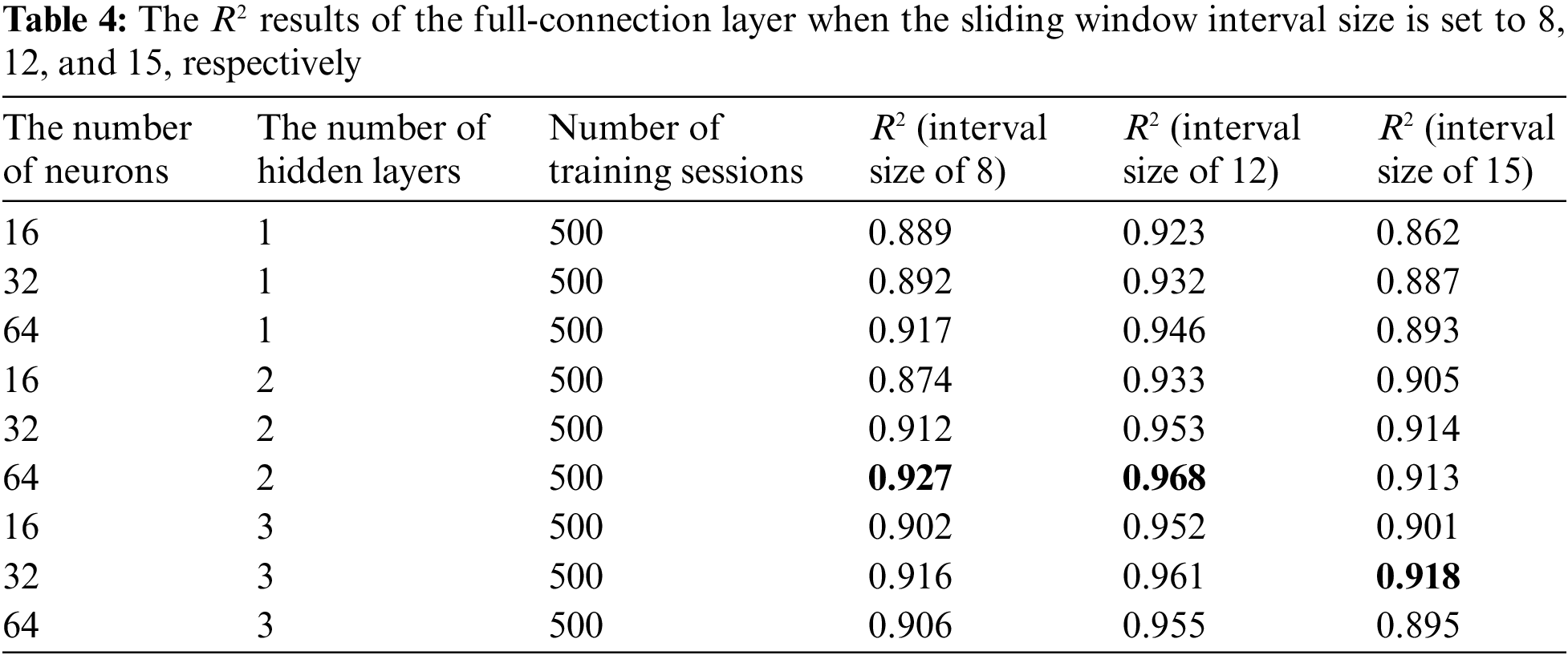
From the adjustment results of the full-connection layer, it can be seen that the R2 results of the input data source with a time interval size of 12 are significantly higher than that of the time interval size of 8 and 15. The model loss process functions trained by the three sets of data sources are shown in Fig. 5.

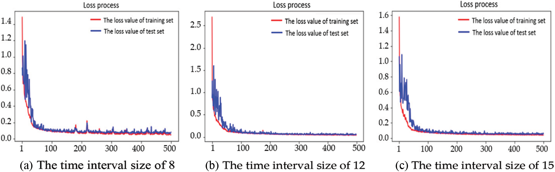
Figure 5: The loss process to model with different time interval sizes

The three sets of loss process function diagrams show that when the number of training times exceeds 300, the training set loss value and test set loss value are leveled off. Currently, the training model accuracy of the three sets is nearly optimal. The number of re-adjusting training is unnecessary. Therefore, only adjust the training times of the model established by the input data source with the time interval size of 12 to observe whether it can obtain better accuracy.

The iteration of the number of training starts at 300, gradually increasing the number of iterations by 100 training times to observe the fitting results. When the fitting degree has an increment and then a decrease, the fit has changed from underfitting to overfitting, and there is no need to continue to adjust the parameters. The result is shown in Fig. 6.

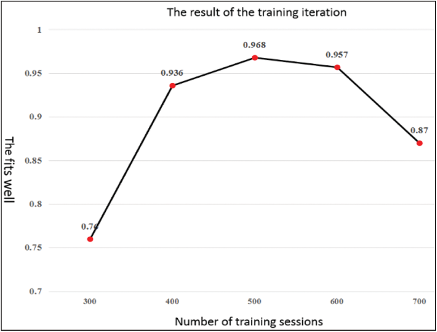
Figure 6: The iteration results of data source modeling training with a time interval size of 12

The results show that the optimal fit can be achieved when the number of training sessions is precisely equal to 500. Therefore, for data sources with a time interval size of 12, the optimal model is determined to use six convolutional layers and three pooled layers, with kernel numbers of 32, 32, 64, 64, 64, and 2 fully connected layers with 64 neurons per layer. The training times are 500, and the fitting degree is 0.968.

The fit of the actual and predicted values from three different data sources with varying intervals of time are shown in Fig. 7. The fit in Fig. 7b is better, and the curve of the actual and predicted values is the closest. Under normal circumstances, the wastewater’s pH is between 6.5 and 8.5, and the optimal value is around 7.4. It can be seen from Fig. 7 that the predicted pH of the sewage is between 7.2 and 8.6, so the prediction result is feasible.

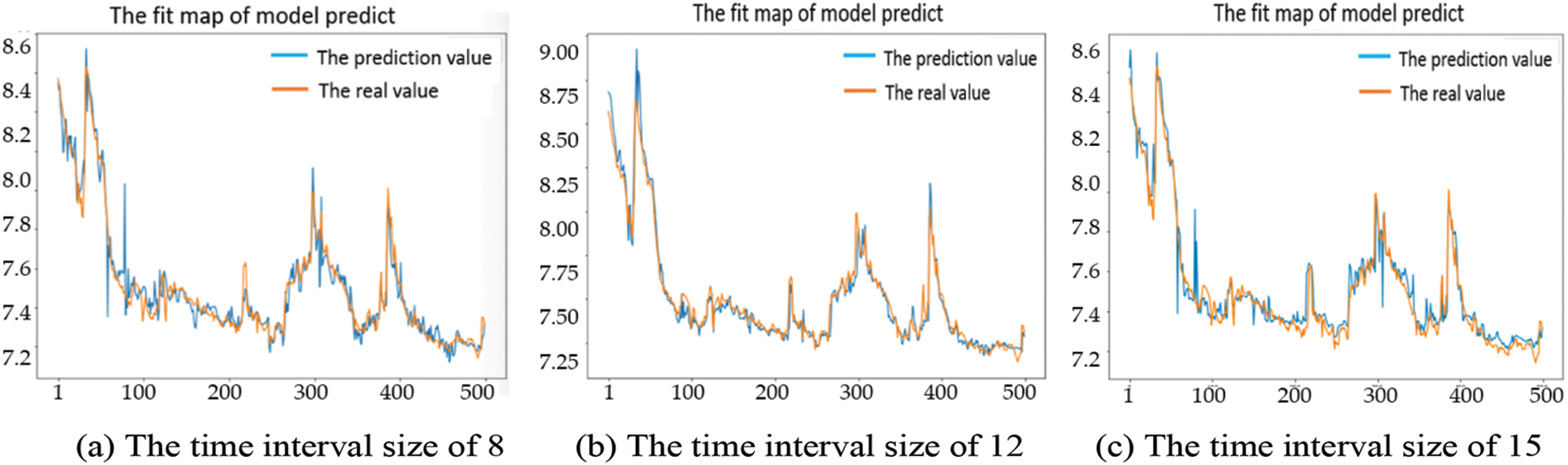
Figure 7: The loss process to model with different time interval sizes

4.3 Analysis of Results

Three data sources have been experimented with to produce a better model. Table 5 shows that for data sources with a time interval size of 8, determine a model with a 6-tier convolution layer and a 3-tier pooled layer. The convolutional number are 32, 32, 32, 32, 64, 64, the optimal model contains a full-connection layer with two layers and 64 neurons per layer, which needs 500 training sessions, and the fitting degree is 0.927. For data sources with a time interval size is 15, determine that a model with a 6-tier convolution layer, a 3-tier pooled layer. The convolutional number 32, 64, 64, 64, 64, 64, the optimal model contains a full-connection layer with three layers and 32 neurons per layer, which needs 500 training sessions, and the fitting degree is 0.918. For data sources with a time interval size of 12, determine that a model with a 6-tier convolution layer, 3-tier pooled layer, and the convolutional number are 32, 32, 64, 64, 64, 64. The result is that a full-connection layer with two layers and 64 neurons per layer is the optimal model, which needs 500 training sessions, and the fitting is 0.968.

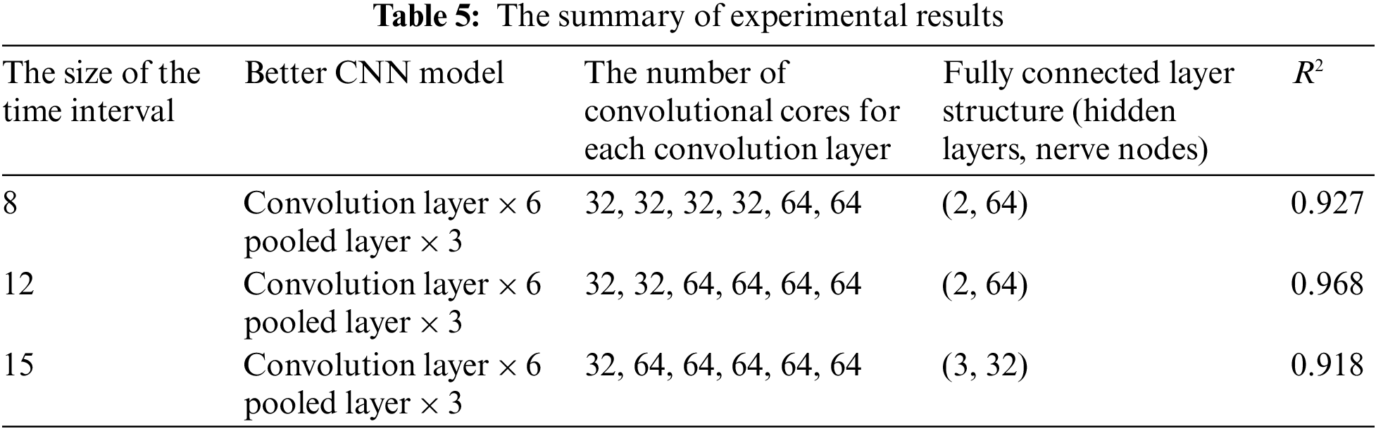
The better-trained CNN model in Table 5 contains six convolution layers and three layers of pooled layers, and the model was built by data sources with a time interval size of 12. Followed by a data source with a time interval size of 8, the worst fit compared to the 1st and 2nd groups is the model trained by a data source with a time interval size of 15. The model accuracy trained by data sources in different time intervals indirectly indicates that the sample data contain periodic patterns. Samples are built in unit hours, and models made in time series with a time interval of 8 are not as good as sequential models with 12. This indicates that sample data observed every 8 h is less regular than observed every 12 h.

4.4 Application of the Research Results

The result of the research in this paper is applied in the monitoring system platform of the “intelligent operation and maintenance platform of reclaimed water plant" (See 3.1.1 for a brief description of the project). The pH value of outgoing wastewater describes the degree of acidity and alkalinity of an aqueous solution. The aqueous solution with pH = 7 is neutral. It can be seen from Fig. 8 that the pH of incoming wastewater deviates from 7, but the pH of outgoing wastewater is around 7. The project’s practical application results show the research result’s feasibility.

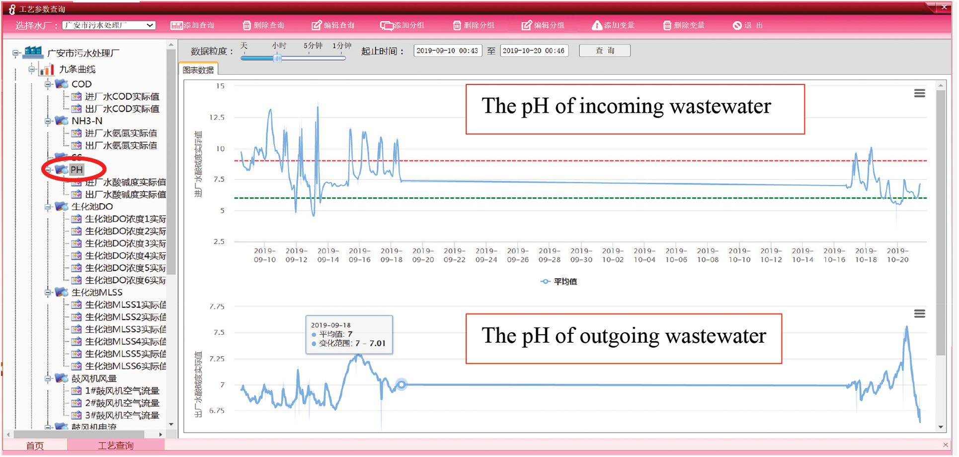
Figure 8: The pH of incoming wastewater and outgoing wastewater in the application platform

5  Conclusions

This study establishes the deep learning model through historical data analysis to ensure that the wastewater’s pH of the sewage treatment plant is within the emission standard range. Firstly, multiple variables are selected, such as in Table 1. The features of the data are determined by the embedded random forest method. The feature subset data source is the input of the deep learning model. In deep learning model training, the slide window method is adopted. Since the size of the sliding window directly affects the prediction effect of the model, a lot of experiments on the selection of the sliding window size are done in this study. The results show a better evaluation value can be obtained when the sliding window size is 12.

On the other hand, the selection of the number of convolution layers and pooling layer in the deep learning model is also tested by different choices. The results show that better prediction results can be obtained when the convolution layer is six and the pooling layer is three. Finally, the deep learning training model predicts the wastewater’s pH. The real value and the prediction value are compared. The comparison results show that when the convolution layer is selected for six, the pooling layer is chosen for 3, the full-connection layer with two layers and 64 neurons per layer, and the sliding window size is selected for 12, the results are better. The research deep learning model has a good application effect in practical application.

The wastewater’s pH is one of the indicators of wastewater quality, and the modeling of each indicator is different. Limited by space, this paper only studies the deep-learning modeling of wastewater’s pH. Later, it will further explore the modeling of other wastewater indicators and seek more advanced deep-learning models.

Acknowledgement: The authors would like to thank the editor and the anonymous reviewer whose constructive comments will help improve this paper’s presentation.

Funding Statement: This research was funded by the National Key R&D Program of China (No. 2018YFB2100603), the Key R&D Program of Hubei Province (No. 2022BAA048), the National Natural Science Foundation of China program (No. 41890822) and the Open Fund of National Engineering Research Centre for Geographic Information System, China University of Geosciences, Wuhan 430074, China (No. 2022KFJJ07). The numerical calculations in this paper have been done on the supercomputing system in the Supercomputing Centre of Wuhan University.

Conflicts of Interest: The authors declare that they have no conflicts of interest to report regarding the present study.

References

1. S. M. Lencha, M. D. Ulsido and A. Muluneh, “Evaluation of seasonal and spatial variations in water quality and identification of potential sources of pollution using multivariate statistical techniques for lake hawassa watershed, Ethiopia,” Applied Sciences, vol. 11, no. 9, pp. 8991, 2021. [Google Scholar]

2. X. A. Wang, Q. Cao and X. Shi, “Progress in research on sewage treatment at home and abroad,” Applied Chemical Industry, vol. 51, no. 1, pp. 176–182, 2021. [Google Scholar]

3. A. Szarka, V. Mihová, G. Horváth and S. Hrouzková, “Development of an advanced inspection of the degradation of volatile organic compounds in electrochemical water treatment of paint-industrial water effluents,” Applied Sciences, vol. 13, no. 1, pp. 443, 2023. [Google Scholar]

4. F. Kristjanpoller, N. Cárdenas-Pantoja, P. Viveros and R. Mena, “Criticality analysis based on reliability and failure propagation effect for a complex wastewater treatment plant,” Applied Sciences, vol. 11, no. 22, pp. 10836, 2021. [Google Scholar]

5. H. G. Han, S. H. Yang, L. Zhang and J. Qiao, “Optimal control of effluent ammonia nitrogen for municipal wastewater treatment process,” Journal of Shanghai Jiao Tong University, vol. 54, no. 9, pp. 916–923, 2020. [Google Scholar]

6. M. Aamir, Z. Li, S. Bazai, R. A. Wagan, U. A. Bhatti et al., “Spatiotemporal change of air-quality patterns in Hubei province-a pre- to post-COVID-19 analysis using path analysis and regression,” Atmosphere, vol. 12, pp. 1338, 2021. [Google Scholar]

7. N. Ahmed, A. L. C. Barczak, S. U. Bazai, T. Susnjak and M. A. Rashid, “Performance analysis of multi-node hadoop cluster based on large data sets,” in 2020 IEEE Asia-Pacific Conf. on Computer Science and Data Engineering, Gold Coast, Australia, pp. 1–6, 2020. [Google Scholar]

8. P. T. Shi, J. D. Wang and J. H. Wang, “Research on modeling of wastewater treatment process based on hybrid model,” Computer Simulation, vol. 37, no. 8, pp. 188–191, 2020. [Google Scholar]

9. Z. Q. Li, J. Q. Du, B. Nie, W. P. Xiong, C. Y. Huang et al., “Summary of feature selection methods,” Computer Engineering and Applications, vol. 55, no. 24, pp. 10–19, 2019. [Google Scholar]

10. Z. H. Zhao, Z. H. Wang, J. L. Yuan, J. Ma, Z. L. He et al., “Development of a novel feedforward neural network model based on controllable parameters for predicting effluent total nitrogen,” Engineering, vol. 7, pp. 195–202, 2021. [Google Scholar]

11. L. Zhang, J. C. Zhang, H. G. Han and J. F. Qiao, “FNN-based process control for biochemical phosphorus in WWTP,” CIESC Journal, vol. 71, no. 3, pp. 1217–1225, 2020. [Google Scholar]

12. L. Chen, “Foreign exchange rates forecasting with convolutional neural network,” M.S. Dissertation, Zhengzhou University, Zhengzhou, China, 2018. [Google Scholar]

13. H. Nan, L. Lu, X. J. Ma, Z. D. Hou, C. Zhang et al., “Application of sliding window algorithm with convolutional neural network in high-resolution electron microscope image,” Journal of Chinese Electron Microscopy Society, vol. 48, no. 3, pp. 242–249, 2021. [Google Scholar]

14. O. Abdel-Hamid, A. R. Mohamed, H. Jiang, L. Deng, G. Penn et al., “Convolutional neural networks for speech recognition,” IEEE/ACM Transactions on Audio, Speech, and Language Processing, vol. 22, no. 10, pp. 1533–1545, 2014. [Google Scholar]

15. S. Liu, H. Ji and M. C. Wan, “Nonpolling convolutional neural network forecasting for seasonal time series with trends,” IEEE Transactions on Neural Networks and Learning Systems, vol. 31, no. 8, pp. 2879–2887, 2020. [Google Scholar] [PubMed]

16. Y. F. Lin, Y. Y. Kang, H. Y. Wan, L. Wu and Y. X. Zhang, “Deep spatial-temporal convolutional networks for flight requirements prediction,” Journal of Beijing Jiaotong University, vol. 42, no. 2, pp. 1–8, 2018. [Google Scholar]

17. W. W. Tan, J. J. Zhang, J. Wu, H. Lan, X. Liu et al., “Application of CNN and long short-term memory network in water quality predicting,” Intelligent Automation & Soft Computing, vol. 34, no. 3, pp. 1943–1958, 2022. [Google Scholar]

18. X. K. Zhan, “Research on time series forecasting methods based on time convolution and long short-term memory network,” Ph.D. Dissertation, Huazhong University of Science and Technology, Wuhan, China, 2018. [Google Scholar]

19. B. Meriem and O. Jamal, “Multivariate time series forecasting with dilated residual convolutional neural networks for urban air quality prediction,” Arabian Journal for Science and Engineering, vol. 46, pp. 3423–3442, 2021. [Google Scholar]

20. W. Y. Wong, A. K. I. Al-Ani, K. Hasikin, A. S. M. Khairuddin, S. A. Razak et al., “Water quality index using modified random forest technique: Assessing novel input features,” Computer Modeling in Engineering & Sciences, vol. 132, no. 3, pp. 1011–1038, 2022. [Google Scholar]

21. X. F. Wang, “Study on forest classification based on random forest algorithm,” Forestry Science and Technology, vol. 46, no. 2, pp. 34–37, 2021. [Google Scholar]

22. X. Y. Lai, Q. D. Zhu, H. R. Chen, Z. Wang and P. J. Chen, “Red tide level prediction based on RF feature selection and XGBoost model,” Journal of Fisheries Research, vol. 43, no. 1, pp. 1–12, 2021. [Google Scholar]

23. Y. J. Li, T. Zhang, C. H. Dan and Z. Y. Liu, Deep Learning: Mastering Convolutional Neural Networks from Beginner, 1st ed. Beijing, China: China Machine Press, pp. 20–75, 2018. [Google Scholar]

24. W. Tang, S. C. Ma and C. Li, “LSTM ground temperature prediction method based on sliding window,” Journal of Cheng Du University of Technology (Science and Technology Edition), vol. 48, no. 3, pp. 377–383, 2021. [Google Scholar]

25. B. K. Mishra, K. Dahal and Z. Pervez, “Dynamic relief items distribution model with sliding time window in the post-disaster environment,” Applied Sciences, vol. 12, no. 16, pp. 8358, 2022. [Google Scholar]

26. Z. Y. Fan, H. Y. Feng, J. G. Jiang, C. G. Zhao, N. Jiang et al., “Monte carlo optimization for sliding window size in dixon quality control of environmental monitoring time series data,” Applied Sciences, vol. 10, no. 5, pp. 1876, 2020. [Google Scholar]