A Spatio-Temporal Heterogeneity Data Accuracy Detection Method Fused by GCN and TCN

1  Introduction

Spatio-temporal heterogeneity data (STD) [1–3] is the data basis for applying big data analysis technology to solve decision-making problems in urban operation and maintenance [4], oil and gas development [5], medical decision-making [6], life sciences [7] and other fields, and its accuracy detection is undoubtedly important [8,9]. Due to the stochasticity and complexity of STD in the temporal dimension and the global and local correlation in the spatial dimension, which makes detection extremely difficult, related research has also become a research hotspot for data analysts [10]. The current STD Accuracy Detection Method (SAM) mostly uses rule-matching algorithms based on expert experience, for example, network traffic detection [11,12], land classification management [13], and behavior pattern monitoring [14]. Although it is possible to screen out anomalous data to some extent, the following problems remain. On the one hand, the reliability of some experts’ experience has not been checked, leading to possible errors in the test results. On the other hand, it is difficult for experts to cover all the rules, which makes some anomalous data become to slip through the net, especially logical errors that do not satisfy the spatiotemporal correlation of data and are often overlooked.

With the rapid development of artificial intelligence, deep learning technology has roared in the field of data quality control with its powerful spatiotemporal data analysis capability, the key techniques include graph convolutional networks and temporal convolutional networks. Based on graph theory, Graph Convolutional Networks (GCN) [15–17] uses Fourier transform and Convolution Theorem to capture the spatial dependence of data objects, and thus implement data detection. Therefore, it is suitable for application scenarios containing spatial information such as action recognition [18] and image classification [19]. In the paper [20] presents a novel intelligent system based on graph convolutional neural networks to study road crack detection in intelligent transportation systems. In the paper [21], a group behavior pattern recognition algorithm based on spatiotemporal graph convolutional network is proposed, aiming at group density analysis and group behavior recognition in video. However, since the graph itself cannot reflect the time-varying, the GCN is not suitable for the accurate detection of time series data. Temporal Convolutional Networks (TCN) use Dilated Causal Convolutions and residual connectivity to extract temporal features of the data [22–24], which can effectively solve the problem of accurate detection of log data [25] and network data [26]. In the paper [27], a time-convolutional network (TCN)-based spectrum sensing method is designed, which improves the detection probability by using temporal features to enhance the spectrum sensing performance. In this paper [28], a denoising temporal convolutional recurrent autoencoder (DTCRAE) is proposed to improve the performance of the temporal convolutional network (TCN) on time series classification (TSC). However, it is difficult to solve the accuracy detection problem of data with spatial characteristics because it cannot describe space variation.

Therefore, this article proposes a method to detect the accuracy of spatiotemporal heterogeneous data by fusing graph convolution and temporal convolution networks, based on the hybrid intelligent algorithm design idea of “divide and conquer, complementary advantages” [29,30]. Firstly, the geographic weighting function is introduced and improved to quantify the degree of association between nodes and calculate the weighted adjacency value, thus achieving the purpose of simplifying the complex topology. Secondly, the spatiotemporal convolution unit is designed based on the graphical convolutional neural network and temporal convolutional network, while the temporal activation function is optimized to improve the detection speed and detection accuracy. Finally, this article designs a series of comparative experiments in real application scenarios to verify that this method has obvious advantages in terms of detection speed and detection accuracy.

The innovations in this article include:

1. This article fuses GCN and TCN to solve the problem of feature extraction and analysis for spatiotemporal heterogeneous data.

2. This article proposes an adaptive geographically weighted function for enhancing the saliency of model spatial feature extraction. At the same time, the activation function of the temporal convolutional network is optimized to avoid the overfitting of the network, which in turn enhances the generalization ability of the network.

The method proposed in this article has a good application effect in many real-world scenarios. For example, while checking data quality with its data interchange platform, the Research Institute of an Oilfield Co., Ltd., chose this method to check data accuracy. In the actual application, this method has a faster run time, and the accuracy is superior to the original method. Thus, it saves considerable time and economic cost for the scientific research institution and greatly promotes the information management of the oilfield.

The structure of this article is shown below. Section 2 gives the application scenarios, describes the basic concept and formula, and generalizes the key problems. Section 3 expounds on how to deal with complex topology structures. Section 4 elaborates on the operation mechanism and improvement points of FAGTN. Section 5 verifies the validity of the method. Section 6 summarizes the study and prospects for future work.

2  Fundamental Work

This section gives the definition of the scenario and the basic concepts and described the key problems to be solved.

2.1 Scenarios and Basic Concepts

Define scenario H: In the spatiotemporal heterogeneity environment composed of n data objects (nodes), the data center released a group of spatiotemporal heterogeneity data accuracy testing tasks B, and the number of tasks is Z. Any one task is Bm∈B is composed of n nodes and will be solved by an intelligent data detection method. The intelligent data detection method includes 2 stages. Stage1 calculates and filters weighted adjacency values. The complex topologies of the detected space are pruned. Stage 2 Performs data detection based on GCN and TCN (“FAGTN”), and construct the temporal and spatial features analysis model, as shown in Fig. 1. Any node of Bm can be expressed as Bmk=(Lk,A,T,X), Lk denotes the spatial location of a node vk, A∈Rn×n means the spatial adjacency relationship between nodes, T indicates the time, and X represents the set of attribute values for the node at time T.

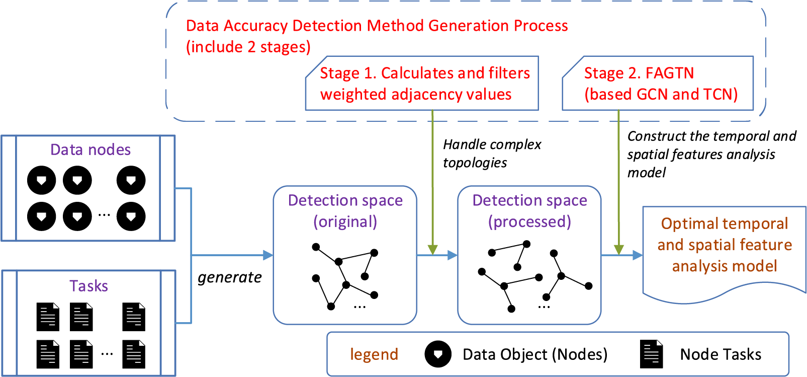
Figure 1: Work process of FAGTN

Since the given task is advanced detection of data, the node attributes in scenario H have integrity and satisfy the following three preconditions.

Precondition 1. Common attributes exist for all nodes in the same task, and the attribute value is not null.

Precondition 2. The adjacency matrix of a node cannot be an identity matrix, that is, A≠IN×N.

Precondition 3. Due to the complexity of node relationships, this article constrain the node’s adjacency relationship to be non-transitive. For example, if v1 is connected to v2, v1 is connected to v3, and v2 is not connected to v3, then it is decided that v1 and v2 are adjacent, v1 and v3 are adjacent, but v2 and v3 are not adjacent.

The basic concepts, formulas, and reasoning processes can be described as follows.

I. Property Matrix. This article divides the time T into m time units, that is, T={t1,t2,…,tm}. The property matrix X represents the attribute values of n node in m time units under the current task. Xvitj represents the attribute value of node vi in time unit tj. Then the property matrix can be expressed as follows.

X=[Xv1t1Xv1t2⋯Xv1tmXv2t1Xv2t2⋯Xv2tm⋮⋮⋯⋮Xvnt1Xvnt1⋯Xvntm](1)

II. Weighted Adjacency Value. This article defines that λij represents the weight coefficient for nodes vi and vj, dij denotes the distance between vi and vj. The weighted adjacency value Aij∗ can be expressed according to “Weighted Adjacency Value = Weight Coefficient Distance”.

Aij∗=λij⋅dij(2)

III. Detection Space. In the target area G, any possible detection space Se(Se⊆G) consists of indeterminate nodes and satisfies the following constraints.

Constraint 1. Any detection space contains at least two nodes (derived from Precondition 2), and the number of nodes shall not be greater than n.

Constraint 2. Each node can appear in multiple detection spaces, but the nodes appearing under the same detection space must satisfy Precondition 3.

This article randomly selects a detection space S1, and assumes that this detection space is centered on v1 and contains all nodes adjacent to it v1. Thus, in the target area G, the number of detection spaces that may be formed can be expressed as follows. With the increase of node number and node degree, the number of detection spaces increases rapidly.

e=∑i=1n⁡∑p=1n⁡∑q=1n⁡Apqi(3)

2.2 Problem Description

The “optimal” spatiotemporal data detection model means as much as possible to meet the shortest time and best results. Shortest time means the shortest possible detection time and can be expressed as min(g(Se)), g(Se) representing the time objective function. The value g(Se) of depends on the number of detection spaces in a task and the time consumed by each detection space, which can be described as formula (4). Wherein, t(Se) stands for the detection time of the detection space Se, teAepθ represents the processing time of (ve,vp), θ is the training parameter.

min(g(Se))=min(∑e⋅t(Se))=min(∑θe⋅∑p=1n⁡teAep)(4)

Best results mean “the most accurate possible detection result”, which is reflected in giving accurate nodes’ attribute reference values at the current moment. Xvitj represents the attribute value of the child node vi in a time unit tj. The time series Tvi of child nodes vi can be expressed as {Xvit1,Xvit2,…,Xvitm}. The spatiotemporal sequence of the target detection task can be represented as {Tv1,Tv2,…,Tvn}. The value Xvit+1 depends on the historical attribute values of the detection space centered on this node. Therefore, this article can establish the mapping relationship f(A,X) between historical attribute values and reference values, which can be described as formula (5).

Xvit+1=f(A,X)=f{(Ai1∗Ai1Ai2∗Ai2⋮Ain∗Ain)T ,(Xvit1Xvit2⋮Xvitm)}(5)

In the end, the data accuracy detection problem can be described as the optimizing problem with min(g(Se)) and f(A,X) as the objective functions, and all objective functions are expected to obtain the best value.

This article collectively refers to node regions with prominent spatiotemporal heterogeneity as complex topology structure regions, and the more obvious such structural features are, the lower model processing speed and accuracy will be. Therefore, this article can preprocess the complex topology structure to improve the detection speed and detection accuracy.

In summary, the problems solved in this article can be described below.

I. How to handle the complex topology structure.

II. How to establish an excellent mapping relationship between historical attribute values and reference values in an environment with prominent spatiotemporal heterogeneity.

3  Handling Complex Topology Structure

Based on the definition of complex topology structure in the 2.2 problem description, this article introduces the concept of a graph to model the complex topology structure and uses the graph structure to describe the complex spatiotemporal relationships between nodes. The problem of “how to deal with complex topology structure” is transformed into “how to reflect the strength of node adjacency relationships in graph structure”.

3.1 Construction of Graph Model

To reflect the spatiotemporal heterogeneity of the data, this article designed a time-varying graph layer group with several depths, as shown in Fig. 2. Firstly, this article describes the spatial distribution of nodes with graphs, then stack the graphs according to time series, and finally store the task information of nodes as attribute features.

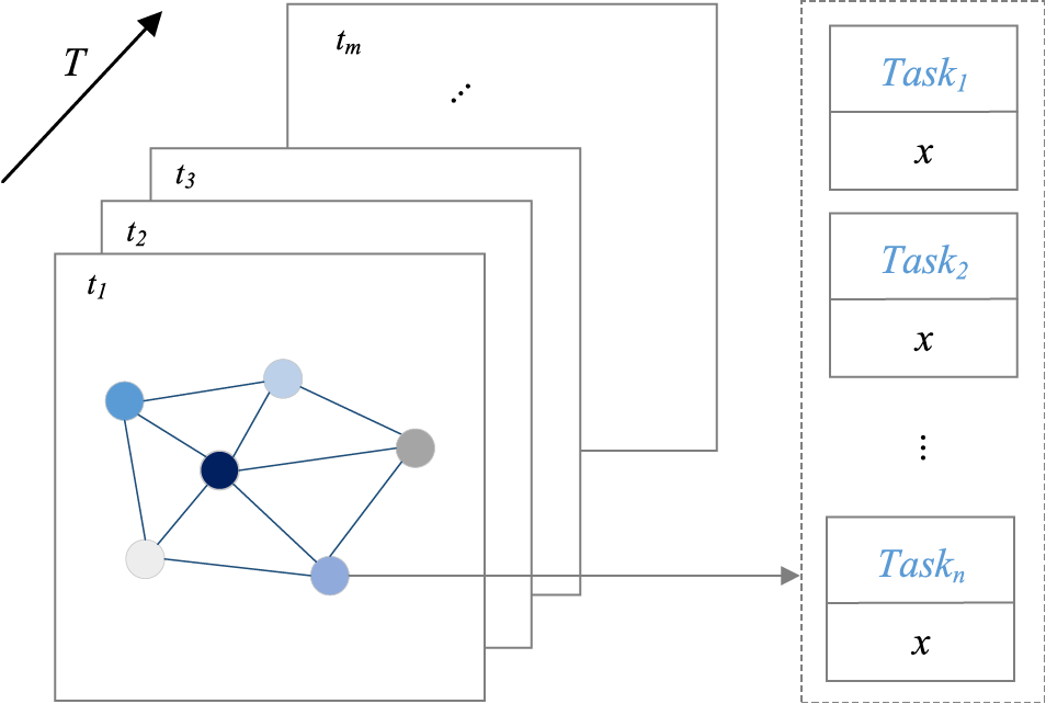
Figure 2: Overall design of time-varying graph layer groups

According to the 2.1 scenario description, this article defines the graph structure G(V,E,A,X), G describes all information about the nodes at a given time. V={v1,v2,…,vn} represents all nodes to be detected in the task, E={(vi,vj)|1≤i≤n,i≤j≤n,i≠j} means all edges that exist between nodes, A∈Rn×n indicates the adjacency matrix and X represents the property matrix for the node.

After modeling the scenario as a graph structure, this article calculates the weight coefficient among the nodes to achieve the operation of “weighting” [31,32]. On the whole, we achieve the effect that the sample points close to the center have more weight, otherwise the opposite. In the following, this article will discuss how to calculate the weight coefficient between nodes to describe the strength of the adjacency relationship.

3.2 Rules for Calculating the Weight Coefficient

This article usually uses the adjacency matrix to represent the connectivity between nodes. This article defines that Aij represents the adjacency value for nodes vi and vj, the value range and value condition Aij are shown in formula (6).

Aij={0,disconnected1,connected(6)

Formula (6) cannot reflect the strength of connectivity between nodes. This article proposes an adaptive geographically weighted function for nodes to determine the relationship between weights and distances, and the calculation rule is shown in Formula (7). Wherein, dij∗ stands for the Euclidean distance of nodes vi and vj, δ denotes the detection radius with the central node as the core. The function exhibits a monotonically decreasing trend, that is, the weight decreases as the distance increases.

λij=exp⁡(−(dij∗)22δ2)(7)

In the geographic weighting process, this article refers to the detection radius as the bandwidth, which is a trainable parameter whose magnitude affects the function’s slope. The time-varying layer group we built contains several detection spaces with different node locations and connectivity, which makes it impossible to use the same bandwidth value to calculate the weights.

Therefore, this article proposes an adaptive mechanism to determine the bandwidth value, which follows the principle of full coverage of nodes. In each detection space, the center node is taken as the circle center, and the farthest node distance is taken as the radius to form the weight calculation range. Assuming Si={vi,vj,vm,vn} in the detection space Si with vi as the central node, δ can be expressed as formula (8).

δ=max{dij∗,dim∗,din∗}(8)

This article defines the coordinates of the node as (xv,yv), the final expression of the weight between nodes that can be obtained according to the Euclidean distance dij∗=(xvi−xvj)2+(yvi−yvj)2 of the two nodes, as shown in the formula (9). Wherein, k∈{k|∀k(Aik=1),0<k≤n} represents the subscripts of all nodes that are connected with node vi.

λij={e−(xvi−xvj)2+(yvi−yvj)22(max{(xvi−xvk)2+(yvi−yvk)2},k∈{k|∀k(Aik=1),0<k≤n}),  (vi,vj)∈E,i≤n,j≤n;0,  (vi,vj)∉E.(9)

3.3 Handling Complex Topology Structure

According to the calculation rule for the weight coefficient, this article gives a processing method similar to “weight pruning”. The process is described as follows.

Step 1. Calculate the weight coefficient of the edge in the time-varying graph layer group according to formula (9), and obtain the weighted adjacency value (weights) of the edges by multiplying the weight coefficients with the edge lengths (distances) according to formula (2).

Step 2. Delete the edges with zero weighted adjacency value between nodes to achieve the initial pruning of complex topology structure. On this basis, all nodes are taken as central nodes in turn, according to the adjacency matrix, retain the edges directly adjacent to the central node and delete the rest to complete the secondary pruning of complex topology structure.

Step 3. When forming a set of detection spaces, according to the serial number of the central node, this article arranges all the structures after secondary pruning and store them as the node’s structural attributes.

The processed complex topology structure can better reflect the strength of the adjacency relationship between nodes. Taking Fig. 3 as an example, select some regions of the time-varying layer group at time t1 are selected for processing. The processing only considers nodes with degrees greater than 1 as central nodes, and obtains four detection spaces with weighted adjacency values in Figs. 3(1)–3(4), wherein, only the weights among the nodes have changed. The weight is greater and the relationship is tighter, otherwise the opposite.

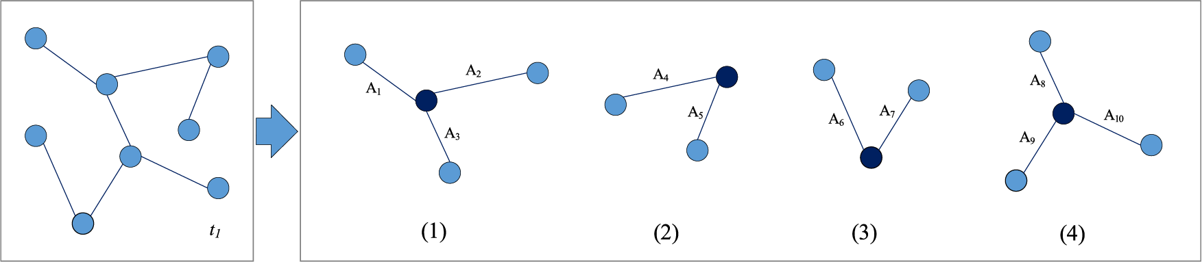
Figure 3: Handle some complex topology structures at a time t1

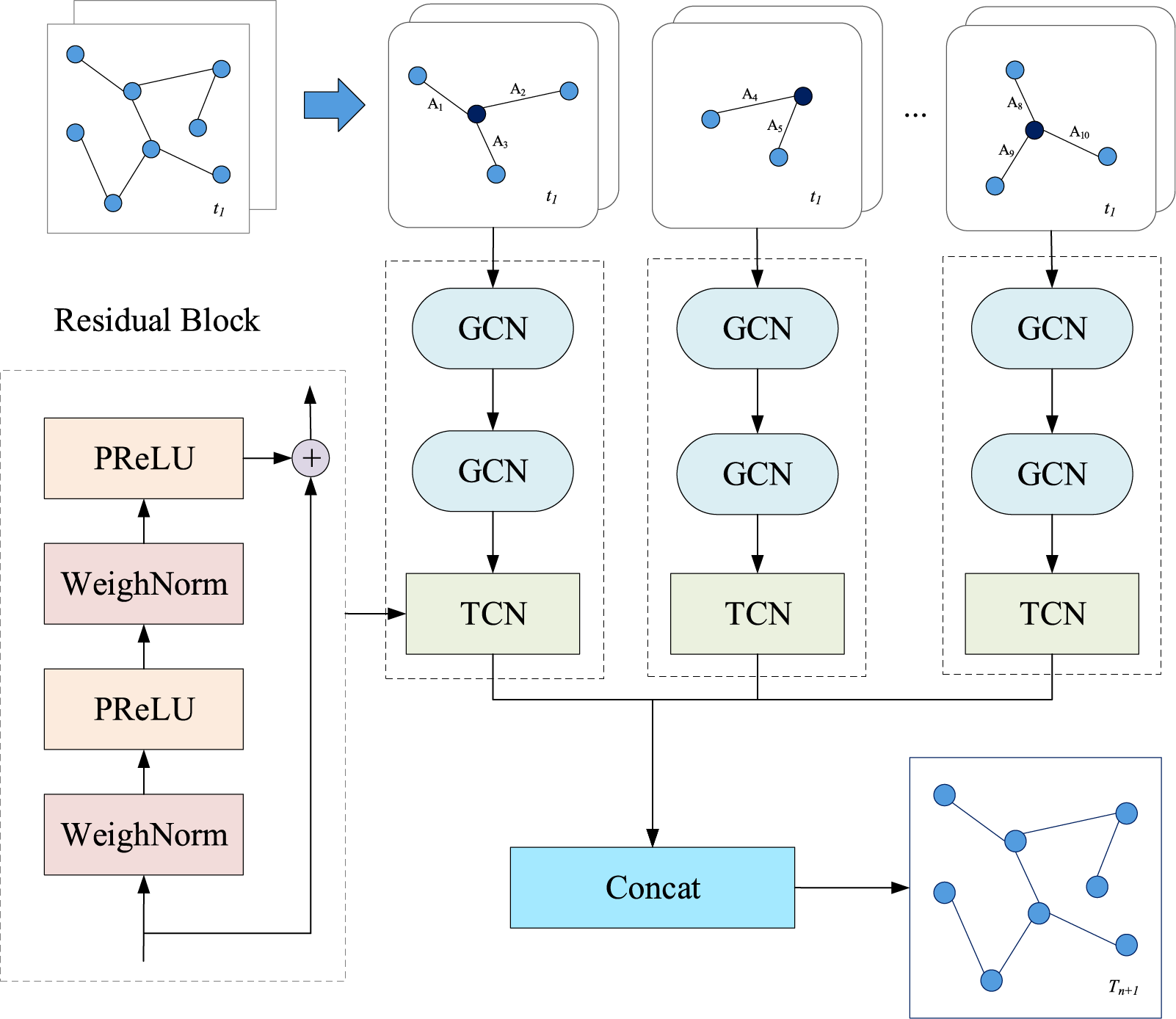
Figure 4: The structure of FAGTN

4  Construct a Spatiotemporal Feature Analysis Model

STD’s accuracy detection is influenced by time series and entity space features. This article constructs the spatiotemporal feature analysis model and gives the model design idea and model framework.

4.1 Model Design Ideas

GCN’s core is to define convolution operations on graphs possessing complex topology structures to achieve spatial feature extraction. TCN’s core lies in performing convolutional operations on temporal data to learn temporal features. Based on this, this article fused GCN and TCN (named FAGTN) and made improvements, which are described below.

I. For enhancing the saliency of spatial feature extraction, this article proposes an adaptive weight coefficient calculation method.

II. This article chooses the PReLU activation function to improve the residual module for temporal feature extraction.

Unlike conventional image convolution operations, graphs with complex topology structures cannot be convolved in the spatial domain by conventional methods. Therefore, the concept of Fourier transform is introduced to transform the graph from the spatial domain view to the frequency domain view for processing. The scaling operation is performed on each dimension, and the adjacent nodes are aggregated to complete the convolution operation, and finally return to the Spatial domain. The transformation process is shown in formula (10).

Lx=UλUTx(10)

L(L=D−A) is the Laplacian matrix of the graph, and D is the degree matrix of the graph, which indicates the nodes’ connectivity in the graph. A indicates the graph’s adjacency matrix, which x is a n dimension column vector that represents the node’s characteristics. Both U and UT are orthogonal matrices. To solve the problem of gradient disappearance or gradient explosion caused by the increased number of calculations, the Chebyshev polynomial is used as the restriction function of matrix eigenvalue A. After the regularization and renormalization tricks, the formula for calculating one layer GCN in FAGTN is obtained as shown below.

X(n+1)=σ(AX(n)W)(11)

X represents the characteristic matrix, σ represents the non-linear activation function. Transform the adjacency matrix according to A=D−12A~D−12 and A~=I+A, and W represents the trainable weight matrix. For enhancing the saliency of spatial feature extraction, this article proposes an adaptive weight coefficient calculation method to preprocess complex topology structures and generate a weight matrices corresponding to each detection space. Meanwhile, this article uses two graph convolution layers to implement spatial feature extraction to avoid the Over-Smoothing phenomenon.

This article introduces and improves TCN, which solves the problem of learning temporal features. A one-dimensional fully convolutional network structure (FCN) is adopted to ensure the same length between layers by zero padding. Dilated causal convolutions are added to achieve exponential expansion of the receptive field. At the same time, it also ensures that the output at a certain time is only convolved with elements at that time and earlier. When training a deeper network structure, the residual connection structure is used to transfer information across layers. This article selects the PReLU activation function to improve the residual module and enhance the ability that the model to learn effective temporal features by training the learnable parameters θ. The formula for calculating one layer TCN in FAGTN is obtained as shown below.

H(s)=∑f(⋅)XF(x)(12)

f(⋅) represents the convolution kernel, X represents the time series data, F(x)=Wσ(⋅)+α means residual function, W means weight function, σ(⋅) means the activation function.

4.2 Framework and Algorithm Implementation of FAGTN

The structure of FAGTN (spatiotemporal Feature Analysis Model Fused by GCN and TCN) is shown in Fig. 4. FAGTN consists of three modules: complex topology structure processing module, spatiotemporal feature extraction module, and spatiotemporal fusion convolution module. Firstly, this article converts the complex topology structure into a graph model for processing, and outputs a detection space with a weight matrix; secondly, this article achieves spatial feature extraction by stacking two layers of GCN, and using one layer of TCN to complete temporal feature extraction; finally, this article obtain the network output by fusing spatiotemporal features through convolution operation.

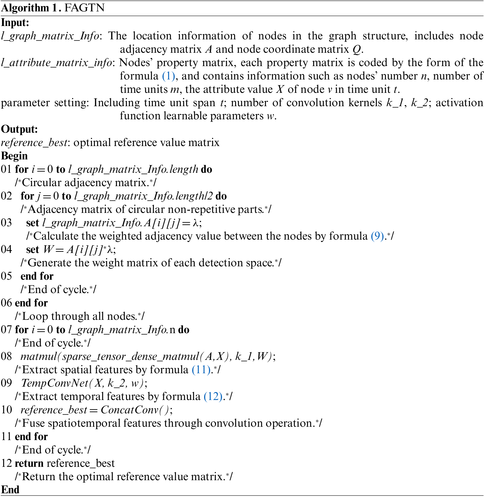
The pseudo-code form of FAGTN is shown in Algorithm 1, wherein, “/**/” indicates the annotation.

4.3 Evaluation Function of FAGTN

This article uses three evaluation metrics to evaluate the accuracy of FAGTN. They are the root mean square error (RMSE) [33], the mean absolute error (MAE) [34], and the mean absolute percentage error (MAPE) [35]. The specific calculation formula is as follows.

PRMSE=1γ∑(X^vit+1−Xvit+1)2(13)

PMAE=1γ∑i=1γ⁡|X^vit+1−Xvit+1|(14)

PMAPE=1γ∑i=1γ⁡|X^vit+1−Xvit+1|Xvit+1(15)

Xvit+1 represents the actual value of the node vi at the next time point (t+1), X^vit+1 means the reference value of the node vi at the next time point (t+1), and γ indicates the number of nodes. Both RMSE and MAE can reflect the error between the actual value and reference value, and the smaller value of both, the higher model’s accuracy will be. MAPE can reflect the ratio between error and actual value.

5  Example Verification

In this part, this article verifies the effectiveness of the spatiotemporal heterogeneity data accuracy detection method proposed in this article by comparing the performance indicators of a similar model. A brief description of the experimental design is shown below.

I. Explain the experimental preparation work. Introduce the experimental environment, experimental data, and comparison model.

II. Analyze the performance indicators’ changes of FAGTN and comparison model in various conditions, to demonstrate that FAGTN has obvious advantages in detection speed, model accuracy, and stability.

III. Compare the performance indicators’ changes of FAGTN and comparison model before and after handling complex topology structure, and discuss the influence of handling complex topology structure on the detection speed and model accuracy.

5.1 Experiment Preparation

I. Experimental environment. This article simulated the subsystem of the data quality inspection system of an onshore oilfield in the laboratory. The simulation environment structure is shown in Fig. 5. In the real environment, the control center is responsible for the intelligent scheduling of resources, the convergence platform is responsible for data detection tasks, the data center is responsible for providing data support, and the detection model is responsible for data accuracy detection.

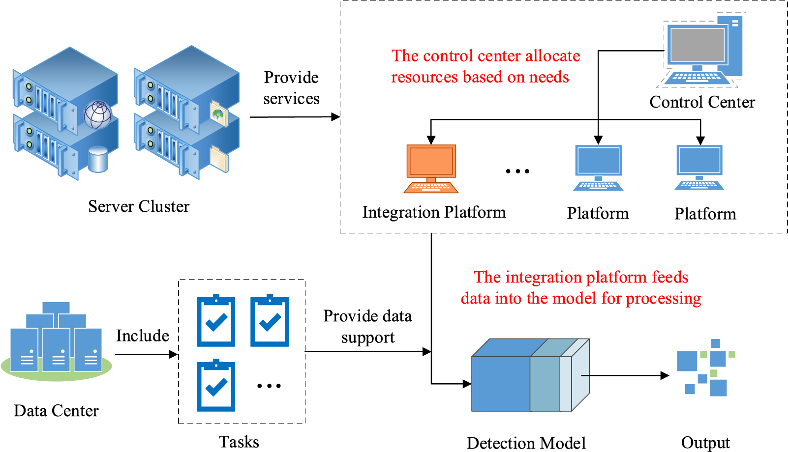
Figure 5: Experimental environment structure

II. Data description. This article took the accurate detection of oilfield data as the engineering background, selected an oilfield as the target area for the study, and chose real data sets from the oilfield to train and validate the model. The dataset contains key attributes of the field development dynamic data, such as well location information, well-to-well connectivity, and various parameters of the well at different periods. The target detection area contains multiple well groups, and each well group has no less than 130 wells. The well distribution and some wells’ connectivity in the target area are shown in Fig. 6.

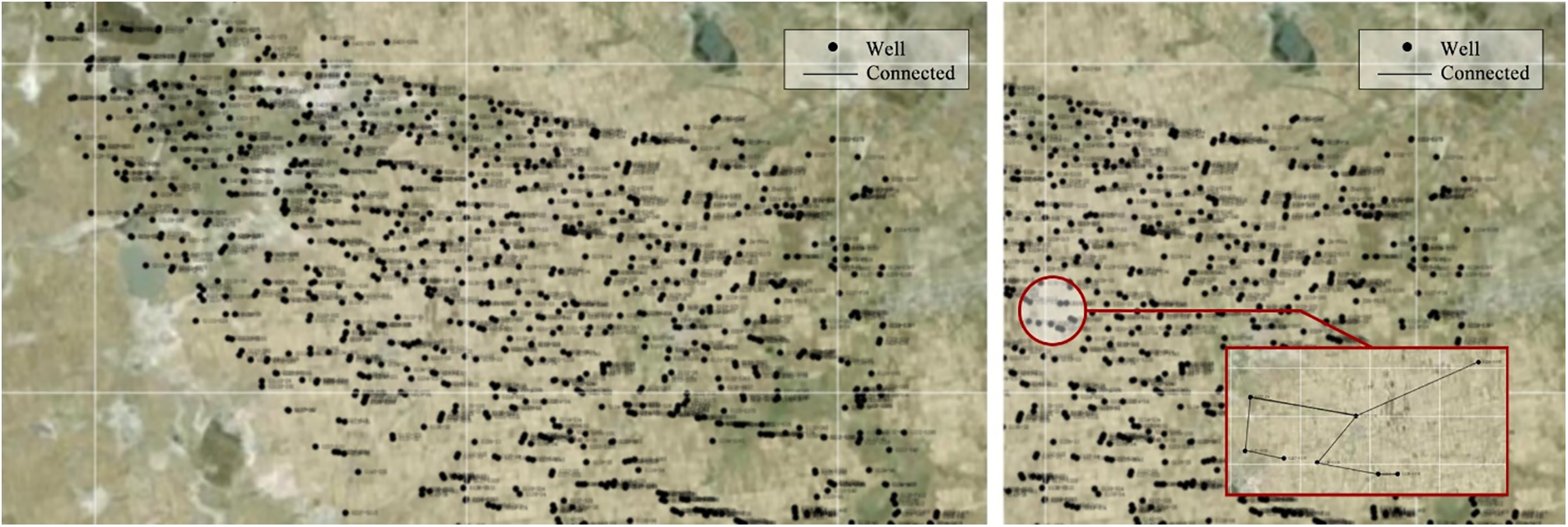
Figure 6: The well distribution and some wells’ connectivity in the target area

The oilfield data is summarized once a month. This article selected the data between 2008 and 2018, chose the first ten years as the training set, and the rest were used as the validation set and test set respectively. This article represented multiple attribute parameters of the data as different detection tasks, and wrote each data item as Data=⟨WellId:Time,Coordinate,Attributes[1],Attributes[2], Attributes[3],…⟩ .

III. Comparing model. The experiments involve the performance experiment of FAGTN, and the experiment of handling complex topology structures. This article selected ARIMA [36], T-GCN [32], and STGCN [37] as comparing models. These models are all used to solve the correlation analysis problem of spatiotemporal data.

5.2 Performance Test of FAGTN

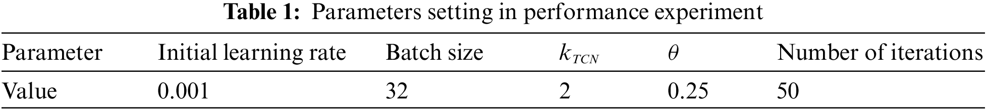
This article compared performance indicators of FAGTN, ARIMA, T-GCN, and STGCN in different levels of connectivity and different time periods. The performance indicators include the average detection time and the model accuracy. The aim is to verify that FAGTN has obvious advantages in terms of detection speed, detection accuracy, and stability. Table 1 shows the basic parameter settings of the model. kTCN represents the initial expansion factor in the temporal convolution module, θ represents the activation function parameter.

5.2.1 Performance Experiments with Different Degrees of Connectivity

This article tested the average detection time and the model accuracy obtained by the four models in different degrees of connectivity. This aims to observe the influence of the complexity of the connectivity between nodes on the detection speed and accuracy of the models.

In the performance experiment with different degrees of connectivity, this article divided the training set into two parts and defined the node set that satisfies |D|≥5 as the complex connected area, and the one that satisfies 0≤|D|≤4 as the simply connected area. This article selected an attribute of the data from January 2008 to December 2017 to participate in the experiment. The experimental results are shown in Table 2.

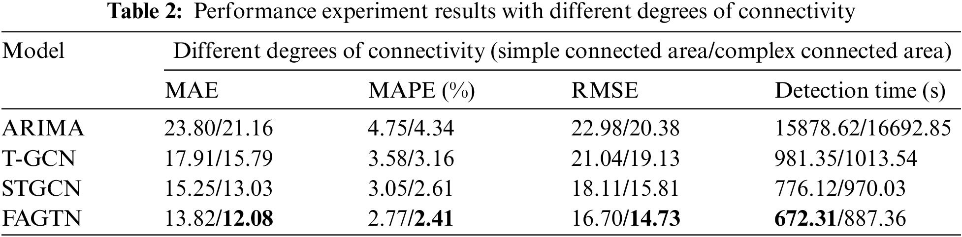
By analyzing the experimental results, this article obtained the following conclusions.

(1) The traditional time series model (ARIMA) performed poorly in the experiment. When dealing with STD, this model only considered the temporal characteristics of the data and ignored the spatial characteristics of the data, which is a poor fit for data with prominent spatiotemporal heterogeneity, so the accuracy of the model is lower.

(2) As shown in Table 2, T-GCN, STGCN, and FAGTN can better capture the spatiotemporal dependence of data. Comparing FAGTN and STGCN with good performance, this article found that the MAE, RMSE, and detection time of FAGTN are lower than STGCN, indicating that FAGTN has an execution efficiency superior to STGCN.

(3) When dealing with different degrees of connectivity, the four models all showed better performance in complex connected areas. It indicated that complex connected areas can adapt to deeper spatial feature mining.

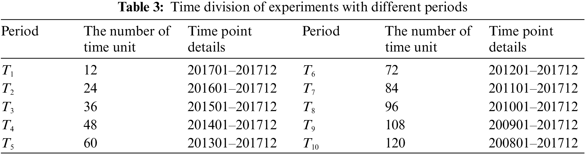
5.2.2 Performance Experiments with Different Periods

This article tested the model accuracy obtained by the four models in different periods. This aims to observe the influence of the historical time series length on the detection accuracy of the models.

In the performance experiment with different periods, this article selected all nodes to participate in the experiment. To highlight the influence of the length of the period on the model performance, this article divided the training set into 10-time units according to the year, and each time unit contained 12-time points corresponding to the 12 months of each year. This article designed a self-increasing time series Ti(1≤i≤10) and the increment is one time. The specific design is shown in Table 3.

Comparing the experimental performance of the four models, the experimental results are shown in Fig. 7.

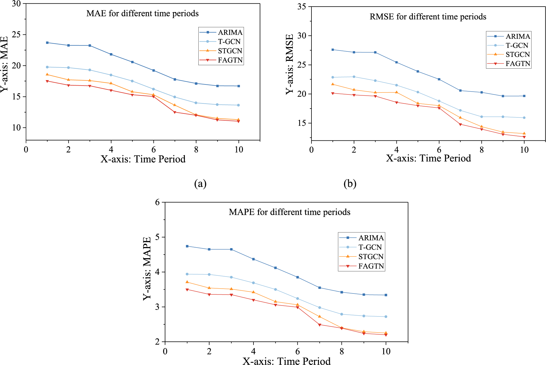
Figure 7: Different periods’ experiment results

By analyzing the experimental results, this article obtained the following conclusions.

(1) As shown in Figs. 7a–7c, with the increase of period, the accuracies of the four models all show an increasing trend. Among them, the effects of STGCN and FAGTN are significantly better than T-GCN and ARIMA models.

(2) Compared with the STGCN which has better performance, FAGTN’s performance always has obvious advantages in different periods. This article found that when the historical time series increases, the accuracy of FAGTN is always the highest, indicating that FAGTN maintains its advantages in the processing of long historical time series.

5.2.3 Stability Experiments of the Model

This article selected the STGCN which has better performance as the comparison model, and tested the models’ accuracy in different detection tasks and the different numbers of experiments. This aims to analyze the models’ stability. This article took the types of detection tasks and the number of experiments as variables and used the control variable method to test the changes in the accuracy of the model.

This article performed 5 groups of experiments for different detection tasks, selected different data attributes as detection tasks, and repeated each group of experiments 10 times. The experimental result is the average of all experimental results. Fig. 8a shows the influence of different detection tasks on the stability of the two models.

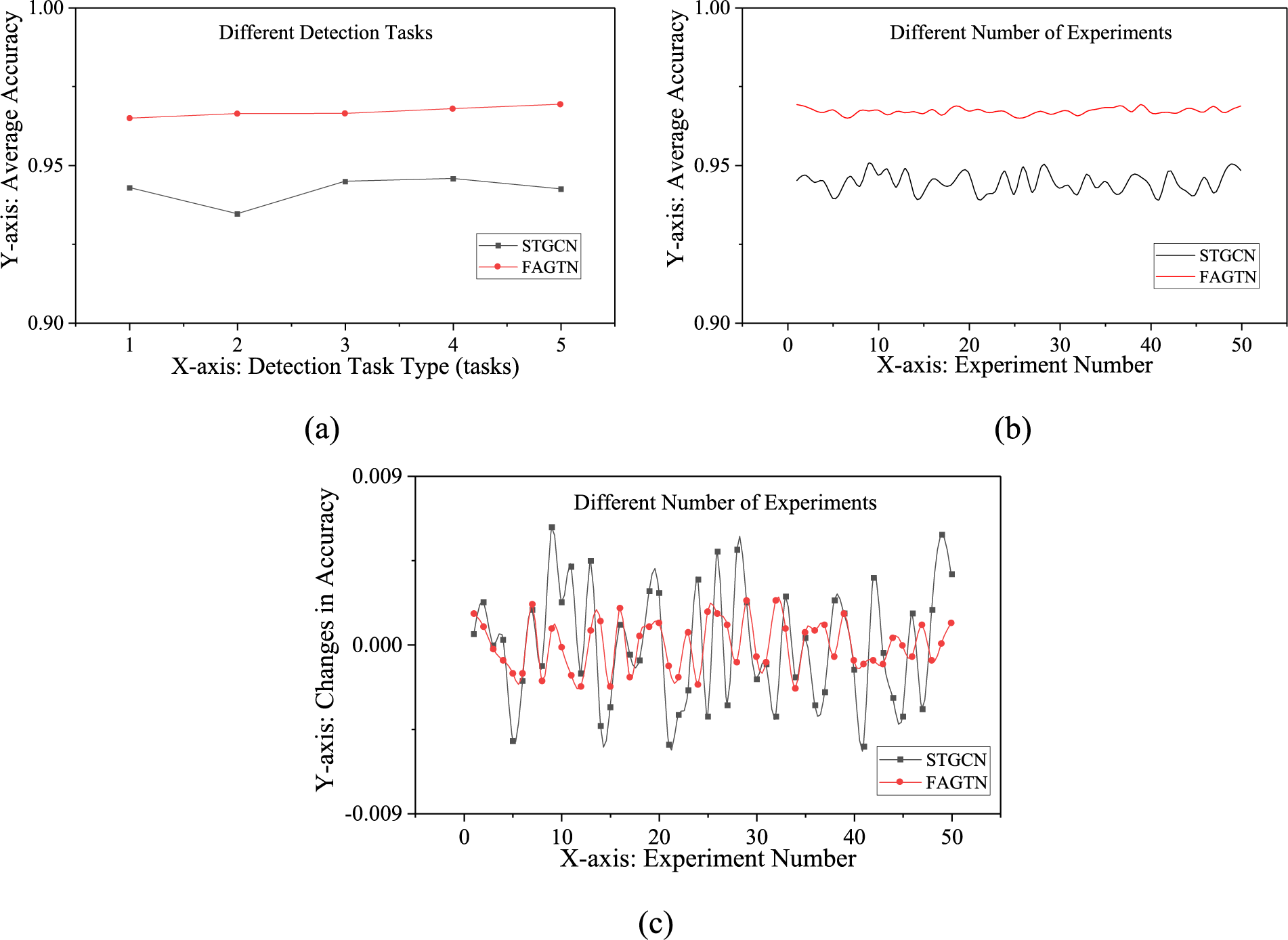
Figure 8: Experimental results of models’ stability

This article performed 50 groups of experiments for the different numbers of experiments added an experiment as a new group each time (the first group had one experiment), and took the average of the experimental results of each group. Figs. 8b–8c show the influence of the different number of experiments on the stability of the two models.

As a supplementary instruction, Table 4 shows the values of various indicators of the two models in the experiment.

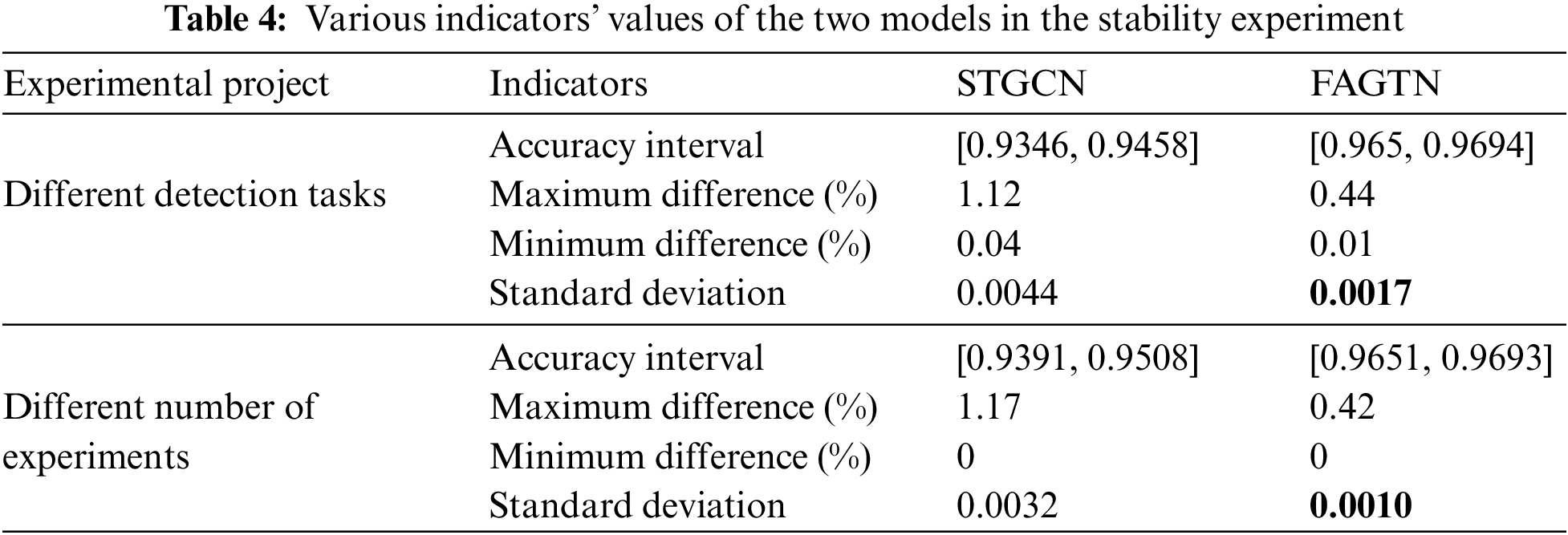
By analyzing the experimental results of the model’s stability, this article obtained the following conclusions.

(1) As shown in Fig. 9a, when the detection task changed, the two models’ accuracy both fluctuated within a certain range, and the standard deviation of the FAGTN was smaller than that of the STGCN. It indicated that FAGTN has stability superior to STGCN.

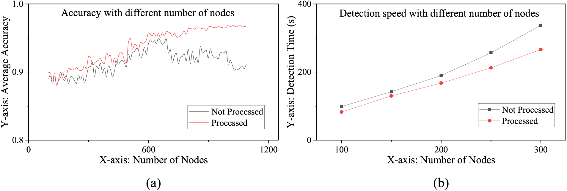
Figure 9: Influence of handling complex topology structure on the model

(2) As shown in Figs. 9a–9b, with the increase in the number of experiments, FAGTN’s accuracy fluctuation was significantly smaller than STGCNs’. The standard deviations for FAGTN and STGCN were 0.0032 and 0.001, respectively. Therefore, it indicated that FAGTN has stability superior to the STGCN in the different number of experiments.

5.3 Influence of Handling Complex Topology Structure on the Detection Accuracy and Speed

This article compared and analyzed the following indicators before and after handling complex topology structures.

I. The accuracy of the model before and after handling complex topology structures.

II. The average detection time of the model before and after handling complex topology structures.

This article designed this experiment to analyze the effect before and after handling complex topology structures on detection accuracy and detection speed. This article selected the number of nodes as a variable (the nodes in the experiment can form multiple detection spaces) and compared the models with different numbers of nodes. This article performed 100 groups of experiments for accuracy added 10 nodes as a new group each time (the first group has 100 nodes), and took the average of the experimental results of each group. This article performed 5 groups of experiments for detection speed and added 50 nodes as a new group each time (the first group had 100 nodes). The experimental results are shown in Fig. 9.

By analyzing the experimental results, this article obtained the following conclusions.

(1) As shown in Fig. 9a, with the increase of the nodes’ number, the accuracy of the model which preprocessed complex topology structure showed an upward trend. When the node reached a certain number, the accuracy fluctuation tends to level off. The accuracy of the model whose complex topology structure has not been preprocessed is generally lower than the model that has been preprocessed. When the node reached a certain number, the accuracy of the model showed a downward trend. It showed that the continuous increase of the nodes’ number will lead to the increase of invalid connectivity. If the complex topology structure was not preprocessed, the model’s ability to extract spatial features would be reduced.

(2) As shown in Fig. 9b, when the number of nodes increased, the detection time of the model also increased. The detection time of the model which preprocessed complex topology structure is generally lower than the model that is not preprocessed. It indicated that preprocessing complex topology structure had a certain effect on improving the model detection speed.

6  Conclusion

This article proposed a spatiotemporal heterogeneity data accuracy detection method by fusing graph convolution networks and temporal convolution networks, which are divided into two main stages. In the first stage, the geo-weighting function is improved, which in turn leads to a simplification of the complex topology. In the second stage, the spatiotemporal feature analysis model (FAGTN) is designed based on GCN and TCN to improve the detection speed and accuracy. Summarized as follows.

I. The experimental results show that compared with similar models, FAGTN has obvious advantages in detection speed, detection accuracy, and stability.

II. The degree of connectivity between nodes and the historical time series length will affect the model’s detection speed and detection accuracy. When the two factors changed, compared with similar models, FAGTN had obvious advantages.

III. Preprocessing the complex topology structure can optimize the detection space and improve the detection accuracy of the model.

The problem of STD accuracy detection cannot be ignored. When applying the method proposed in this article to a real scenario, some more specific problems need to be solved. For example, how to add the influence of the nodes’ attribute value, and how to quickly model the node. These problems need to be further resolved in the future.

Funding Statement: This work was supported by the National Natural Science Foundation of China under Grants 42172161, by the Heilongjiang Provincial Natural Science Foundation of China under Grant LH2020F003, by the Heilongjiang Provincial Department of Education Project of China under Grants UNPYSCT-2020144, by the Innovation Guidance Fund of Heilongjiang Province of China under Grants 15071202202, and by the Science and Technology Bureau Project of Qinhuangdao Province of China under Grants 202101A226. The authors would like to express their gratitude to the anonymous reviewers, whose helpful comments and suggestions improved the quality of this article.

Conflicts of Interest: The authors declare that they have no conflicts of interest to report regarding the present study.

References

1. J. X. Zhang, Y. C. Feng and Z. Y. Zhu, “Spatio-temporal heterogeneity of carbon emissions and its key influencing factors in the Yellow river economic belt of China from 2006 to 2019,” International Journal of Environmental Research and Public Health, vol. 19, no. 7, pp. 4185, 2022. [Google Scholar] [PubMed]

2. K. Xiong, Z. Yang and B. J. He, “Spatiotemporal heterogeneity of street thermal environments and development of an optimised method to improve field measurement accuracy,” Urban Climate, vol. 42, pp. 101121, 2022. [Google Scholar]

3. G. Yu, Y. Wang, M. Hu, L. Shi, Z. Mao et al., “RIOMS: An intelligent system for operation and maintenance of urban roads using spatiotemporal data in smart cities,” Future Generation Computer Systems, vol. 115, pp. 583–609, 2021. [Google Scholar]

4. S. M. H. Hashemi, K. Monfaredi and B. Sedaee, “An inclusive consistency check procedure for quality control methods of the black oil laboratory data,” Journal of Petroleum Exploration and Production Technology, vol. 10, no. 5, pp. 2153–2173, 2020. [Google Scholar]

5. L. Tišljarić, E. Majstorović, T. Erdelić and T. Carić, “Measure for traffic anomaly detection on the urban roads using speed transition matrices,” in 2020 43rd Int. Convention on Information, Communication and Electronic Technology (MIPRO), Opatija, Croatia, IEEE, pp. 252–259, 2020. [Google Scholar]

6. L. Ben Amor, I. Lahyani and M. Jmaiel, “AUDIT: Anomalous data detection and isolation approach for mobile healThcare systems,” Expert Systems, vol. 37, no. 1, pp. e12390, 2020. [Google Scholar]

7. L. Maddalena, M. Giordano, M. Manzo and M. R. Guarracino, “Whole-graph embedding and adversarial attacks for life sciences,” in Trends in Biomathematics: Stability and Oscillations in Environmental, Social, and Biological Models: Selected Works from the BIOMAT Consortium Lectures, Rio de Janeiro, Brazil, pp. 1–21, 2021. [Google Scholar]

8. G. Mylavarapu, J. P. Thomas and K. A. Viswanathan, “An automated big data accuracy assessment tool,” in 2019 IEEE 4th Int. Conf. on Big Data Analytics (ICBDA), Suzhou, China, IEEE, pp. 193–197, 2019. [Google Scholar]

9. S. Juddoo and C. George, “A qualitative assessment of machine learning support for detecting data completeness and accuracy issues to improve data analytics in big data for the healthcare industry,” in 2020 3rd Int. Conf. on Emerging Trends in Electrical, Electronic and Communications Engineering (ELECOM), Balaclava, Mauritius, IEEE, pp. 58–66, 2020. [Google Scholar]

10. A. C. Rai, P. Kumar, F. Pilla, A. N. Skouloudis, S. D. Sabatino et al., “End-user perspective of low-cost sensors for outdoor air pollution monitoring,” Science of the Total Environment, vol. 607, pp. 691–705, 2017. [Google Scholar] [PubMed]

11. W. Zhao, X. Jiang and J. Wang. “Cloud data center intrusion detection model based on active rules,” in 2020 IEEE Conf. on Telecommunications, Optics and Computer Science (TOCS), Shenyang, China, IEEE, pp. 49–54, 2020. [Google Scholar]

12. B. Cui, S. He and H. Jin, “Multi-layer anomaly detection for internet traffic based on data mining,” in 2015 9th Int. Conf. on Innovative Mobile and Internet Services in Ubiquitous Computing, Santa Catarina, Brazil, IEEE, pp. 277–282, 2015. [Google Scholar]

13. S. Kang, S. Peng and S. S. Qu, “Spatial relationships-based data inconsistency detection for raster land cover,” Journal of Spatial Science, vol. 68, pp. 1–20, 2021. [Google Scholar]

14. F. González, D. Dasgupta and J. Gómez, “The effect of binary matching rules in negative selection,” in Genetic and Evolutionary Computation Conf., Springer, Berlin, Heidelberg, pp. 195–206, 2003. [Google Scholar]

15. T. N. Kipf and M. Welling, “Semi-Supervised Classification with Graph Convolutional Networks,” CoRR, vol.abs/1609.02907, 2016. [Google Scholar]

16. F. Monti, K. Otness and M. M. Bronstein, “Motifnet: A motif-based graph convolutional network for directed graphs,” in 2018 IEEE Data Science Workshop (DSW), Lausanne, L, Switzerland, pp. 225–228, 2018. [Google Scholar]

17. H. Y. Cui, G. K. Wang, Y. X. Li and R. E. Welsh, “Self-training method based on GCN for semi-supervised short text classification,” Information Sciences, vol. 611, pp. 18–29, 2022. [Google Scholar]

18. S. Li, J. Yi, Y. A. Farha and J. Gall, “Pose refinement graph convolutional network for skeleton-based action recognition,” IEEE Robotics and Automation Letters, vol. 6, no. 2, pp. 1028–1035, 2021. [Google Scholar]

19. X. Wang, X. Rong, Y. Cheng and Z. S. Cheng, “Multi-label image recognition based on adaptive multi-scale graph convolutional network,” Control and Decision, vol. 37, no. 7, pp. 1737–1744, 2022. [Google Scholar]

20. Y. Djenouri, A. Belhadi, E. H. Houssein, G. Srivastava and C. W. Lin, “Intelligent graph convolutional neural network for road crack detection,” IEEE Transactions on Intelligent Transportation Systems, pp. 1–8, 2022. https://doi.org/10.1109/TITS.2022.3215538 [Google Scholar] [CrossRef]

21. X. Chen and V. Dinavahi, “Group behavior pattern recognition algorithm based on spatiotemporal graph convolutional networks,” Scientific Programming, vol. 2021, pp. 1–8, 2021. [Google Scholar]

22. S. Bai, J. Z. Kolter and V. Koltun, “An empirical evaluation of generic convolutional and recurrent networks for sequence modeling,” arXiv preprint arXiv:1803.01271, 2018. [Google Scholar]

23. C. Lea, M. D. Flynn, R. Vidal, A. Reiter and G. D. Hager, “Temporal convolutional networks for action segmentation and detection,” in Proc. of the IEEE Conf. on Computer Vision and Pattern Recognition, Honolulu, HI, USA, pp. 156–165, 2017. [Google Scholar]

24. S. Q. Cao, L. B. Wu, J. Wu, D. Wu and Q. Li, “A spatio-temporal sequence-to-sequence network for traffic flow prediction,” Information Sciences, vol. 610, pp. 185–203, 2022. [Google Scholar]

25. Z. Wang, J. Tian, H. Fang, L. Chen and J. Qin, “LightLog: A lightweight temporal convolutional network for log anomaly detection on the edge,” Computer Networks, vol. 203, pp. 108616, 2022. [Google Scholar]

26. Q. Zhao, Y. Zhang and X. Feng. “Predicting information diffusion via deep temporal convolutional networks,” Information Systems, vol. 108, pp. 102045, 2022. [Google Scholar]

27. T. Ni, X. Ding, Y. Wang, J. Shen and L. F. Jiang, “Spectrum sensing via temporal convolutional network,” China Communications, vol. 18, no. 9, pp. 37–47, 2021. [Google Scholar]

28. Z. Zheng, Z. Zhang, L. Wang and X. Luo, “Denoising temporal convolutional recurrent autoencoders for time series classification,” Information Sciences, vol. 588, no. 2022, pp. 159–173, 2022. [Google Scholar]

29. S. Dey, A. K. Dey and R. K. Mall, “Modeling long-term groundwater levels by exploring deep bidirectional long short-term memory using hydro-climatic data,” Water Resources Management, vol. 35, no. 10, pp. 3395–3410, 2021. [Google Scholar]

30. Z. Chen, B. Zhao, Y. H. Wang, Z. T. Duan and X. Zhao, “Multitask learning and GCN-based taxi demand prediction for a traffic road network,” Sensors, vol. 20, no. 13, pp. 3776, 2020. [Google Scholar] [PubMed]

31. Z. Jiang and X. Liu, “Adaptive KNN and graph-based auto-weighted multi-view consensus spectral learning,” Information Sciences, vol. 609, pp. 1132–1146, 2022. [Google Scholar]

32. L. Zhao, Y. Song, C. Zhang, Y. Liu, P. Wang et al., “T-Gcn: A temporal graph convolutional network for traffic prediction,” IEEE Transactions on Intelligent Transportation Systems, vol. 21, no. 9, pp. 3848–3858, 2019. [Google Scholar]

33. A. L. Schubert, D. Hagemann, A. Voss and K. Bergmann, “Evaluating the model fit of diffusion models with the root mean square error of approximation,” Journal of Mathematical Psychology, vol. 77, pp. 29–45, 2017. [Google Scholar]

34. N. G. Reich, J. Lessler, K. Sakrejda, S. A. Lauer, S. Iamsirithaworn et al., “Case study in evaluating time series prediction models using the relative mean absolute error,” The American Statistician, vol. 70, no. 3, pp. 285–292, 2016. [Google Scholar] [PubMed]

35. D. A. Fadare, “The application of artificial neural networks to mapping of wind speed profile for energy application in Nigeria,” Applied Energy, vol. 87, no. 3, pp. 934–942, 2010. [Google Scholar]

36. B. M. Williams and L. A. Hoel, “Modeling and forecasting vehicular traffic flow as a seasonal ARIMA process: Theoretical basis and empirical results,” Journal of Transportation Engineering, vol. 129, no. 6, pp. 664–672, 2003. [Google Scholar]

37. B. Yu, H. Yin and Z. Zhu, “Spatio-temporal graph convolutional networks: A deep learning framework for traffic forecasting,” arXiv preprint arXiv:1709.04875, 2017. [Google Scholar]