Ligand Based Virtual Screening of Molecular Compounds in Drug Discovery Using GCAN Fingerprint and Ensemble Machine Learning Algorithm

1  Introduction

Drug Discovery is one of the most difficult tasks in biomedicine today. High-Throughput Screening (HTS) analyses are performed to find compounds with optimistic bioactivity within the produced compound library. Although HTS studies are extremely effective, they are also costly in terms of time and money due to a large number of manufactured chemicals, protein supplies, and laboratory bioactivity testing procedures [1]. The Discovery of a drug is a very tedious and time-consuming process. The process involves experimenting with every sample compound available in the compound database to form the potential drugs. Currently, drug designing has evolved from Drug Discovery into Computer-Aided Drug Discovery (CADD). This change was brought about by several factors. One of these reasons is the low success rate of separating compounds into drugs and non-drugs. This has sparked renewed interest in better understanding what makes a compound drug like, as well as new models and methods for compound classification. There are two main methods for screening the drug similarity of a chemical compound. The methods are Ligand-Based Virtual Screening and Structure-Based Virtual Screening. When screening compounds, structure-based virtual screening is used if the structure of the target protein is already known. Ligand-based screening is the process to screen if the target protein is unknown. Many studies are rapidly proceeding in these two categories to convey more effective methods for the prediction of drug-likeness. Ligand-based methods for drug similarity prediction are primarily based on molecular descriptors and the representation of descriptors in the form of molecular fingerprints. Various fingerprint encoding methods are available for drug similarity prediction. The molecular fingerprints of the compounds are analyzed for molecular similarity. Because of advances in computational science, the discovery and development of new drugs have been accelerated. Artificial Intelligence (AI) is being used by an increasing number of businesses and academic institutions. Machine Learning (ML) is a key component of AI that has been integrated into a variety of industries including data collection and analytics. For algorithmic techniques like Machine Learning (ML), a solid foundation of mathematics and computational theory is required. Deep Learning (DL) assisted self-driving cars, advanced voice recognition, and Support Vector Machine (SVM) based smarter search engines are all examples of ML models being applied in promising technologies [2–5]. Drug discovery, bioinformatics, and cheminformatics have already benefited from the use of these computer-aided computational approaches initially developed in the 1950s. There are two basic categories of LBVS approaches such as similarity search and compound categorization [6]. Similarity search utilizes molecular fingerprints such as those derived from molecular graphs (2D) or conformations (3D), 3D pharmacophore models [7], simplified molecular graph representations [8], or molecular shape queries [9]. When a compound is compared to a database compound, a similarity metric produces a ranking of compounds in decreasing order of molecular similarity to reference molecules [10]. Candidate compounds are chosen based on their position in this similarity list. Tanimoto coefficients are commonly used as a measure of similarity for fingerprint or feature set overlap. After fingerprint generation, classification methods are applied to discover unseen drugs. Aside from basic classification methods like clustering and partitioning, machine-learning approaches like support vector machines (SVM), decision trees, k-nearest neighbours and artificial neural networks (ANN) are becoming increasingly popular in the classification of large-scale datasets of LBVS All of these strategies aim to predict compound class labels (e.g., active or inactive) based on models developed from training sets, as well as provide a ranking of database compounds based on the likelihood of their molecular fingerprint In addition, compounds can be selected for the construction of target-focused compound libraries Sub-structural analysis (SSA), presented by Cramer et al., as a technique for the automated interpretation of biological screening data, was the first application of machine learning in drug discovery The growing availability of massive data collections of various kinds has sparked interest in the development of novel data mining methods in the field of machine learning. When it comes to drug development, machine learning methods have a wide range of potential applications, so it’s worth having a glimpse at specific approaches and emphasizing their benefits. Because machine learning approaches are difficult to describe, incorporating them may consider them even more difficult to recognize. Graph Neural Network is the most efficient way of generating fingerprints from drug compounds. Traditional Graph Neural Networks ignore different hop neighbors. Exclusively the largest sub-graph which is the final aggregation output is used to learn the node representation. When a model is generated using an average/sum pooling method or a maximum pooling method, it may contain an excessive amount of irrelevant data. To address the aforementioned issues, we proposed a graph neural network with an attention mechanism, with ensemble modeling used for classification. The following are the main contribution of this paper: As an alternative to k-hop convolution, we propose a graph convolution method with an attention mechanism that can utilize information from distinct hop neighbors. The attention polling layer is used instead of the average or max-pooling layer which extracts all the information without losing individual node information. Later, the ensemble Model is used for drug classification. We conduct experimental analysis and compare with the existing fingerprint methods and model classification is compared with other existing models.

The organization of this article is structured accordingly. The related work is discussed in Section 2. The proposed approach is described in Section 3. Section 4 includes an experimental result analysis of the proposed method and finally, Section 5 concludes the research work.

2  Related Study

Numerous ML algorithms are being developed and utilized in all stages of drug discovery and development including the development of new targets, improvement in clinical trials, stronger evidence for target disease associations, improved small molecule compound design optimization, increased understanding of disease mechanisms, increased understanding of the disease, non-disease phenotypes, and the development of new biomarkers for prognosis efficacy [11]. In general, drug classification is divided into two stages. Initially, molecules are represented by encoding their structural information, and then this structural information is subsequently used as input to machine learning models for classification. Drug discovery applications rely on accurately describing molecules by encoding their structural information, which is a difficult problem in cheminformatics and machine learning to solve. Although there are many different types and applications for Molecular representations, molecular fingerprints are the most extensively used and recognized representations [12]. Molecular fingerprints can be pre-defined structural components such as PubChem fingerprints, which comprise 881 bits that reflect common substructures. The most advanced fingerprints are ECFPs which are a variation of the Morgan method. Using fingerprints, it is possible to compare molecules based on their similarity, which can be utilized in fingerprint-based virtual screening to identify potential drug candidates. They are employed in the analysis of virtual chemical libraries to identify molecules that are similar in structure and presumably similar in bioactivity. The selection of a fingerprint is critical to the performance of a similarity search of this nature, as different fingerprints target different chemical domains and attributes than others. Machine Learning (ML) based algorithms can be used to find compounds of interest that are bioactive. Based on their fingerprints, machine learning models can anticipate the actions of molecules rather than searching for similar compounds [13]. These methods do not require a similarity search, but they still rely on pre-calculated fingerprints at their heart. Graph Neural Networks (GNNs), a novel family of machine learning algorithms, may be able to eliminate the need to calculate fingerprints. When trained, these networks learn how to encode molecules directly and can manage them. As a result, GNNs can tailor their molecule-transformation strategies to the specifics of the task at hand. While standard fingerprints are unable to learn and encode structural information essential for a particular job. The initial method named ECFP discusses the use of Graph Neural Networks in the context of molecular fingerprints. The GNN outperforms the ECFP in many ways. The concept of chemical fingerprints was further developed in later research with more complex models. A Graph Neural Network that has been trained on molecules has the same capabilities as any other neural network that has been trained on molecules. These fingerprints are produced solely by the activation of a specific hidden layer in the network. Until now, research has concentrated on the potential for GNNs to improve prediction [14]. One or two studies have looked at how well these networks perform in terms of producing high-quality fingerprints. The chemical space covered by their fingerprint is compared to that of the ECFP. The ECFP and GNN fingerprints are compared, as previously indicated. Using an auto-encoder neural fingerprint, a similarity search is performed in a work. Those fingerprints, on the other hand, are formed by unsupervised training. While unsupervised models are trained to reconstruct or translate chemical representations, supervised models are trained to perform a specific goal, such as predicting a molecule’s activity. This enables unsupervised models to be utilized across multiple domains, but they cannot encode domain or task-specific information that supervised models accomplish. Until now, the performance of fingerprints derived from supervised models in terms of similarity search has been ignored. ECFP is a widely used circular fingerprinting algorithm that encodes molecular structure by hashing fragments up to a certain radius. An ECFP fingerprint, on the other hand, is often difficult to decipher [15]. Combining multiple types of fingerprints with different machine learning methods is an ideal strategy that can improve the model’s diversity and consequently its prediction ability, according to current research As far as model creation is concerned, ensemble modeling can adequately combine the predictions of multiple models [16]. Since each base learner’s strengths and weaknesses are taken into account, ensemble learning tends to be more accurate than individual models recent work using ensemble learning for chemical toxicity prediction has shown promising results [17] were able to develop a predictive ensemble model with an accuracy of 89 percent [18]. With an accuracy of 86%, drug classification based on a set of nine molecular fingerprints has been proposed using ensemble modeling.

3  Proposed Method

The proposed ligand-based virtual screening drug discovery framework is shown in Fig. 1 [19]. It is divided into two major components: Molecular Fingerprint Generation and drug prediction using the Ensemble approach [20].

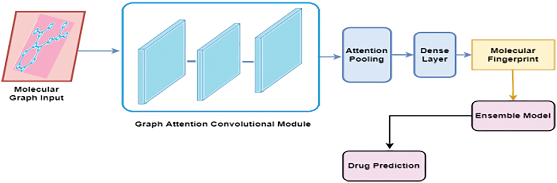
Figure 1: Proposed model

3.1 Molecular Fingerprint Generation

In our proposed method, fingerprints are generated using an improved graph convolutional neural network known as Graph Convolutional Attention Network (GCAN) [21]. The attention pooling layer is used instead of the mean/max-pooling layer as in the traditional graph convolutional neural network. The improved graph neural network consists of three major parts namely, the graph convolutional layer, attention convolutional layer, and attention pooling layer. The molecule can be considered as an undirected graph if the atoms in the compound are considered nodes and the bonds are considered edges of the network [22]. It is possible to use the graph convolutional neural network model to combine information from distant atoms along the bond direction [23]. All substructure identifiers are generated by adaptive learning in the differentiable network layers [24]. Using this method, it is possible to extract useful representations. Simplified Molecular Input Line Entry Specification (SMILES) strings are preferably converted to molecular graphs using RDKit, open-source cheminformatics software [25]. It is possible to encode molecules into ASCII strings using the SMILES specification, [26] which describes molecular 3D structures in ASCII. Each atom and the bonds that bind to it are then given a feature vector [27]. There are several aspects of the atoms and bonds in this vector, such as their element, their degree, and the number of hydrogen atoms attached to them [28]. The features of the bonds include their kind (single, double, triple, or ring), as well as their conjugation. It is possible to perform convolution operations at different levels when considering the different contributions made by neighboring atoms [29]. This is accomplished through the use of graph convolutional modules, which are comprised of graph convolutional layers, batch normalization layers, and graph pool layers [30].

3.2 Graph Convolutional Layer

Graph Convolutional Layer can be represented recursively followed by a convolutional structure with depth n as in Eq. (1).

Nn+1=ϕ(M^D−1^NnW)(1)

where Nn represents properties of nodes that contain the local structural information in the vector form. M^=M+I is the adjacency matrix with each node’s self-connection, D^ is the diagonal node degree of the adjacency matrix, M^D−1^ is the normalized graph structure in the convolutional layer and W is the weight parameter. The results of each step can only be used to construct the next convolution result during the recurrence of Eq. (1), except for the Nn parameter. There will be a significant loss of information during this process, and only the final convolution result from Nn, which represents the largest sub-graph and will be useful for subsequent tasks. This type of operation has the potential to result in a large loss of information. The convolutional layer would only capture the n-hop local structure. To address this problem, an attention convolution layer is implemented to focus on accumulating information from each convolution phase.

3.3 Attention Convolutional Layer

The core concept of the attention convolution layer in graph convolutional architecture is to improve the model’s ability to rely not only on the n-hop convolution output but also to capture valuable information from every hop in the process. Consequently, a hierarchical representation of the most valuable information from distinct hop convolution operations will be produced as a result of the convolution process. The hierarchical representation is defined by Eq. (2) as given below:

ρv=∑i=1nAiNvn(2)

Aggregation of each hop result is obtained by using the vanilla attention mechanism, where A is the attention weight, v  is the local structure in each hop and Nvn represents the node in the network. The information about the hierarchical structure is preserved inside the final node representation. Each attention convolutional layer’s input is the sum of the output of the layer before it and the original Y as illustrated in Fig. 2. This is known as the attention convolutional layer input. Finally, a dense layer is employed to analyze the combination of outputs from each convolution layer. These are denoted as the Attention Convolution Modules in Eqs. (3) and (4).

ρvm+1=∑i=1nAiNvnNv0=ρvm+Y(3)

ρv=Dense({ρv0, ρv1,…,ρvm},0)(4)

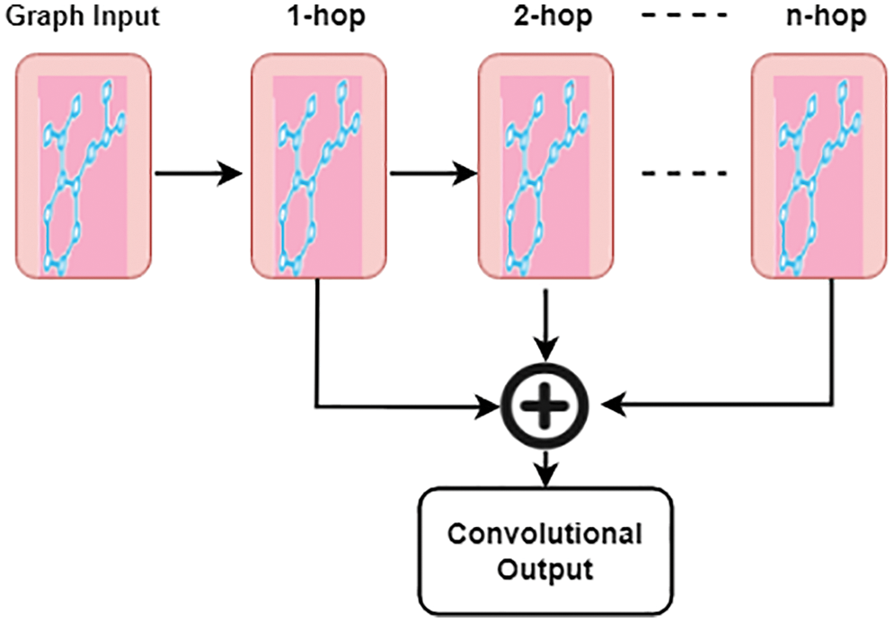
Figure 2: Attention convolutional layer

where Dense ( ) is the dense layer that sums up the output of all attention convolutional layers.

3.4 Attention Pooling Layer

Instead of relying on basic max/mean pooling after sorting, an attention pooling layer is proposed as a replacement for these methods. An arbitrary network is encoded into a fixed-size embedding matrix while maximizing the information contained inside each node’s depiction is the main goal of the attention pooling layer. The attention mechanism is utilized to produce the weights vector by considering the graph node representation learned from the convolution module as an input and outputting it as a weights vector A using the attention mechanism. When the hyperparameter r is selected for the number of subspaces, the graph representation from the node representation is learned to obtain the value higher than or equal to one. The attention weight is represented as a matrix  cxr rather than a vector in the pooling layer and c is the channel content feature in each node. It can be defined as in Eq. (5).

E=softmax(e1tanh⁡(e2DT))(5)

where e1  and e2 are the weight matrix with the cxc and cxr respectively. E  represents the weight of each node in different subspaces and D={ρv0, ρv1, …, ρvm}. Then, graph representation matrix H of a molecular fingerprint is get by weighted summation of  E,

 H=ED˙(6)

3.5 Ensemble Learning

This study employs six machine learning algorithms as a baseline model namely Support Vector Machine (SVM), Random Forest, Naïve Bayes, Decision tree, AdaBoost, and Gradient Boosting. The algorithms are explained in detail below:

•   Naïve Bayes (NB) Algorithm: Probability and likelihood are the underlying concepts of a Gaussian naive Bayes (NB) model. The algorithm is stable, quick, and straightforward. The foundation of NB is Bayes’ theorem, which is predicated on the strong assumption of conditional independence. Each feature in a class is presumed to be separate and distinct from the other features in that class. The model can be easily constructed and is beneficial for dealing with very large datasets. It can also outperform other classification methods. However, the Naïve Bayes algorithm performs better with categorical input variables than with numerical values and multiple-class prediction. It is possible that the assumption of independence on which the algorithm is built does not always work perfectly.

•   Decision Tree (DT) Algorithm: Both categorical and continuous variables benefit from the decision tree technique. Based on the input attributes, decision tree classifiers build a tree-like model (formed from the training dataset) to generate predictions about the test data. An attribute is associated with each of the nodes in the tree’s internal structure, and each leaf node is associated with a class label. While the training dataset is split into smaller subsets in a Decision Tree, a single feature is placed at the top of the tree. Every subset is subjected to the same two stages, which are then repeated indefinitely. It is a straightforward method that can handle a large set of data.

•   Random Forest (RF) Algorithm: A random forest classifies data is utilized for finding the mean probabilistic prediction of each tree. Over-fitting is a problem with the decision tree method that can be avoided by using decision trees, which are similar to traditional decision trees. However, it is more difficult to decipher than a decision tree. In order to create a forest of unique trees, each decision tree is constructed using randomness.

•   Boosting Algorithms: Boosting is a technique for creating strong learners from weak learners, which involves combining weak classifiers into a single strong classifier and then testing the result. An adaptive boosting classification algorithm, also known as AdaBoost or Adaptive Boosting (AB), is a machine learning classification algorithm based on the idea of iteratively causing weak learners to learn a larger portion of the examples in the training data that are difficult to classify by assigning more weight to test sets that are frequently misclassified. The weak learners are made up of decision trees that have just one split, which is referred to as decision stumps. In the gradient boosting method, several weaker models are combined to create a stronger model that is then tested. Gradient Boosting (GB) is a method of reducing the loss function until the minimum test loss is achieved and then repeating the process.

•   Support Vector Machine (SVM): Statistical learning theory is used to develop an effective machine learning approach called Support Vector Machine (SVM), which examines the data required for classification and regression analysis. By using numerous kernel functions, this approach translates the properties of the input data into a much higher-dimensional space and then generates a hyperplane or set of hyperplanes in a high-or infinite-dimensional space to distinguish between positive and negative values. In this work, the SVM models are constructed with the assistance of the radial basis kernel function.

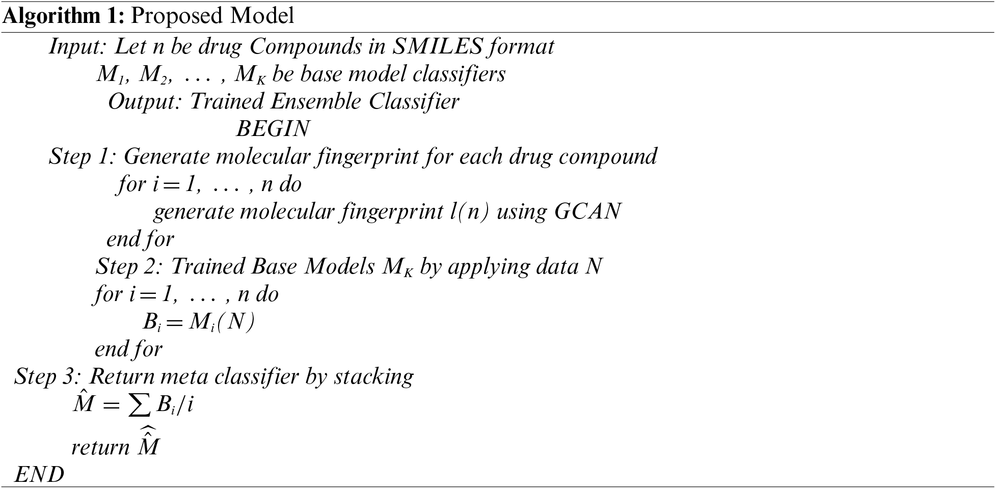
Generally expressing, the theory behind ensemble methods states that training data is evaluated in a variety of ways before an ensemble of first-stage classifiers is formed. A new ensemble classifier is built utilizing the stacked ensemble approach, in which a final-stage model learns how to combine the predictions from numerous first-stage models. A two-stage stacking strategy is employed. Initially, a dataset is used to train different models. The predictions of the first-stage models are then stored to create a new dataset. In the current dataset, each occurrence is linked to the actual estimate it is expected. The final prediction is made using the dataset and the meta-learning method. There are two types of models that make up a stacking model: Base Models (also called first-stage models) and meta-learner (final-stage classification). The training data is used to train various first-stage models. Subsequently, to integrate the base model predictions using previously unused data, the final-stage model is trained using the training dataset as well as the outputs of the first-stage models. Algorithm 1 describes the working process of the proposed model.

4  Experimental Analysis

4.1 Dataset

Bioactivity data from ChEMBL and PubChem were used to construct the dataset. More than 55,000 ligands have been tested on 160 human-protein kinases. All of the ligands were determined to be either active or inactive based on their ATP competitiveness. Numerous ligands in the dataset were tested on a few kinases, resulting in a lack of activity information for many kinases in the dataset. The final data set includes SMILES strings and kinase activation rates for each of the 160 compounds investigated. For the training, test, and external validation sets, a 5-fold cross-validation is employed with a random split of 80%, 10%, and 10%. An evaluation of the model’s performance, as well as its similarity, was carried out using an external set of data.

4.2 Evaluation Metrics

Base Models were tested using the following four indicators: Accuracy (ACC), Specificity (SPC), Sensitivity (SEN), and Area under Curve (AUC). ACC is a metric that measures the model’s capability to predict the expected data. SPC is used to assess predictive accuracy for negative data, while SEN is used to assess predictive accuracy for positive data. False positives (FP), false negatives (FN), and the number of true positives (TP) and false negatives (FN) can be used to calculate these three indicators (FN). The following are the results of the indicators’ calculation:

ACC=TP+TNTP+TN+FP+FN×100(7)

SPC=TNTN+FP×100(8)

SEN=TPTP+FN×100(9)

Receiving characteristic (ROC) curves are graphs that show the TP rate (SEN) vs. the FP rate (1-SPC) at various diagnostic cutoff points. The AUC was determined as a key measure of the model’s predictive value. In order to compare the efficiency of the generated molecular fingerprints, a similarity measure was utilized. The distance was calculated using continuous generalizations of the Tanimoto similarity metric. The distance calculation is given in Eq. (10).

 D(a,b)=1−∑min(ai, bi)∑max(ai, bi)(10)

The relationship between the distances and the correlation coefficient is 0.834.

There are two types of the experiment have been demonstrated to show the performance of the proposed fingerprint generation model. Initially, fingerprint similarity between Extended Connectivity Fingerprint (ECFP) and GCAN using their pairwise distance was examined as in Fig. 3. GCAN network compared with small and larger random weight initialization along with larger random weights. With larger random weights, the proposed model generates a fingerprint that is similar to the ECFP fingerprint.

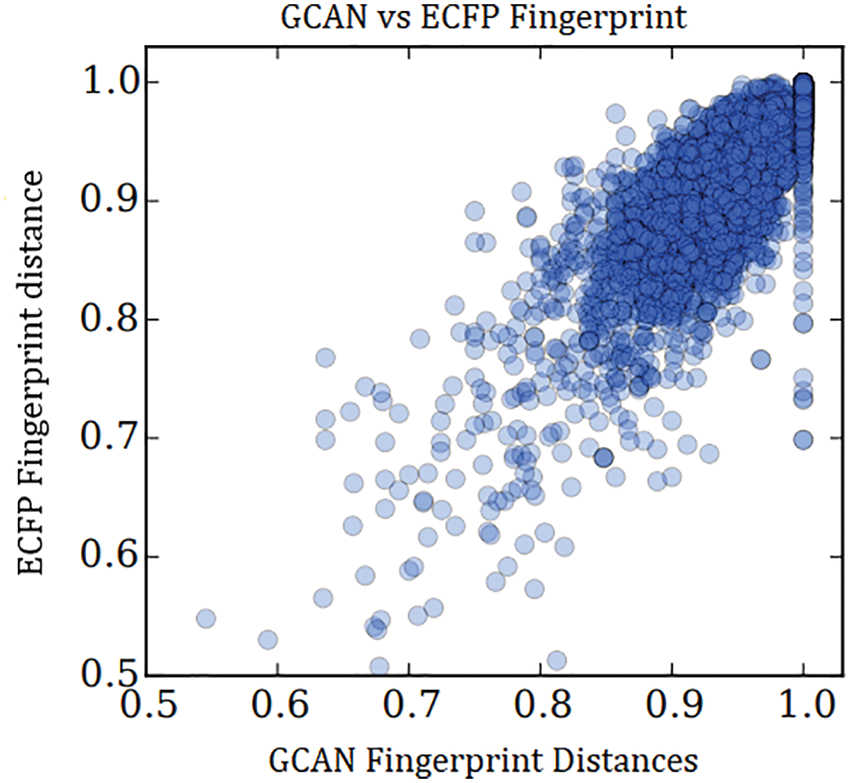
Figure 3: Similarity between ECFP and GCAN with large random weight

Secondly, neural fingerprints are compared with large and small random weights to ECFP fingerprints in terms of their predictive efficiency. Predictive analysis of Fingerprints with SVM gives a better result as shown in Fig. 4. which displays the average predictive performance. Both approaches produce similar results with larger random weights. Graph convolutional Attentional neural fingerprints with small random weights, on the other hand, have significantly better performance. In other words, the relatively smooth activation of neural fingerprints aids in generalization performance when weights are assigned at random. Before assembling, the fingerprint is used as input to the baseline classifier. Support Vector Machine (SVM), Random Forest, Naïve Bayes, Decision tree, AdaBoost, and Gradient Boosting are used as base classifiers. The performance of the baseline classifier with GCAN fingerprint is evaluated using 5-fold cross-validation and compared to the performance of the ECFP fingerprint. The learning rate for Graph Convolutional Neural Network (GCN) and Graph Convolutional Attention Network (GCAN) has been analyzed for both ChemBL and PubChem datasets. From Figs. 5 and 6, it is observed that the proposed method has performed better than traditional graph neural networks.

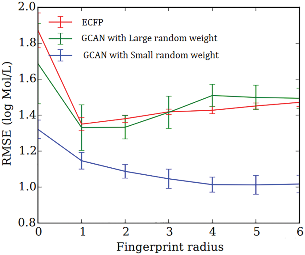
Figure 4: Average predictive performance of fingerprints

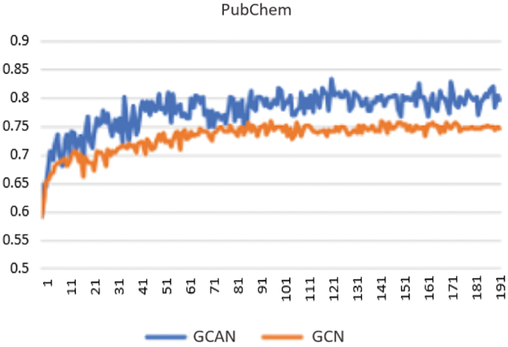
Figure 5: Learning curve using PubChem data

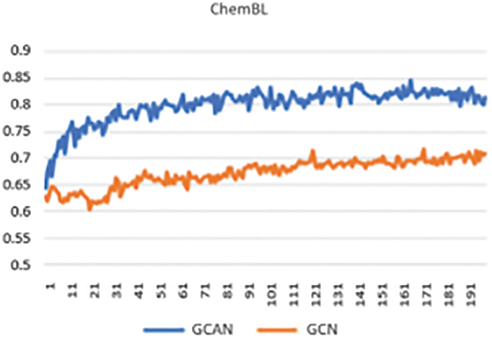
Figure 6: Learning curve using ChemBL data

Tables 1 and 2 show the performance of the baseline classifier using the ECFP fingerprint and the GCAN fingerprint, respectively. SVM outperforms other models in terms of ECFP and GCAN fingerprint accuracy. SVM achieves 89 percent accuracy with the ECFP finger but has lower specificity than other models. When compared to existing models, our suggested GCAN fingerprint has higher accuracy and specificity. Random forest, Nave Bayes, AdaBoost, and Gradient perform similarly, but our proposed technique outperforms ECFP fingerprint in terms of accuracy as shown in Figs. 7–9.

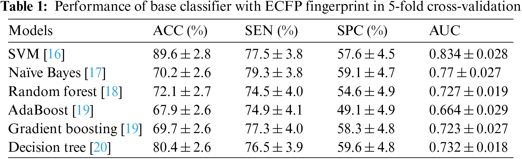
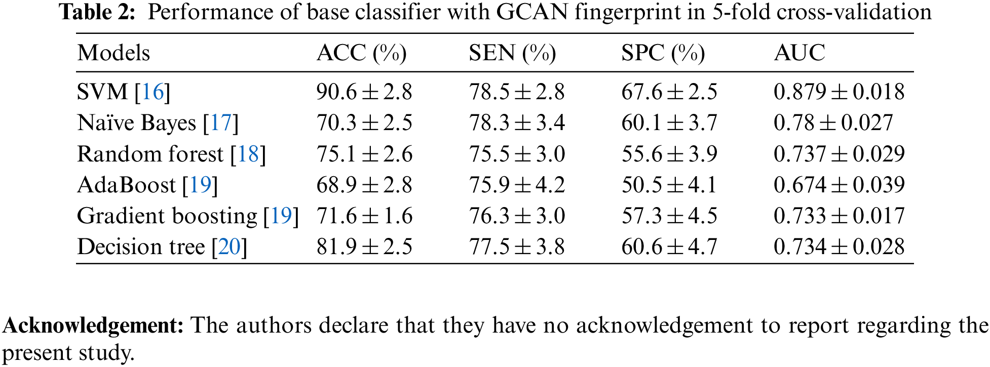
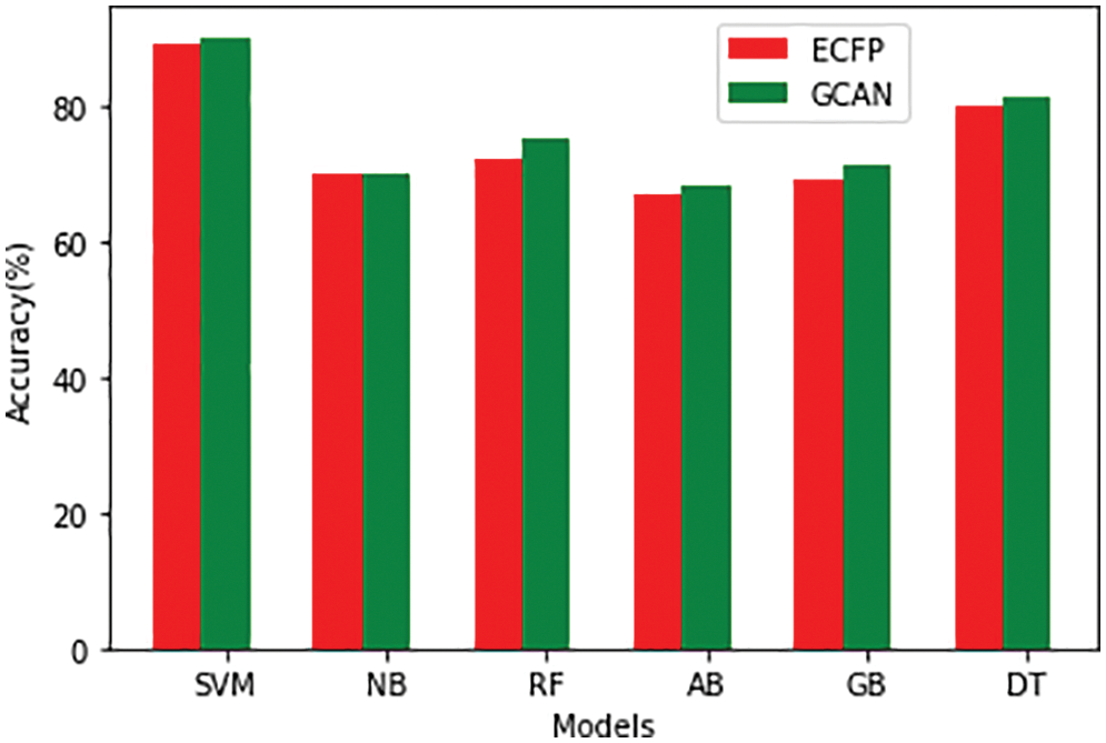
Figure 7: Accuracy

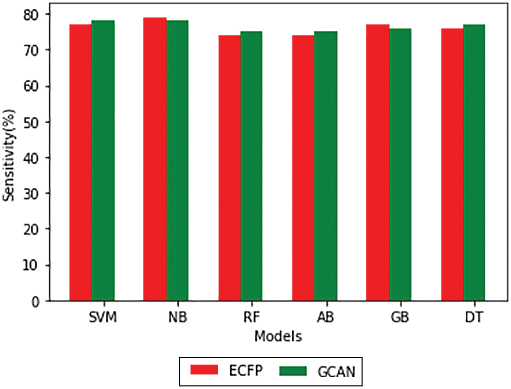
Figure 8: Sensitivity

Figure 9: Specificity

Table 3 compares our GCAN molecular fingerprint with the ensemble stacking model to known literature approaches. The proposed method has 91.6 percent accuracy, which is higher than other current methods. It has a specificity of 91% and a sensitivity of 89.5%, which is higher than any other model. The specificity and area under the curve of our proposed and Feng et al. are nearly identical, but our proposed method outperforms Feng et al. in terms of accuracy. It is due to the attention convolutional layer and the attention polling layer, which may obtain information from individual nodes and provide an aggregation from all hops.

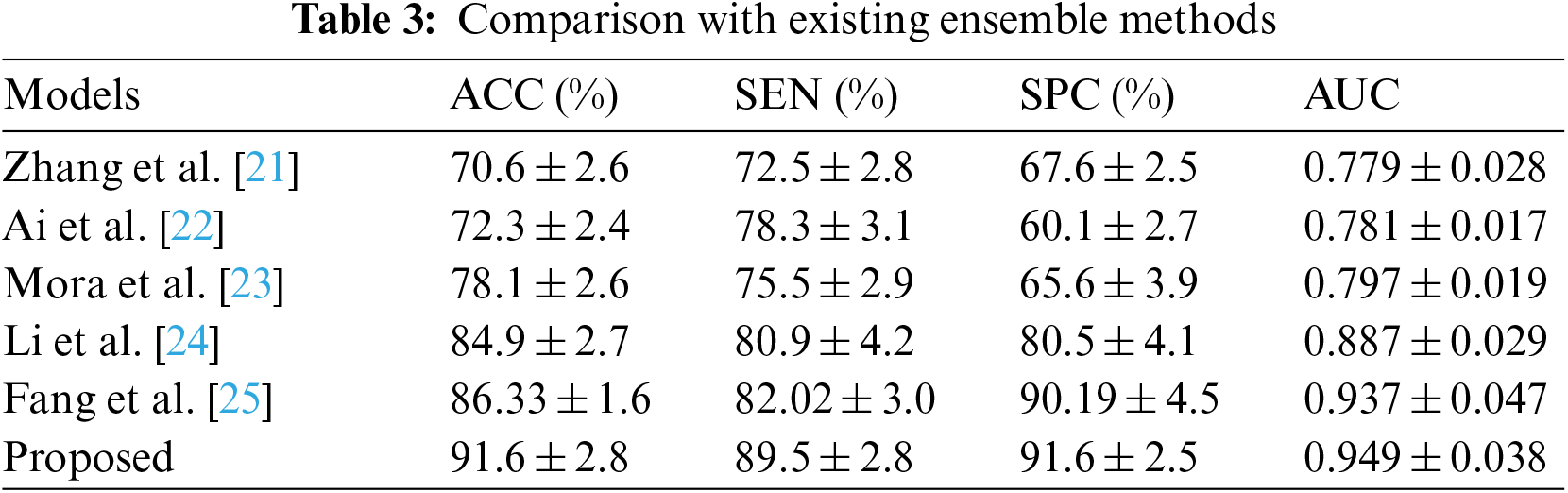
The ensemble model with the GCAN molecular fingerprint produces better results, as illustrated in Figs. 10–12. The distribution of valuable nodes is dynamically learned through attention pooling. GCAN can obtain more information underneath the graph input by employing an attention strategy to aggregate distinct hop neighbors. Without losing any individual node or global topology information, GCAN can collect a large number of graph signatures on the run. The GCAN over graph network proposes prominent advantages over deep learning approaches. GCAN is the most practical graph classification, even if graph neural networks still dominate the field. This is due to GCAN’s ability to handle efficiency and a variety of other issues that most graph networks encounter.

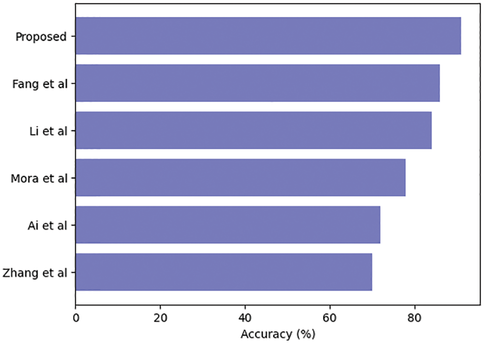
Figure 10: Ensemble model accuracy comparison

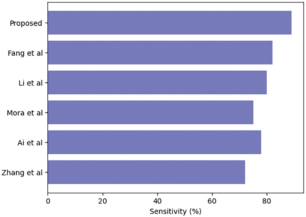
Figure 11: Ensemble model sensitivity comparison

Figure 12: Ensemble model specificity comparison

5  Conclusion

A drug classification model is proposed in this article that uses Graph Convolutional Attention Network (GCAN) to represent the drug as a molecular fingerprint representation, followed by an ensemble stacking model for classification. As base learners in stacking, SVM, Random Forest, Nave Bayes, Decision Tree, AdaBoost, and Gradient Boosting are employed. When it comes to typical GCN models, information is lost in every convolution step. We used an attention method to solve this problem. Our attention convolution layer architecture captures more hierarchical structure information than previous models, resulting in a more accurate representation of both individual nodes and the network as a whole. A self-attention mechanism is used by the attention pooling layer to focus on different features of the graph, resulting in a fixed-size, comprehensive graph representation matrix. The experimental results revealed that our proposed method has a higher accuracy of 91.6 percent which is better than previous methods. Furthermore, GCAN fingerprints provide superior representation when compared to other fingerprint representations. In future work, we intend to integrate a deep-learning classification model to classify more complex drug components.

Acknowledgement: The authors declare that they have no acknowledgement to report regarding the present study.

Funding Statement: The authors received no specific funding for this study.

Author Contributions: All authors are contributed equally to this work.

Availability of Data and Materials: This article does not involve data availability and this section is not applicable.

Conflicts of Interest: The authors declare that they have no conflicts of interest to report regarding the present study.

References

1. M. Butkiewicz, Y. Wang, S. H. Bryant, E. W. Lowe, D. C. Weaver et al., “High-throughput screening assay datasets from the pubchem database,” Chemical Informatics, vol. 3, no. 1, pp. 1, 2017. [Google Scholar] [PubMed]

2. J. Fayyad, M. A. Jaradat, D. Gruyer and H. Najjaran, “Deep learning sensor fusion for autonomous vehicle perception and localization,” Sensors, vol. 20, no. 15, pp. 4220, 2020. [Google Scholar] [PubMed]

3. L. Deng and X. Li, “Machine learning paradigms for speech recognition: An overview,” IEEE Transactions on Audio, Speech, and Language Processing, vol. 21, no. 5, pp. 1060–1089, 2013. [Google Scholar]

4. O. Braga and O. Siohan, “A closer look at audio-visual multi-person speech recognition and active speaker selection,” in ICASSP 2021 IEEE Int. Conf. on Acoustics, Speech and Signal Processing (ICASSP), Toronto, Ontario, Canada, pp. 6863–6867, 2021. [Google Scholar]

5. S. Morgan, P. Grootendorst, J. Lexchin, C. Cunningham and D. Greyson, “The cost of drug development: A systematic review,” Health Policy, vol. 100, no. 1, pp. 4–17, 2011. [Google Scholar] [PubMed]

6. J. Bajorath, “Integration of virtual and high-throughput screening,” Nature Reviews Drug Discovery, vol. 1, no. 11, pp. 882–894, 2002. [Google Scholar] [PubMed]

7. J. S. Mason, A. C. Good and E. J. Martin, “3-D pharmacophores in drug discovery,” Current Pharmaceutical Design, vol. 7, no. 7, pp. 567–597, 2001. [Google Scholar] [PubMed]

8. V. J. Gillet, P. Willett and J. Bradshaw, “Similarity searching using reduced graphs,” Journal of Chemical Information and Computer Sciences, vol. 43, no. 2, pp. 338–345, 2003. [Google Scholar] [PubMed]

9. P. C. Hawkins, A. G. Skillman and A. Nicholls. “Comparison of shape-matching and docking as virtual screening tools,” Journal of Medicinal Chemistry, vol. 50, no. 1, pp. 74–82, 2007. [Google Scholar] [PubMed]

10. M. Totrov, “Atomic property fields: Generalized 3D pharmacophoric potential for automated ligand superposition, pharmacophore elucidation and 3D QSAR,” Chemical Biology & Design, vol. 71, no. 1, pp. 15–27, 2008. [Google Scholar]

11. R. Sivakumar, P. Sinha and V. Bharghavan, “CEDAR: A core extraction distributed ad hoc routing algorithm,” IEEE Journal on Selected Areas in Communications, vol. 17, pp. 1454–1465, 2002. [Google Scholar]

12. S. Singh, M. Woo and C. S. Raghavendra, “Power aware routing in mobile ad hoc networks,” in Proc. of IEEE Int. Conf. on Mobile Computing and Networking, Seattle, Washington, pp. 181–190, 1998. [Google Scholar]

13. R. Zheng and R. Kravets, “On demand power management for ad hoc networks,” Ad Hoc, vol. 3, pp. 51–68, 2005. [Google Scholar]

14. J. H. Chang and L. Tassiulas, “Energy conserving routing in wireless adhoc network,” in IEEE Int. Conf. on Computer Communications, Tel Aviv, Israel, vol. 1, pp. 22–31, 2000. [Google Scholar]

15. S. Kanakala, V. R. Ananthula and P. Vempaty, “Energy-efficient cluster based routing protocol in mobile ad hoc networks using network coding,” Journal of Computer Networks and Communications, vol. 2014, no. 351020, pp. 12, 2014. [Google Scholar]

16. B. E. Boser, I. M. Guyon and V. N. Vapnik, “A training algorithm for optimal margin classifiers,” in Proc. of the Fifth Annual Workshop on Computational Learning Theory, pp. 144–152, 1992. [Google Scholar]

17. D. D. Lewis, “Naive (Bayes) at forty: The independence assumption in information retrieval,” in European Conf. on Machine Learning, pp. 4–15, 1998. [Google Scholar]

18. L. Breiman, “Random forests,” Machine Learning, vol. 45, pp. 5–32, 2001. [Google Scholar]

19. Y. Freund and R. E. Schapire, “A Decision-theoretic generalization of on-line learning and an application to boosting,” Journal of Computer and System Sciences, vol. 55, pp. 119–139, 1997. [Google Scholar]

20. S. L. Salzberg, “C4.5: Programs for Machine Learning” J. Ross Quinlan Morgan Kaufmann Publishers, pp. 235–240, 1994. [Google Scholar]

21. L. Zhang, H. Ai, W. Chen, Z. Yin, H. Hu et al., “CarcinoPred-EL: Novel models for predicting the carcinogenicity of chemicals using molecular fingerprints and ensemble learning methods,” Scientific Reports, vol. 7, no. 1, pp. 1–14, 2017. [Google Scholar]

22. H. Ai, W. Chen, L. Zhang, L. Huang, Z. Yin et al., “Predicting drug-induced liver injury using ensemble learning methods and molecular fingerprints,” Toxicological Sciences, vol. 165, pp. 100–107, 2018. [Google Scholar] [PubMed]

23. J. R. Mora, Y. Marrero-Ponce, C. R. García-Jacas and A. Suarez Causado, “Ensemble models based on QuBiLS-MAS features and shallow learning for the prediction of drug-induced liver toxicity: Improving deep learning and traditional approaches,” Chemical Research in Toxicology, vol. 33, pp. 1855–1873, 2020. [Google Scholar] [PubMed]

24. S. Kwon, H. Bae, J. Jo and S. Yoon, “Comprehensive ensemble in QSAR prediction for drug discovery,” BMC Bioinformatics, vol. 20, pp. 1–12, 2019. [Google Scholar]

25. M. Liu, L. Zhang, S. Li, T. Yang, L. Liu et al., “Prediction of hERG potassium channel blockage using ensemble learning methods and molecular fingerprints,” Toxicology Letters, vol. 332, pp. 88–96, 2020. [Google Scholar] [PubMed]

26. Y. Sicak, “Synthesis, predictions of drug-likeness, and pharmacokinetic properties of some chiral thioureas as potent enzyme inhibition agents,” Turkish Journal of Chemistry, vol. 46, no. 3, pp. 665–676, 2022. [Google Scholar] [PubMed]

27. K. Lee, J. Jang, S. Seo, J. Lim and W. Y. Kim, “Drug-likeness scoring based on unsupervised learning,” Chemical Science, vol. 13, no. 2, pp. 554–565, 2022. [Google Scholar] [PubMed]

28. C. Kurapati, K. Paidikondala, V. N. Badavath, S. Parveen, O. V. Singh et al., “Design, and synthesis of N-benzyl spiro-piperidine hydroxamic acid-based derivatives: Histone deacetylase inhibitory activity and drug-likeness prediction,” Journal of Heterocyclic Chemistry, vol. 59, no. 11, pp. 2006–2015, 2022. [Google Scholar]

29. G. Singh, A. Singh, S. Singh, Y. Thakur, K. N. Singh et al., “Design, synthesis, drug-likeness and in silico prediction of polycyclic aromatic schiff base tethered organosilatranes,” Silicon, pp. 1–7, 2022. [Google Scholar]

30. A. Tafida, I. M. Tukur, S. G. Adamu, U. A. Bello and T. A. Salisu, “Molecular docking simulation, pharmacokinetic and drug-likeness properties prediction of some flavanoid derivatives as anti cholerae agents,” ATBU Journal of Science, Technology and Education, vol. 9, no. 4, pp. 190–198, 2022. [Google Scholar]