Physics Based Digital Twin Modelling from Theory to Concept Implementation Using Coiled Springs Used in Suspension Systems

Nomenclature

1  Introduction

The new industrial revolution considered industrial 4.0, where the systems used in manufacturing operations are integrated with the information and communication technologies (ICT). At this stage, the Cyber-Physical Systems (CPS) formed based on the advent of the materials and capabilities of the sensor. In other words, the IoT became the backbone of the fourth industrial revolution [1]. This industrial revolution changed how models behave in companies, businesses, and academia; the competition rules adapted to the IoT ideas and concepts. IoT pushed the Industrial Revolution further to the digitalization stage [2]. From the industrial point of view, digital technology solutions offer better opportunities for industrial companies and consumers, saving time, reducing unnecessary costs, reducing downtime, and increasing the availability of services [3]. In 2002, Michael Grieves introduced the term “(Digital Twin)” for the first time; of course, the proposal was in the context of Product Lifecycle Management (PLM) [4].

According to the Whitepaper, which was written by Grieves in the same year [5] defined DT as a replication of the actual physical system, and he stated three dimensions for this replication (A) Physical entity (B) Digital counterpart (C) Connection between physical and digital. However, this was not a formal definition. Even though the concept of digitalization existed much longer before Grieves was introduced, the term DT itself was the first time Grieves mentioned it in 2002. In 2010 NASA defined DT in the context of modelling, simulation, information technology and processing roadmap [6]. Between 2005 and 2010, many technical improvements were introduced; NASA and the US Air Force included DT in the aircraft’s structural management of planes. The definition of the DT presented by Grieves is unclear and confusing. Many industries and researchers still use different technologies and name them DTs while they are not. This digital twining revolution has to consider Industrial 5.0 because it has advanced dimensions from Industry 4.0 [7]; however, the DT needs standardization first. Additionally, the standardization stops industries and academics from using industrial 4.0 technologies such as IoT and, name it DT, putting the DT technology in danger of reaching the plateau.

1.1 Characteristics DT Technology

In the enthralling nexus of smart technologies, such as integrating AI with DTs emerges as a paradigm that exemplifies technological synergy, steering unprecedented advancements across myriad sectors as shown in Fig. 1. As virtual replicas of physical entities or systems, DTs interactively mirror RT conditions and changes, while AI introduces the capabilities of learning, reasoning, and self-correction to this dynamic digital replica. This amalgamation brings about enhanced predictive maintenance and operational efficiency and pioneers intelligent decision-making and autonomous actions in the digital replica.

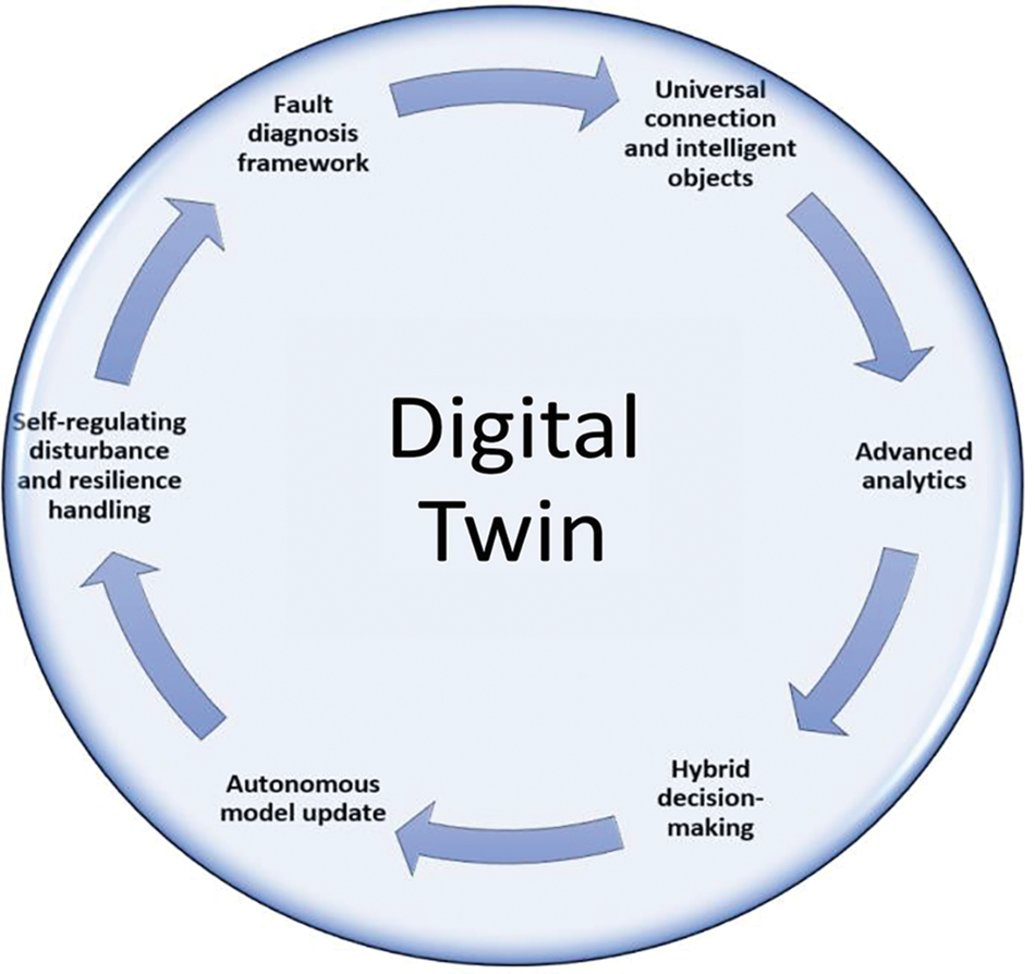
Figure 1: The overall characteristics of digital twins

A) Universal connection and intelligent objects: The manufacturing equipment should be outfitted with smart sensors capable of RT monitoring and data exchange with other network elements. A risk-free, dependable, quick platform must accommodate these nonstop data exchanges.

B) Advanced analytics: It is necessary to automate as much of the data preparation, perception, analysis, learning, and execution process as possible while minimizing the amount of manual feature engineering and human intervention. It is now possible for production systems to self-configure, self-adapt, and self-learn, increasing productivity, speed, flexibility, and efficiency [8].

C) Hybrid decision-making: RT data limitations and data from many sources must be considered to arrive at a globally optimal solution. Several orders will have their practicability, efficacy, and efficiency regarding implementation methodologies reviewed during this procedure [9].

D) Autonomous model update: RT control, optimization, forecasting, and other similar activities necessitate the synchronization of data and the use of complex modeling techniques to map between VS and PS.

E) Self-regulating disturbance and resilience handling: Smart robots are interdisciplinary technology that integrates sensing and analyzing production information, representation of experience, and knowledge. One of the features of smart robots is intelligent decision-making based on information, data, experience, and prior knowledge. It can simulate, model, and autonomous operation.

F) Fault diagnosis framework: DTs are a living representation of a physical system backed by multi-physics simulation, machine learning, AR/VR, and cloud services. These multi-physics support results and enable constant environmental or operational adjustments for DTs [10].

1.1.1 Models

Throughout the lifecycle of any physical object in the real world, it is crucial to have its model in the digital world mirror each other continuously. The digital model consists of different models to visualize the physical object in 3D in the virtual world. Models are a critical part of DT as they are the initial step in developing or creating a twin for the physical object in the digital world. They provide a complete and detailed reflection of the physical object and insight into it through simulations. However, as the data have been gathered and combined through people, information systems, and sensors, the models themselves will have a specific function; these functions can be summarised as follows: (A) reproduction of rules, behaviors, and properties for the physical object (B) the autonomous operation in the virtual space (C) the prediction of issues before its occurrence (D) development of preventive strategies (E) performance validation.

1.1.2 Data

Data is the brain that makes DT work, which provides intelligence to operate DT continuously. Data come from virtual and physical spaces; virtual space provides data from simulations and information systems. All the data combined to give the driver for the DT through big data analytics deals with a large and diverse set of data. Where valuable information can be minded and unnecessary data can be ignored. Data play a vital role as a full DT version of the physical object cannot work without it.

1.1.3 Connections

The ability to connect is essential for the creation of a digital twin. Using this technology can connect a physical element to its digital counterpart. By gathering, integrating, and transferring data through various integration methods, sensors make it possible to connect physical objects. Integrating the physical and virtual space is critical and completes the cycle between the model and the physical object. Connections are essential to bringing every element in every entity to live in the DT. However, connections can be divided into three categories as follows: (A) connection within the physical space, where the entities are interconnected for data exchange (B) connection within virtual space, where the model and information systems are interconnected (C) connection between the physical and virtual space, where the entities are linked with the corresponding virtual objects to provide a closed-loop for the sensing and control. The achievement of this comprehensive connection will provide an iterative optimization throughout the lifecycle of the products.

1.1.4 Services

Services are the final form in which DT can be presented with, or is the user interfaces where the standard formats of functions can be visible to the user, such as input, output, and primary and standard information to communicate with the virtual and physical spaces. Services like the black boxes are used without knowing the internal mechanisms, all the users do, provide the input parameters and request the output. Services accessed with a bit of professional understanding simplify and ease DT usage and expand the DT applications to more user groups. Since many authors still assume that the DT is collected during product development, from digital artifacts to the collected data during product use; therefore, this paper proposes a novel concept for the DT. The idea or definition introduced by this paper is that the “DT is a Live virtual replica that continuously simulates the entire mechanical behavior of anything”, where the replication must mirror the entire internal and external mechanical behavior. This concept is suitable for both industries and academics. When used, for example, the entire representation of the thing in maintenance will represent the systems’ current real-time mechanical behavior. Still, it will also diagnose both electrical and mechanical faults and classify them. For this study, this paper, for the first time, validated the proposed concept using Euler’s method to replicate the entire mechanical behavior of a coil spring used in many systems through all industries and studies.

1.2 Aim of the Study

This study aims to conceptualize the Digital Twin (DT) technology. The idea introduced in this study is cost-effective and straightforward to implement in both industry and academia. While the aim is only to conceptualize the DT, the mechanical behavior of the coil spring is used to validate the proposed concept based on Euler’s method.

1.2.1 Conceptualising Digital Twin

This study aims to conceptualize the DTs and prove that the DT mode can provide more accurate results similar to the experimental ones by analyzing the mechanical structure of coil springs used in suspension systems with the current time data flow, which eventually provides safety within automated mechanical systems by diagnosing faults and their classification.

The rest of this paper is organized as follows: Section 2 describes the related work, Section 3 describes the materials used and methodology, Section 4 describes results and discussion and Section 5 describes conclusion.

2  Related Work

The workshop of “Dartmouth Summer Research Project”, which was organized by John McCarthy in 1956 on Artificial Intelligence (AI), now is considered by many to be the official declaration of as a research field in the AI [11]. The research in AI since 1956 developed intelligent systems, that not only doing physical work but also is capable of reasoning and predicting future events, hence decision making. With the advent of Machine Learning (ML), Deep Learning (DL), Central Processing Unit (CPU), Graphics Processing Unit (GPU), Tensor Processing Unit (TPU) and computational power, the applications of AI are involved as an essential part of our daily life.

In 1970, NASA was the first to generate the concept of the (physical twin) through system engineering and condition monitoring, in Apollo 13, two identical spaceships were created, one of which was launched in space to perform the mission and remained on Earth. NASA used the one that remained on the ground to analyze what was happening in the area [12]. They understood the digital twin technology phenomenon and immediately investigated its impact on business [13]. Digital twin technologies have gained wide publicity; however, despite the significant work done and discovery that promises a prospering future in integrating digital twins in industries, the state of the research is not transparent [14]. The concept is not well understood, which impacts the future development of technology. Therefore, a well-established literature review methodology is in line with [15].

2.1 Theoretical DT Concepts

Since 2016, there has been an overwhelming number of publications on DTs, however, none comprehensively review DTs. Some of the most important ones are summarised below. Following this, institutions and scholars submitted their definitions of DTs, including extensive and varied precise descriptions. It depends on the research as long as the report covers the three critical aspects of Grieves’ framework [13]. Table 1 summarises the concepts of DTs found in the literature.

2.2 Platforms for the DT Technologies Development

DT technology is becoming one of the most promising technologies in all industries. The railway industry is not included in this study simply because it is one of the few industries which did not take full advantage of the DT technology. As shown in Table 2, numerous organisations provide different tools and software for DTs to visualise actual products and increase business through various industry sectors.

3  Methodology

This section covers the analytical and numerical solutions (Euler method) for the main parameters that characterize the behavior for the different constructed vibration systems. The analysis is subject to the other operating conditions, incorporating the output responses, strains, normal, maximum induced shear, and shear Von-mises stress within the oscillating spring, the spring’s properties are shown in Table 3. Two central vibration systems included throughout this section are (i) linear and (ii) non-linear systems. These two cases involve undamped (i) and (ii) damped cases. Each one of the mentioned cases is subjected to three different conditions, which are (i) Free-Vibration (in the absence of the applying external force), (ii) Steady-Forced Vibration and (iii) Transient-Forced Vibration.

3.1 Linear Vibration Systems (Undamped)

This section investigates the analytical solutions for the output response, normal strain, normal and maximum induced shear stress within each of the three different linear-vibration operating conditions as a function of time in detail, where the damping effect is ignored.

3.1.1 Free-Vibration System

Fig. 2A displays the construction of a simple free-vibration system (where the weight of an oscillating object and damping forces are not considered), consisting of the spring and the object. The figure shows that the object was displaced by an amplitude initially, where the general expression for the displacement of an oscillating object concerning the time, defined as follows:

my(t)¨+ky(t)=0(1)

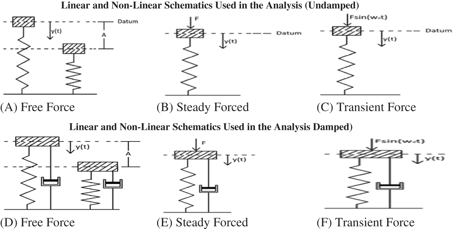
Figure 2: Shows the schematics used in the analysis from (A) to (F)

Therefore, the displacement y(t) based on the above equation obtained as follows:

y(t)=Acos(ωnt)(2)

ωn illustrates the natural frequency of the system, obtained from the following equation:

ωn=km(3)

where m and k denote for the mass of an oscillating object and the stiffness (spring rate) of the spring within the system, the expressions for the generated normal strain, normal stress and the maximum induced shear stress for all cases concerning the time based on the above-system are stated as follows:

ε=y(t)Lf(4)

σ=4ky(t)πd2(5)

τmax=Ks8ky(t)dπD3(6)

Ks=4C−14C−4+0.615C(7)

C=D2d(8)

3.1.2 Steady Forced-Vibration System

Fig. 2B illustrates the forced vibration oscillation system, where the steady external force is applied at an oscillating object. Therefore, it is the corresponding displacement would be defined as follows:

my(t)¨+ky(t)=−F(9)

The corresponding expression for the displacement of Eq. (9) would be:

y(t)=−Fk(1−cos⁡(ωnt))(10)

3.1.3 Transient Forced-Vibration System

Fig. 2C represents the transient forced-vibration oscillation system, where the external transient force is applied at an oscillating object. Therefore, the equation of the motion that describes the above figure would be:

my(t)¨+ky(t)=−Fsin(ωdt)(11)

Since ωd Indicates the driving frequency of the system; therefore, a general analytical solution for the displacement of this system concerning the time and the given driving frequency calculated from the following:

y(t)=Fm(ωn2−ωd2)(ωdωnsin⁡(ωnt)−sin⁡(ωdt))(12)

3.2 Linear Vibration Systems (Damped)

This section examines the analytical solutions for the output response, normal strain, normal and maximum induced shear stress within each of the three different linear-vibration operating conditions as a function of time in detail, and the damping effect.

3.2.1 Free-Vibration System

Fig. 2D shows the construction of a simple free-vibration system consisting of the spring, damper and object. The following equation of motion characterises this system:

my(t)¨+cy˙(t)+ky(t)=0(13)

Based on the initial conditions where at t=0, y=A and y˙=0, general expressions for the displacement of an oscillating object-based, assuming its corresponding response is underdamped (ξ < 1) would be:

y(t)=Ae−ξωntcos⁡(ωat)(14)

where ξ and ωa denote for the damping ratio and actual frequency of an oscillating object within the system, determined from the following:

ξ=caccr=ca4mk(15)

ωa=ωn1−ξ2(16)

3.2.2 Steady Forced-Vibration System

Fig. 2E illustrates a steady forced vibration oscillation system, including the damping effect. The next model attributes the equation of motion for this system:

my(t)¨+cay˙(t)+ky(t)=−F(17)

By using the initial conditions at t=0, y=0 and y˙=0, a general expression for an output response of an oscillating object for this given system obtained as follows:

y(t)=Fk(ξωnωae−ξωntsin⁡(ωat)+e−ξωntcos⁡(ωat)−1)(18)

3.2.3 Transient Forced-Vibration System

Fig. 2F displays the transient forced-vibration oscillation system, where the opted external transient force is applied at an oscillating object. The equation of motion is given as follows:

my(t)¨+cy˙(t)+ky(t)=−Fsin(ωdt)(19)

Initial conditions of the steady-forced vibration system are applied to obtain the following expression of the object’s displacement.

y(t)=B1e−ξωnt(B1cos⁡(ωat)+B2sin(ωat))+X0sin(ωdt−∅)(20)

where B1, B2, X0 and ∅ are defined as follows:

B1=X0sin⁡(∅)(21)

B2=X0ωdsin⁡(∅)−B1ξωnωa(22)

X0=(−F/k)((1−(ωdωn)2)2+(2ξωdωn)2)12(23)

∅=tan−1(2ξωd/ωn1−(ωdωn)2)(24)

3.3 Non-Linear Vibration Systems (Undamped)

This section studies the analytical solutions for the output response, normal strain, normal and maximum induced shear stress for the non-linear vibration system, consisting of four springs under three different operating conditions, excluding the damping effects throughout all the segments.

3.3.1 Free-Vibration System

Fig. 2A represents the construction of the non-linear free-vibration system, composed of four springs and objects.

Determining the natural frequency for the system is shown in Fig. 2A.

The equations of motion at node 1 within the system would be:

my¨1(t)=−k1(y1(t)−y2(t))(25)

my¨1(t)=−k1(y1(t)−y2(t)), my¨1(t)+k1(y1(t)−y2(t))=0(26)

The equation of motion at node 2

k1(y1(t)−y2(t))=k2(y2(t)−y3(t))(27)

The equation of motion at node 3

k2(y2(t)−y3(t))=k3(y3(t)−y4(t))(28)

The equation of motion at node 4

k3(y3(t)−y4(t))=k4y4(t)(29)

Since no damping is taking place throughout the entire system, an expression that associates the displacements y1, y2, y3 and y4 is given below:

keqy1(t)=k1(y1(t)−y2(t))=k2(y2(t)−y3(t))=k3(y3(t)−y4(t))=k4y4(t)(30)

Using the relationships given in Eq. (30) to obtain the following matrix:

[m000000000000000][y¨1y¨2y¨3y¨4]+[k1−k100−k1k1+k2−k200−k2k2+k3−k300−k3k3+k4][y1y2y3y4]=[0000](31)

Using the initial conditions at

y˙3=0,y4=A4 and y˙4=0, where A1, A2, A3 and A4 are the initial displacements (amplitude) of the nodes. Based on the equations mentioned above, the proposed analytical expressions for the displacements of nodes y1, y2, y3 and y4 would be as follows:

y1(t)=A1cos(ωxt)(32)

y2(t)=A2cos(ωxt)(33)

y3(t)=A3cos(ωxt)(34)

y4(t)=A4cos(ωxt)(35)

Using the Eqs. (32)–(35) and associating them with the matrix relationship illustrated in Eq. (32) to obtain the following matrix relationship:

[k1−mωx2−k100−k1k1+k2−k200−k2k2+k3−k300−k3k3+k4][A1A2A3A4]=[0000](36)

Taking the determinant of the square matrix Eq. (36) and equate it to zero to obtain the eigenvalue (square of natural frequency)

|k1−mωx2−k100−k1k1+k2−k200−k2k2+k3−k300−k3k3+k4|=0(37)

Based on the further derivation from the above determinant matrix, the expression for the ωx2 (eigenvalue) is obtained as follows:

ωx2=k1m(1+|−k1−k200k2+k3−k30−k3k3+k4||k1+k2−k20−k2k2+k3−k30−k3k3+k4|)=keqm(38)

keq is the equivalent spring rate of the entire system and obtained from the following relationship. Since the segments of the spring assumed connected in a series relationship:

1keq=1k1+1k2+1k3+1k4(39)

Therefore, the natural frequency of the system would be:

ωx2=(keqm)1/2(40)

Since it is a free vibration, therefore the initial displacement of node one can be decided or assumed, and by knowing this displacement at node 1 (A1) then the instantaneous displacements of nodes 2, 3, and 4 (A2, A3, A4) can be determined by making further derivation for Eq. (30) and further simplified by substituting some of the expressions obtained by X1, X2, and X3 as shown in Eqs. (41)–(43) to obtain instantaneous displacements of nodes 2, 3, and 4 (A2, A3, A4)

X1=k1−keqk1(41)

X2=k2X1−keqk2(42)

X3=keqk4(43)

A2=X1A1(44)

A3=X2A1(45)

A4=X3A1(46)

3.3.2 Steady Forced-Vibration System

Fig. 2B represents the non-linear vibration system, including the applying external steady force on the object. The equations of motion, including the oscillating object at node one, are expressed in the following equation from the above diagram.

my¨1(t)+k1(y1(t)−y2(t))=−F(47)

The equations of motion at nodes 2, 3, and 4 will be the same as expressed in the previous system from Eqs. (27)–(29). Since the initial displacements at nodes 1, 2, 3 and 4 taken to be zero at time zero, the analytical solutions for the displacements of y1, y2, y3 and y4 concerning the time can be derived using second-order differential equation between equations of motions expressed in Eqs. (27)–(29) and Eq. (47) to obtain the followings

y1(t)=(−Fkeq)(1−cos(ωxt))(48)

y2(t)=(−FX1keq)(1−cos(ωxt))(49)

y3(t)=(−FX2keq)(1−cos(ωxt))(50)

y4(t)=(−FX3keq)(1−cos(ωxt))(51)

3.3.3 Transient Forced-Vibration System

Fig. 2C represents the non-linear vibration system in applying external transient force on the object. The equations of motion of an oscillating object within the system would be:

my¨1(t)+k1(y1(t)−y2(t))=−Fsin(ωdt)(52)

The equations of motion at nodes 2, 3, and 4 will be the same as expressed in the previous system from Eqs. (27)–(29). Since the initial displacements at nodes 1, 2, 3 and 4 taken to be zero at time zero, the analytical solutions for the displacements of y_1, y_2, y_3 and y_4 concerning the time derived using second-order differential equation between equations of motions expressed in Eqs. (27)–(29) and Eq. (52) to obtain the followings.

y1(t)=(Fm((ωx)2−(ωd)2))((ωdωx)sin⁡(ωxt)−sin⁡(ωdt))(53)

y2(t)=(FX1m((ωx)2−(ωd)2))((ωdωx)sin⁡(ωxt)−sin⁡(ωdt))(54)

y3(t)=(FX2m((ωx)2−(ωd)2))((ωdωx)sin⁡(ωxt)−sin⁡(ωdt))(55)

y4(t)=(FX3m((ωx)2−(ωd)2))((ωdωx)sin⁡(ωxt)−sin⁡(ωdt))(56)

3.4 Non-Linear Vibration Systems (Damped)

This section studies the numerical solutions for the output response for the non-linear vibration system, consisting of three active springs under three different operating conditions, including the damping effect within the first spring only.

3.4.1 Free-Vibration System

Fig. 2D represents the construction of the non-linear free-vibration system, consisting of three active springs, object and damping throughout the first spring. The equation of motion of an oscillating object (node 1) within the system would be:

my¨1(t)+c1(y˙1(t)−y˙2(t))+k1(y1(t)−y2(t))=0(57)

The equation of motion at a junction point (node 2) between spring one and spring two within the system would be defined as follows:

c1(y˙1(t)−y˙2(t))+k1(y1(t)−y2(t))−c2(y˙2(t)−y˙3(t))−k2(y2(t)−y3(t))=0(58)

The equation of motion at a junction point between spring two and spring 3 (node 3) within the system is described as follows:

c2(y˙2(t)−y˙3(t))+k2(y2(t)−y3(t))−c3(y˙3(t)−y˙4(t))−k4(y3(t)−y4(t))=0(59)

The equation of motion at a junction point between spring three and spring four (node 4) within the system is described as follows:

c3(y˙3(t)−y˙4(t))+k3(y3(t)−y4(t))−c4y˙4(t)y4(t)=0(60)

Analytical solutions for y1, y2, y3 and y4 within Eqs. (57)–(60) concerning time cannot be achieved directly. Therefore, the numerical solutions for these displacements were obtained using Euler Method, taking initial conditions at t=0, y1=A1, y˙1=0, y2=A2, y˙2=0, y3=A3, y˙3=0, y4=A4, y˙4=0. The equation relationship is achieved by initially making the acceleration at node1(y¨1(t)) as a subject from Eq. (57).

y¨1(t)=−c(y˙1(t)−y2˙(t))−k1(y1(t)−y2(t))m(61)

To find the acceleration at node 1 (y¨1(t)) the values of the velocities at nodes 1 and 2 (y˙1(t) and y˙2(t)) and displacements at nodes 1 and 2 (y1(t) and y2(t)) must be known in advance, where the velocities are equal to zero at time zero. However, the displacements at time zero are equal to A1, and A2, respectively. Since the acceleration now is known, the Euler method is used to determine the velocity at node 1 in the following time step Δt explicitly.

y˙1(t)=y¨1(t−Δt)Δt+y˙1(t−Δt)(62)

Assuming the acceleration between the two-time steps is constant, the velocities in these two-time steps are known. Therefore, taking the average velocities and multiplying it by the change of time (time-step) will result in the change in displacement for node 1. Adding this change of displacement to the initial displacement will result in the displacement at the end of the given time-step. Therefore, the displacement y1(t) will be determined using the following:

y1(t)=(y˙1(t−Δt)+y˙1(t)+2)Δt+y1(t−Δt)(63)

By rearranging Eq. (58) to obtain the velocity at the node at two at a given time (t)

c1y˙2(t)+c2y˙2(t)=k1y1(t)+c1y˙1(t)+k2y3(t)+c2y˙3(t)−k1y2(t)−k2y2(t)(63*)

Making y˙2(t) as a subject from Eq. (58) to obtain the following equation:

y˙2(t)=k1y1(t)+c1y˙1(t)+k2y3(t)+c2y˙3(t)−k1y2(t)−k2y2(t)c1+c2(64)

Since the velocity at node two is known, then using the same technique as for node 1 to obtain the displacement at node two at a given time (t), which results in the following equation:

y2(t)=(y˙2(t−Δt)+y˙2(t)+2)Δt+y2(t−Δt)(65)

By rearranging Eq. (59) to obtain the velocity at node three at a given time (t)

c2y˙3(t)+c3y˙3(t)=k2y2(t)+c2y˙2(t)+k3y4(t)+c3y˙4(t)−k2y3(t)−k3y3(t)(65*)

Making y˙3(t) as a subject from Eq. (59) to obtain the following equation:

y˙3(t)=k2y2(t)+c2y˙2(t)+k3y4(t)+c3y˙4(t)−k2y3(t)−k3y3(t)c2+c3(66)

Since the velocity at node three is known, then using the same technique as for node 1 to obtain the displacement at node three at a given time (t), which results in the following equation:

y3(t)=(y˙3(t−Δt)+y˙3(t)+2)Δt+y3(t−Δt)(67)

By rearranging Eq. (60) to obtain the velocity at node four at a given time (t)

c3y˙4(t)+c4y˙4(t)=k3y3(t)+c3y˙3(t)−k3y4(t)−k4y4(t)(67*)

Making y˙4(t) as a subject from Eq. (60) to obtain the following equation:

y˙4(t)=k3y3(t)+c3y˙3(t)−k3y4(t)−k4y4(t)c3+c4(68)

Since the velocity at node four is known, then using the same technique as for node 1 to obtain the displacement at node four at a given time (t), which results in the following equation:

y4(t)=(y˙4(t−Δt)+y˙4(t)+2)Δt+y4(t−Δt)(69)

3.4.2 Steady Forced-Vibration System

Fig. 2E illustrates the same system as that for the bin non-linear free-vibration system, considering the applying external steady force on the object. The equation of motion of the constant forced oscillating object for node 1.

my¨1(t)+c1(y˙1(t)−y˙2(t))+k1(y1(t)−y2(t))=−F(70)

The equation of motion at nodes 2, 3 and 4 will be the same as mentioned in Eqs. (58)–(60). Going through the same procedure as that within the free-vibration system by determining the numerical solutions for the displacements y1, y2, y3 and y4 using Euler Method. The only difference between this system and the free-vibration system is the expression of y¨1(t) due to the inclusion of the steady external force, defined as follows:

y¨1(t)=−F−c(y˙1(t)−y2˙(t))−k1(y1(t)−y2(t))m(71)

3.4.3 Transient Forced-Vibration System

Considering the transient forced-vibration system will lead to the following equation of motion of a steady forced oscillating object within the system would be:

my¨1(t)+c1(y˙1(t)−y˙2(t))+k1(y1(t)−y2(t))−Fsin(ωdt)(72)

The equation of motion at nodes 2, 3 and 4 will be the same as mentioned in Eqs. (58)–(60). Going through the same procedure as that within the free-vibration system by determining the numerical solutions for the displacements y1, y2, y3 and y4 using Euler Method. The only difference between this system and the free-vibration system is the expression of y¨1(t) due to the inclusion of the transient external force, defined as follows:

y¨1(t)=−Fsin(ωdt)−c(y˙1(t)−y2˙(t))−k1(y1(t)−y2(t))m(73)

4  Results and Discussion

4.1 Linear Steady-Forced Vibration Systems (Undamped)

This section investigates the analytical solutions for the output response, normal strain, normal and maximum induced shear stress within each of the three different linear-vibration operating conditions as a function of time in detail, where the damping effect is ignored, as shown in Fig. 3.

Figure 3: Six resulting strain and stresses for linear steady-forced vibration system in the undamped scenario

4.2 Linear Transient-Forced Vibration Systems (Undamped)

It is noticed in Fig. 4 that the variations of the normal and maximum induced shear stress to behave similarly concerning the time is irregular compared to the behaviour of the linear-steady forced vibration system. Since Eq. (12) does not resemble the behaviour stated by Eq. (10) due to the inclusion of the driving frequency within the applying external force. Overall, the deflection and strain responses perform similarly to the stresses. Suppose the spring obeys isotropic behaviour. The given force and driving frequency of 1000 N and eight rad/s on the system led to the maximum normal and induced shear stress under these operating conditions: about 42.6 and 1251.35 MPa. This result characterises the spring’s failure due to induced shear stress since the shear yielding stress for this spring is about 410 MPa.

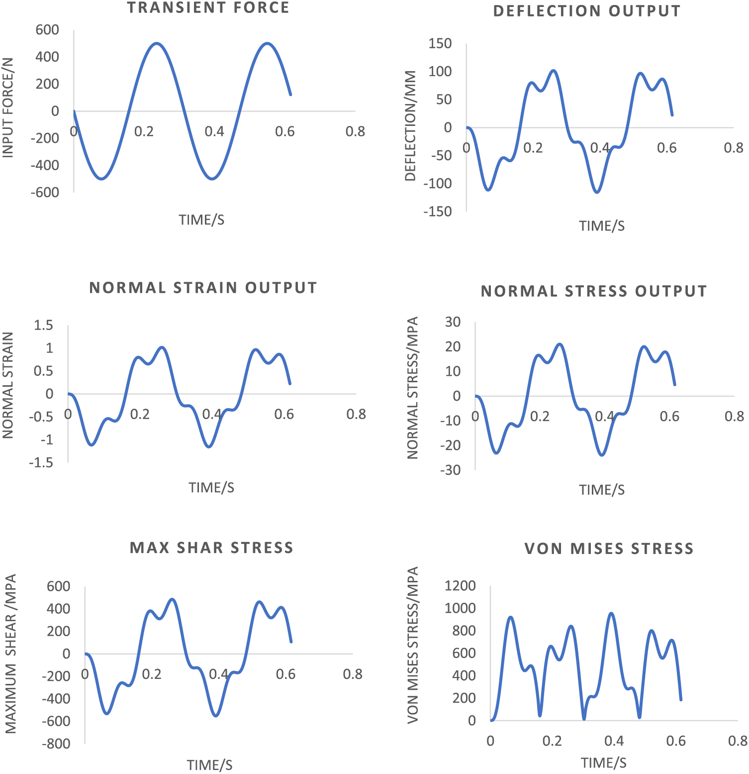
Figure 4: Six resulting strain and stresses for linear transient-forced vibration system in the undamped scenario

4.3 Linear Steady-Forced Vibration Systems (Damped)

According to Fig. 5, the damping effect considered, leading the variation of the stresses responses to get damped concerning the time compared to that described in Fig. 5, since the opted damping coefficient of the spring is lower than the critical damping of the entire system. Using the same given operating parameters as that provided within the undamped case (where applying steady force is 1000 N), and by taking the selected damping coefficient of the spring to be about 100 Ns/m, resulting in the obtained values for the maximum normal and induced shear stresses to be about −22.64 and −609 MPa. Once again, this signifies that failure would occur due to shearing mode since the obtained shear stress is greater than the shear yield stress.

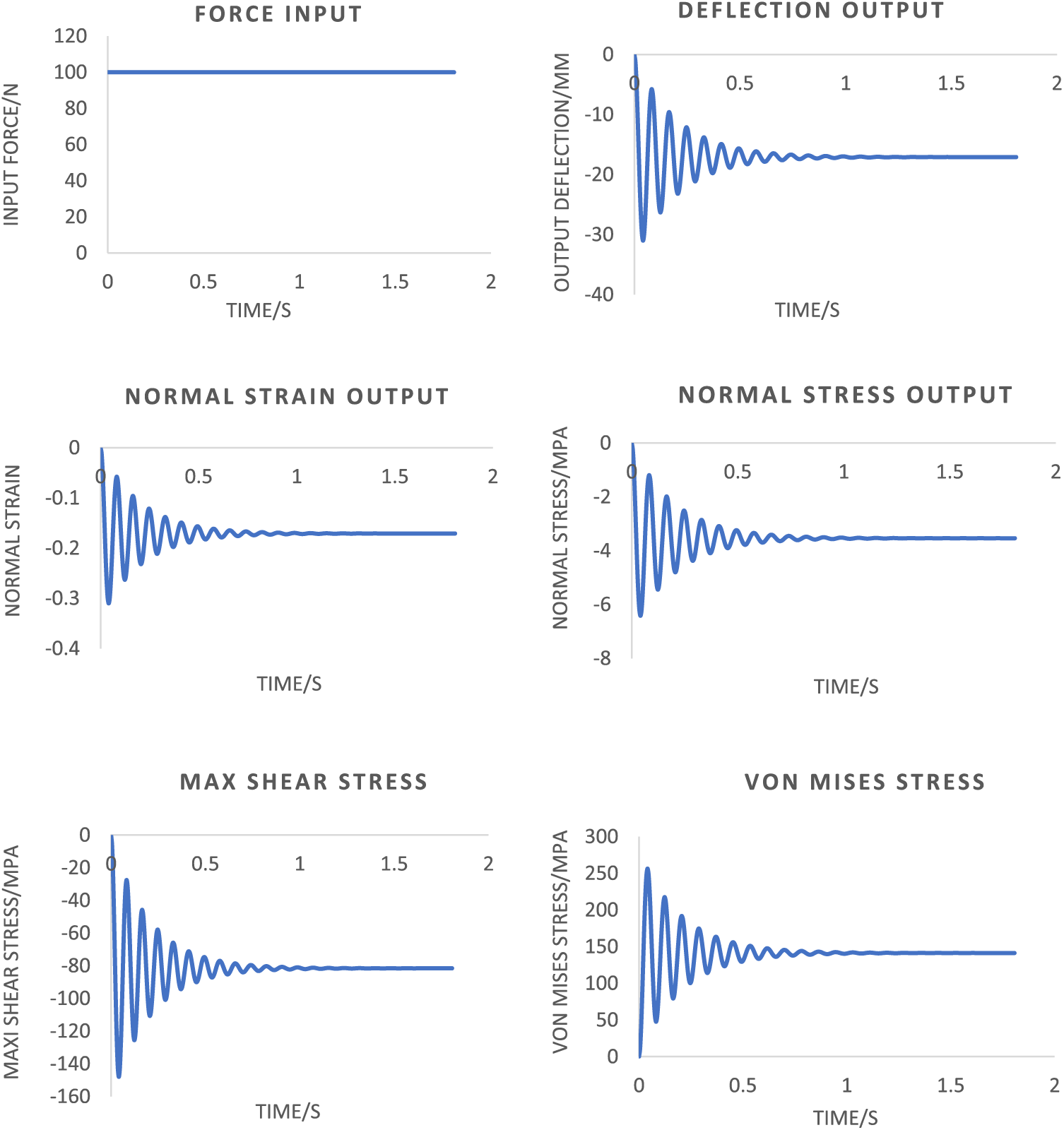
Figure 5: Six resulting strain and stresses for linear steady-forced vibration system in the damped scenario

4.4 Linear Transient-Forced Vibration Systems (Damped)

The damping effect into the system mentioned in the undamped linear transient-forced vibration system leads the output response slightly distorted compared to the rest of the spring’s motion within the first few seconds of the spring’s movement observed. The spring’s movement observation is interpreted as the transient response throughout this duration, which has gotten damped quite rapidly. The entire system’s overall response is the same as the steady-state response. Incorporating the damping effect into the system leads to the simple harmonic motion response. Using the same transient force, the undamped linear transient-forced vibration system has been mentioned. They obtained the maximum normal and induced shear stress values of about −14.78 and −433.90 MPa. Once again, this signifies that failure would occur due to shearing mode since the obtained shear stress exceeds the shear yield stress, as shown in Fig. 6.

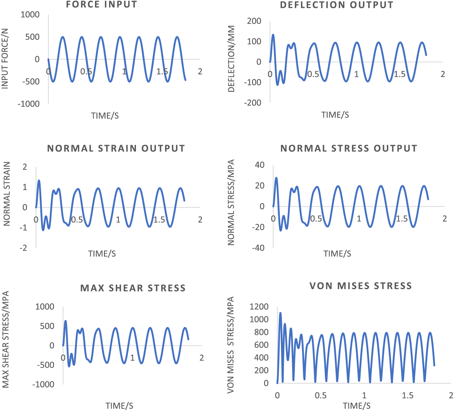
Figure 6: Six resulting strain and stresses for linear transient-forced vibration system in the damped scenario

4.5 Non-Linear Steady-Forced Vibration Systems (Undamped)

Fig. 7 shows the non-linear steady-forced vibration used in the un-damped case illustrates all measurements’ output response (deflection, strain, maximum normal and induced shear stresses). The output for each of the four springs behaves harmonically with the same natural frequency, with different values concerning the time due to the other geometric properties of each spring. Based on the assumption that all the springs within this vibration system obey the isotropic behaviour, and using the applying force of 1000 N, resulting they obtained values for the maximum normal and induced shear stresses to be about −70.02 and −2055.5 MPa for spring 1, −59.42 and −1744.06 MPa for spring 2, −101.86 and −2989.82 MPa for spring 3, −25.47 and −747.45 MPa for spring 4. These values indicate that springs 1, 2 and 3 will fail due to their high shear stresses (spring three will be the first among them), while spring four will be the least likely to fail since its shear stress has not yielded yielding shear stress.

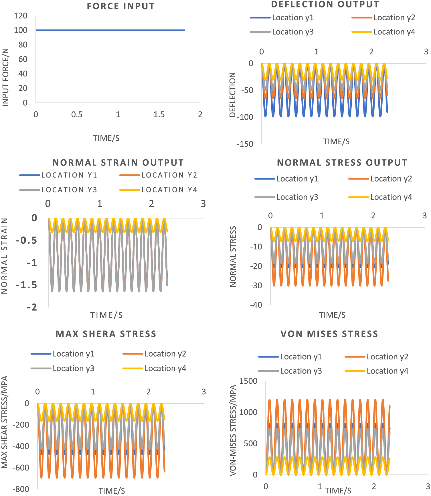
Figure 7: Six resulting strain and stresses for the non-linear steady-forced vibration system in the damped scenario

4.6 Non-Linear Transient-Forced Vibration Systems (Undamped)

Fig. 8 shows the non-linear transient vibration un-damped case shows the output response of all measurements (deflection, strain, maximum normal and induced shear stresses). The output for each of the four springs behaves with the same natural frequency, where the amplitude of each of the operating springs changes throughout their motions, since the type of the force acting on the oscillating object is transient force, incorporating the driving frequency parameter. Based on the selected value of 1000 N at a driving frequency of 8 rad/s, the resultant maximum normal and shear stresses are bout 70.66 and 2074.11 MPa, respectively. For spring 1, 59.96 and 1759.85 MPa for spring 2, 102.78 and 3016.89 MPa for spring 3, 29.69 and 754.22 MPa for spring 4. These values indicate that springs 1, 2 and 3 will fail due to their high shear stresses (where spring three will be the first among them), and spring 4 will be the least likely to fail since its shear stress has the lowest value among all the springs.

Figure 8: Six resulting strain and stresses for the non-linear transient-forced vibration system in the undamped scenario

4.7 Non-Linear Steady-Forced Vibration Systems (Damped)

The construction of this system would be similar to that mentioned within the section of the un-damped non-linear steady-forced vibration systems; the only difference is throughout the analysis of springs’ motions within the system, which is attached to the base neither gets extended nor gets compressed. From the theoretical studies section, where the numerical solutions using the Euler method for the displacements of y1, y2 and y3 Based on the given applying the steady force of 1000 N and a damping coefficient of 100 Ns/m (takes place only through the first spring). Therefore, this method leads the maximum generated normal and induced shear stresses within these springs are shown in Fig. 9.

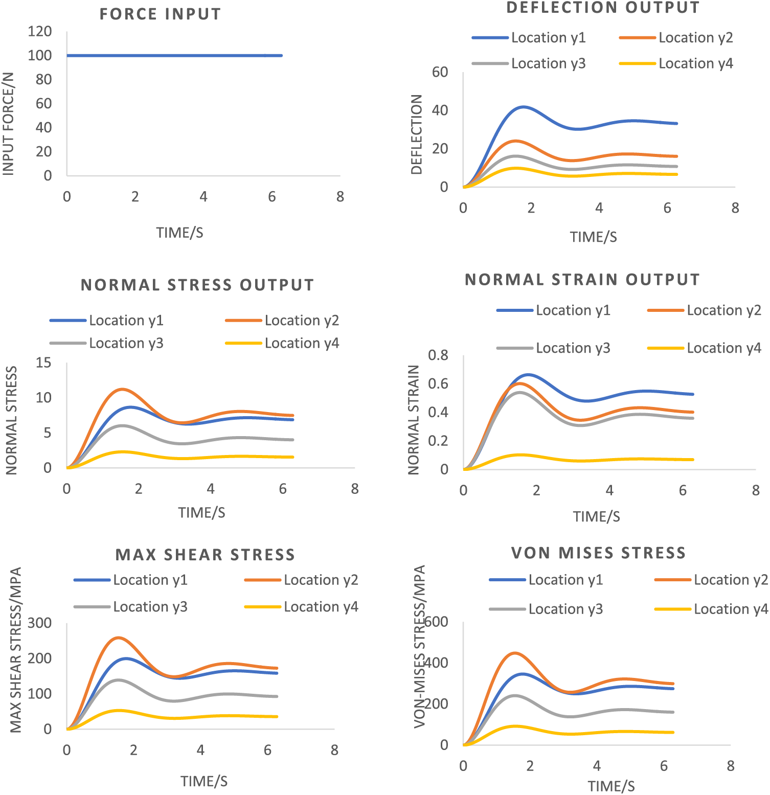
Figure 9: Six resulting strain and stresses for the non-linear steady-forced vibration system in the damped scenario

Spring 1: −50.62 MPa (Maximum Normal Stress) and −1485.7 MPa (Maximum induced shear stress). Spring 2: −33.80 MPa (Maximum Normal Stress) and −992.15 MPa (Maximum induced shear stress). Spring 3: −25.35 MPa (Maximum Normal Stress) and −744.11 MPa (Maximum induced shear stress). These values show that the shear failure would occur among all of these springs since their shear stresses exceeded the yielding shear stress.

4.8 Non-Linear Transient-Forced Vibration Systems (Damped)

Based on the system’s construction that comprises three active springs (as mentioned for damped non-linear steady-forced vibration system) and as shown in Fig. 10, and replacing the steady-force with the transient force having a magnitude of 1000 N with a driving frequency of 8 rad/s. The conditions mentioned lead the maximum generated normal and induced shear stresses (again based on the Euler Method) within these springs to be as follows: Spring 1: −153.227 MPa (Maximum Normal Stress) and −4497.58 MPa (Maximum induced shear stress). Spring 2: −101.57 MPa (Maximum Normal Stress) and −3010.01 MPa (Maximum induced shear stress). Spring 3: −76.91 MPa (Maximum Normal Stress) and −2257.51 MPa (Maximum induced shear stress). These values illustrate that the shear failure would occur among these springs since their shear stresses exceeded the yielding shear stress.

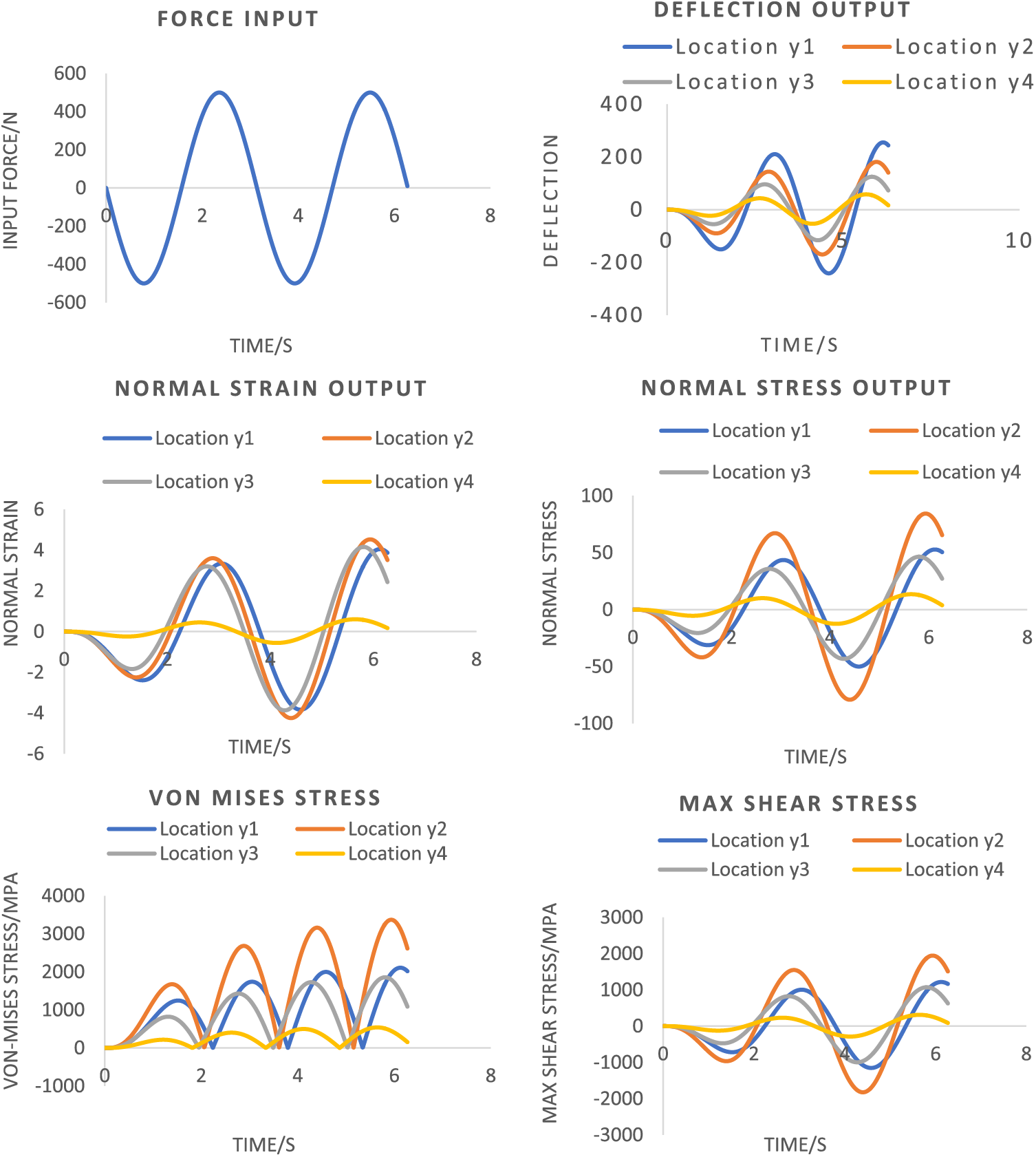
Figure 10: The resulting strain and stresses for the non-linear transient-forced vibration system in the damped scenario

4.9 Overall Stiffness Matrix

Table 4 shows the stiffens matrix for each coil in the spring, then adding them all to make the overall stiffness matrix.

4.10 Overall Compliance Matrix

Table 5 shows the overall compliance matrix by taking the inverse of the stiffness matrix, this will result in the compliance matrix.

4.11 Digital Twin Model (DTM)

The DT model shows the current real-time visual representation of the mechanical behaviour of the vibrating system (Coil Spring). This model is based entirely on only one input which is the load applied on the spring. Fig. 11 represents the physics-based discrete-time model, which provides a graphical representation of the current real-time mechanical behaviour of the vibrating system (more precisely, the Coil Spring). The load that is being applied to the spring is the sole input that this model takes into consideration. Fig. 11 presents a visual representation of the facts behind the assertion that. The present model accounts for the dynamic load placed on the springs when the mechanism operates. Specifically, there are eight mechanical springs, each weighing five hundred Newtons (N) applied to it. Only six of these springs are considered risk-free for use in the system. However, two of the springs broke due to the maximum Von Mises stress exceeding the yield failure stress of the material, causing the springs to fail.

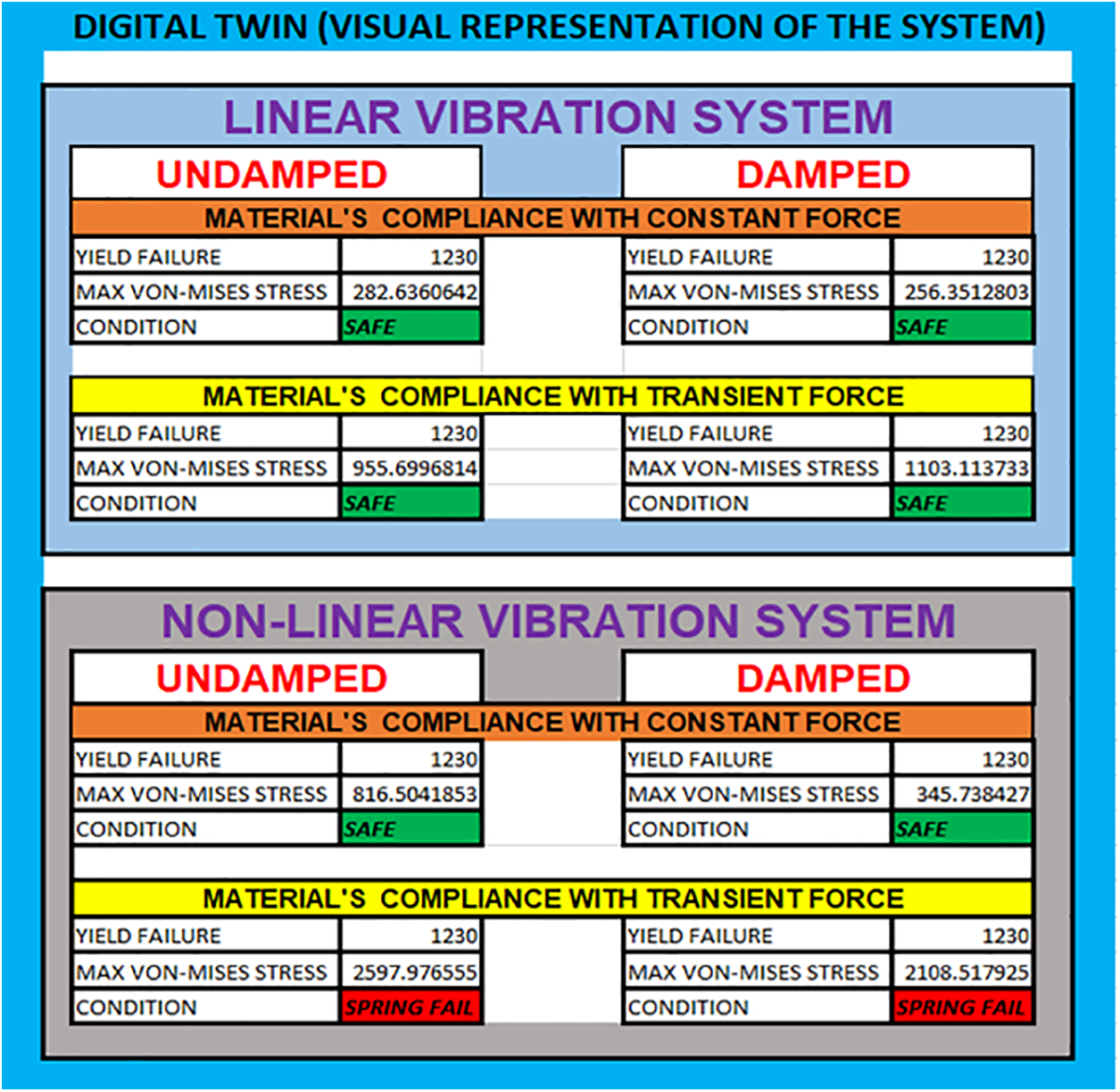
Figure 11: A sample of the DT model used in this research

5  Conclusion

This paper proposed a novel numerical concept of the Digital Twin based on Euler’s method. The Digital Twin model successfully replicated the mechanical behaviour and virtually represented the mechanics of materials for the physical coiled spring. Successfully developed a numerical way to validate the proposed idea of the DT. The technique suggested still has limitations and is subject to further research. This paper defined the Digital Twin as “Digital Twin is a virtual replica of anything, where the replication must mirror the entire internal and external mechanical behaviour of the replicated thing.”. The DT model virtually represented all stresses acted internally on the spring. While the resulting strains and stresses are accurate based on Euler’s method, this paper proposed a novel concept for the DT. The DT model captured all the variations of the normal and maximum induced shear stress in current real-time. Additionally, the model showed the instant representation of the system’s behaviour and showed that in the case of free force, vibration behaved similarly concerning the time is irregular compared to the conduct of the linear-steady forced vibration system. The damping effect into the system mentioned in the section of the undamped linear transient-forced vibration system leads the output response slightly distorted compared to the rest of the spring’s motion within the first few seconds of the spring’s motion’s movement observed.

The non-linear steady and transient forced vibration used in the un-damped case illustrates all measurements’ output response (deflection, strain, maximum normal and induced shear stresses). The output for each of the four springs behaves harmonically with the same natural frequency, with different values concerning the time due to the other geometric properties of each spring. Non-Linear Steady-Forced Vibration Systems (Damped) is the same as the undamped system. The only difference is throughout the analysis of springs’ motions within the system, which is attached to the base neither gets extended nor extended gets compressed. The model shows the overall displacement of the coils and the displacement between each coil. The model still has some limitations and is open for further research; fatigue analysis is one of most types of failure accrues to mechanical systems. Since all the stresses shown in the model’s interface are in the current real-time, it is essential to improve the fatigue analysis further.

Acknowledgement: The authors would like to thank the Society of Automotive Engineers (SAE), for making the data available on their website.

Funding Statement: The authors did not receive funding for this research study.

Author Contributions: The authors of this research paper have made equal contributions to the study from inception to completion. Each author has played a significant role in conceiving and designing the research, collecting and analysing data, interpreting results, and writing and revising the manuscript. Specifically, each author has collaboratively formulated the research objectives and hypotheses, participated equally in data collection, either through experiments, surveys, or data acquisition, conducted statistical analyses and interpreted the findings jointly, contributed equally to the drafting and revision of the manuscript, including the literature review and discussion sections, and reviewed and approved the final version of the manuscript for submission. We affirm that all authors have made substantial and equal contributions to this research and are in full agreement with the content of the manuscript.

Availability of Data and Materials: The data and materials supporting the findings of this study are available at https://www.sae.org/. We are committed to promoting transparency and facilitating further scientific inquiry, and we will make every effort to provide the necessary information and resources to interested parties in a timely manner.

Conflicts of Interest: The authors declare that they have no conflicts of interest to report regarding the present study.

References

1. Qi, Q., Tao, F. (2018). Digital twin and big data towards smart manufacturing and industry 4.0: 360 degree comparison. IEEE Access, 6, 3585–3593. [Google Scholar]

2. Wang, L., Törngren, M., Onori, M. (2015). Current status and advancement of cyber-physical systems in manufacturing. Journal of Manufacturing Systems, 37, 517–527. [Google Scholar]

3. Ross, D. (2016). Digital twinning. Engineering and Technology, 11, 44–45. [Google Scholar]

4. He, B., Bai, K. J. (2021). Digital twin-based sustainable intelligent manufacturing: A review. Advances in Manufacturing, 9, 1–21. [Google Scholar]

5. Boschert, S., Rosen, R. (2016). Digital twin—the simulation aspect, mechatronic futures, pp. 59–74. Switzerland: Springer International Publishing. [Google Scholar]

6. Gupta, B. B., Tewari, A. (2020). A beginner’s guide to Internet of Things security: Attacks, applications, authentication, and fundamentals. USA: CRC Press. [Google Scholar]

7. Boje, C., Guerriero, A., Kubicki, S. et al. (2020). Towards a semantic construction digital twin: Directions for future research. Automation in Construction, 114, 103179. [Google Scholar]

8. O’donovan, P., Leahy, K., Bruton, K. et al. (2015). An industrial big data pipeline for data-driven analytics maintenance applications in large-scale smart manufacturing facilities. Journal of Big Data, 2015, 2–26. [Google Scholar]

9. Lee, J., Azamfar, M., Singh, J. (2019). A blockchain enabled cyber-physical system architecture for industry 4.0 manufacturing systems. Manufacturing Letters, 20, 34–39. [Google Scholar]

10. Wang, J., Ye, L., Gao, R. X. et al. (2019). Digital twin for rotating machinery fault diagnosis in smart manufacturing. International Journal of Production Research, 57, 3920–3934. [Google Scholar]

11. Moor, J., Minsky, M., Shannon, C. (2006). Artificial intelligence conference: The next fifty years. AI Magazine, 27, 87–91. [Google Scholar]

12. Glaessgen, E. H., Stargel, D. S. (2019). The digital twin paradigm for future NASA and U.S. air force vehicles. 53rd Structures, Structural Dynamics, and Materials Conference, Honolulu, Hawaii, USA. [Google Scholar]

13. Lim, K. Y. H., Zheng, P., Chen, C. H. (2020). A state-of-the-art survey of Digital Twin: Techniques, engineering product lifecycle management and business innovation perspectives. Journal of Intelligent Manufacturing, 31, 1313–1337. [Google Scholar]

14. Ríos, J., Hernández, J. C., Oliva, M., Mas, F. (2015). Product avatar as digital counterpart of a physical individual product: Literature review and implications in an aircraft. Advances in Transdisciplinary Engineering, 2, 657–666. [Google Scholar]

15. Vom Brocke, J., Simons, A., Niehaves, B. et al. (2009). Reconstructing The giant: On the importance of rigour in documenting the literature search process. The 17th European Conference on Information Systems (ECIS), Verona, Italy. [Google Scholar]

16. Lee, J., Lapira, E., Bagheri, B. et al. (2013). Recent advances and trends in predictive manufacturing systems in big data environment. Manufacturing Letters, 1(1), 38–41. [Google Scholar]

17. Weber, C., Königsberger, J., Kassner, L. et al. (2017). M2DDM—A maturity model for data-driven manufacturing. Procedia CIRP, 63, 173–178. [Google Scholar]

18. Zhuang, C., Liu, J., Xiong, H. (2018). Digital twin-based smart production management and control framework for the complex product assembly shop-floor. The International Journal of Advanced Manufacturing Technology, 96, 1149–1163. [Google Scholar]

19. Fukawa, N., Rindfleisch, A. (2023). Enhancing innovation via the digital twin. International Journal of Production Research, 2022, 320–325. [Google Scholar]

20. Zheng, P., Lin, T. J., Chen, C. H. et al. (2018). A systematic design approach for service innovation of smart product-service systems. Journal of ProdcutInovation Management, 201, 657–667. [Google Scholar]

21. Antonova, E. E., Looman, D. C. (2005). Finite elements for thermoelectric device analysis in ANSYS. 24th International Conference on Thermoelectrics, pp. 215–218. Clemson, USA. [Google Scholar]

22. Reinhart, C., Breton, P. F. (2009). Experimental validation of autodesk® 3ds Max® design. The Journal of the Illuminating Engineering Society, 6, 7–35. [Google Scholar]

23. Merhi Bleik, J., Alhamzawi, B. (2019). Fully Bayesian estimation of simultaneous regression quantiles under asymmetric laplace distribution specification. Journal of Probability and Statistics, 2019, 8610723. [Google Scholar]

24. Rosenblum, J. P. (2016). An overview of flow control activities at dassault aviation over the last 25 years. The Aeronautical Journal, 120, 391–414. [Google Scholar]

25. Dixon, S., Irshad, H., Pankratz, D. M. et al. (2019). The 2019 deloitte city mobility index. gauging global readiness for the future of mobility. Deloitte Insights, 18, 2–14. [Google Scholar]

26. Lohr, B. S. (2016). G.E., the 124-year-old software start-up. The New York Times, 34, 1–8. [Google Scholar]

27. Garud, R., Kumaraswamy, A., Sambamurthy, V. (2006). Emergent by design: Performance and transformation at Infosys technologies. Organization Science, 17(2), 277–286. [Google Scholar]

28. Jain, S. K., Marceau, G., Zhang, X., Koved, L. (2006). INTELLECT: INTErmediate-language LEvel C translator. Computer Science, 123, 60–67. [Google Scholar]

29. Sequeira, A. A., Singh, R. K., Shetti, G. K. (2016). Comparative analysis of helical steel springs with composite springs using finite element method. Journal of Mechanical Engineering and Automation, 6, 63–70. [Google Scholar]

30. Lee, J., Azamfar, M., Singh, J. et al. (2020). Integration of digital twin and deep learning in cyber-physical systems: Towards smart manufacturing. IET Collaborative Intelligent Manufacturing, 2, 34–36. [Google Scholar]

31. Lee, C. G., Park, S. C. (2014). Survey on the virtual commissioning of manufacturing systems. Journal of Computational Design and Engineering, 1, 213–222. [Google Scholar]

32. Muzaffar, S., Elfadel, I. M. (2020). Shoe-integrated, force sensor design for continuous body weight monitoring. Sensors, 20(12), 1–22. [Google Scholar]

33. Reddy, R., Sujith, L. N. (2017). A comprehensive literature review on data analytics in IIoT (Industrial Internet of Things). IEEE Access, 8, 2757–2764. [Google Scholar]

34. Jeong, K., Choi, S. (2019). Model-based sensor fault diagnosis of vehicle suspensions with a support vector machine. International Journal of Automotive Technology, 20, 961–970. [Google Scholar]

35. Brandyberry, M. D., Tuegel, E. J., Gockel, B. T. et al. (2012). Challenges with structural life forecasting using realistic mission profiles. Structural Dynamics and Materials Conference, Honolulu, Hawaii, USA. [Google Scholar]

36. Zhuang, C., Liu, J., Xiong, H. (2018). Digital twin-based smart production management and control framework for the complex product assembly shop-floor. International Journal of Advanced Manufacturing Technology, 96, 1149–1163. [Google Scholar]

37. Gupta, K., Shukla, S. (2016). Internet of Things: Security challenges for next generation networks. 2016 1st International Conference on Innovation and Challenges in Cyber Security, pp. 315–318. Greater Noida, India. [Google Scholar]

38. Zhang, H., Liu, Q., Chen, X., Zhang, D., Leng, J. (2017). A digital twin-based approach for designing and multi-objective optimization of hollow glass production line. IEEE Access, 5, 26901–26911. [Google Scholar]

39. Tao, F., Cheng, J., Qi, Q., Zhang, M., Zhang, H. et al. (2018). Digital twin-driven product design, manufacturing and service with big data. International Journal of Advanced Manufacturing Technology., 94, 3563–3576. [Google Scholar]