Fault Ride-Through (FRT) Behavior in VSC-HVDC as Key Enabler of Transmission Systems Using SCADA Viewer Software

1  Introduction

The development of interconnected national and international power grid networks has necessitated relatively long transmission lines. Stability issues in three-phase power transmission systems are caused by the different voltage angles. Furthermore, depending on the load, a line generates or consumes reactive power. Furthermore, it was demonstrated that the voltage source converter (VSC)-based high voltage direct current (HVDC) system has some limitations [1]. Cable routes without elaborate compensation facilities are approximately 80.0 km long due to their high mutual capacitance. The charging current has a continuous cable current at this critical length without transmitting active power to the consumer [1,2].

A line also produces or consumes reactive or active power depending on whether the load on the line is low or high. Due to their high mutual capacitance, cable routes without elaborate compensation facilities can only be established up to the length of a transmission line. Early on, attempts were made to use high direct current (DC) voltages for power transmission [3–5]. One challenge for voltage source converter (VSC)-based VSC-HVDC transmission systems is the fault ride through (FRT) capability specified by grid codes [3,6]. The FRT capability allows VSC-HVDC transmission systems to continue operating normally in the presence of abnormal alternating current conditions such as voltage deviations [7,8]. Zero voltage ride-through (ZVRT), low voltage ride-through (LVRT), and high voltage ride-through (HVRT) are all FRT specifications (HVRT).

The FRT has piqued the interest of many scientists, with the majority of them focusing on methods for improving the FRT capability of wind turbines connected to an AC grid via a VSC-HVDC transmission system [6,9]. The authors of [9] proposed a new control strategy for ensuring wind fault ride-through in their paper [9]. Using nonlinear adaptive VSC-HVDC control, the approach in [10] could improve wind farm FRT capability. To reduce post-fault disturbances, the control method could temporarily disable the converters and take appropriate actions. The overcurrent was limited, the wind turbines remained operational, and the alternating current voltage quickly recovered [11–13]. The research work cited in [14] proposes a strategy for recovering from DC faults. A high rating series diode valve was installed at each VSC inverter pole to reduce fault currents. The researchers in [15,16] proposed FRT control and management schemes for the VSC-HVDC system.

The converter control strategy in VSC-HVDC is critical for improving its FRT capability [17–22]. The work done in [17] proposed a strategy for reducing the inverter side-overvoltage of the HVDC system in the event of an inverter side Ac system fault. The authors in [18] presented a new static synchronous compensator operating model for the recently published alternative arm converter. The concept in [19] proposed a new FRT method that did not rely on direct data exchange between two double star chopper (DSCC) converters. The authors of [20] developed a perturbation observer-based sliding-mode control scheme to control VSC-HVDC systems. The authors of [21] proposed a passive control scheme for multi-terminal VSC-HVDC systems to provide reliable and effective integration of electrical power from renewable energy. The authors of [22] proposed the negative sequence controller needed for such asymmetrical conditions in AC grids.

The authors of [21] proposed a passive control method for multi-terminal VSC-HVDC systems to provide efficient and consistent integration of electrical power from renewable energy. The authors of [22] proposed the negative sequence controller needed for such asymmetrical conditions in AC grids. The passive control scheme was proposed in [21] for multi-terminal VSC-HVDC systems to provide reliable and effective integration of renewable energy. In [22], the authors proposed the negative sequence controller that is required for such asymmetrical conditions in AC grids.

2  The Power Flow in the Occurrence of Fault-Based HVDC Systems

The primary goal of power flow in the event of a fault is to investigate the effect of faults on power transfers through various sequences, as well as to analyze the role of power flow direction and voltage sag magnitude, as shown in Fig. 3. The Figs. 1a and 1b depict the steady-state condition and the utility grid side fault, respectively [17].

Figure 1: The position of Us,˙Uc˙, and the direct axis and quadrature axis

The most severe fault condition in HVDC transmission systems is a pole-to-pole short-circuit fault. It generates high currents in HVDC systems and damages converter devices in a short period of time. Furthermore, in HVDC transmission line systems, pole-to-ground faults do not pass extremely high currents through the converters [17,18]. The analysis shows that when a network experiences severe faults, the active and reactive power transfer between stations 1 and 2 decreases. As shown in Fig. 1 [19], the voltage in the direct and quadrature axis’s component are changed.

3  Fault Analysis in Symmetrical Components Based on HVDC Systems

The majority of traveling waves produced by faults in HVDC circuits are computed and compared using disparate analytical methods. For efficient design protection, there is a lot of research being done on fault characteristics in bipolar HVDC lines. Traveling waves are unsymmetrical due to fault location in multi-terminal HVDC systems, but symmetrical component analysis is used for fault detection in HVDC systems [21].

3.1 The Equations for Symmetrical Components

The voltage ua and ub and current vectors ia and ib determine their components using zero and positive sequence [22]. But, the negative sequence components are not readily determined using balanced load conditions and may heighten phase-to-phase faults.

{ua=ua0+ua1ub=ub0+ub1,{ub0=ua0ub1=ua1(1)

The general equations to determine the sequence quantities for positive, negative, and zero sequence components from a three-phase system, as [23–26]

{u0=13(ua+ub+uc)u1=13(ua+aub+a2uc)u2=13(ua+a2ub+auc)(2)

{i0=13(ia+ib+i)i1=13(ia+aib+a2ic)i2=13(ia+a2ib+aic)(3)

where {a=1∠1200a2=1∠2400 and a is a mathematical identity, u0, i0 are zero sequence voltage and current, u1, i1 are positive sequence voltage and current, and u2,i2 are negative sequence voltage and current.

3.2 Mathematical Modeling of Power Flow within Stations

The powers (active power and reactive power) exchange between stations 1 and 2 must have boundaries based on mathematical equations of power transfer. However, the purpose of calculating active power and reactive exchanged between stations make the capability curve of stations to be recognized and identify if is station 1, or station 2 is injecting, or absorbing power based on mathematical equations written in [20]. If it is assumed that the transmission lines have small resistance compared to the reactance and R = 0.0 (Z = X < 90°). Consequently, the mathematical equations are

P=UsUrsin⁡δXL(4)

Q=Us(Us−Urcos⁡δ)XL(5)

Squaring both Eqs. (4) and (5) based on different assumptions, separating, and factorizing all terms containing sine and cosine, we get the following equations:

(P)2=(UsUrXLsin⁡δ)2(6)

From Eq. (5), some terms can be put together as follows:

Q=UsUs−UsUrcos⁡δXL⇒Q=Us2XL−UsUrcos⁡δXL

and provides Eq. (7)

(Q−Us2XL)2=(−UsUrcos⁡δXL)2(7)

Therefore, the addition of Eqs. (6) and (7) and factorizing active power and reactive power as follows:

P2+(Q−Us2XL)2=(UsUrXL)2(cos2⁡δ+sin2⁡δ)⇒P2+(Q−Us2XL)2=(UsUrXL)2(8)

Recall that cos2⁡δ+sin2⁡δ=1 as a trigonometric rule then Eq. (8) becomes

P2+(Q−Us2XL)2=(UsUrXL)2(9)

Let us assume that Q=0.0 so that Eq. (9) gives Eq. (10):

P2+(Us2XL)2=(UsUrXL)2(10)

Then the active power is calculated as shown in Eq. (11):

⇒P=(UsUrXL)2−(Us2XL)2(11)

From Eq. (11), the range of active power (P) exchanged between stations 1 and 2, is confined to the following range:

−(UsUrXL)2−(Us2XL)2≤P≤(UsUrXL)2−(Us2XL)2(12)

The reactive power in VAR (Q) exchanged between stations 1 and 2 is obtained from Eq. (9) as follows:

(Q−Us2XL)2=(UsUrXL)2−P2 and taking the square root of both sides of Eq. (9) becomes

⇒(Q−Us2XL)2=(UsUrXL)2−P2⇒(Q−Us2XL)=(UsUrXL)2−P2 then

Q=(UsUrXL)2−P2+Us2XL(13)

So, from Eq. (13), the range of reactive power in VAR (Q) is as follows:

−(UsUrXL)2−P2+Us2XL≤Q≤(UsUrXL)2−P2+Us2XL(14)

where Us is sending end voltage, Ur is receiving end voltage, XL is line impedance between buses, and δ is the angle between sending end and receiving end voltage.

3.3 Fault Location Techniques in HVDC Transmission

For optimal power system operation, fault localization and identification have become critical. Furthermore, many methods have demonstrated limitations such as automation, fault clearing time, and outage time. Multi-terminal HVDC (MT-HVDC) grids lack the ability to control power flow in a self-sufficient manner [27]. Impedance-based techniques, traveling wave techniques [28,29], machine learning techniques, and Time Domain Reflection (TDR) techniques [24–27] are the four (4) fault location methods.

In transmission line propagation, transient disturbances generate traveling waves, which involve voltages and currents. Since 1950, the method of traveling waves has been used to estimate fault location. It is used on a small scale, but it is accurate and efficient [21,25–27]. The recognition and selection of surges and fault-induced transients measured at line terminals is required for the current HVDC system fault location of traveling waves. These also have an impact on the accuracy of fault location. When the transmission consists of more than two segments, it is difficult to identify traveling waves. This is due to the requirement for high-frequency sampling in high-velocity wave propagation.

The mathematical morphology (MM) [29] method has a set of filters that can extract specific signal characteristics by leveraging its geometry [28–30]. Natural frequency extraction (NFE) [28] is a distributed parameter model that is used for fault localization and identification. Laplace transforms [31,32] are used to calculate the wave speed and boundary conditions. The empirical mode decomposition (EMD) [28] and wavelet packet decomposition (WPD) [28] methods produce an overall complete feature of signals for interpretation by generalizing multiresolution analyses and entire families of sub-band decomposition elements [33,34].

Fast-forward control is used in artificial intelligence techniques based on radial basis function neural networks (RBF-NNs), which have three layers: an input layer, a hidden layer, and an output layer [34,35]. Using weighted connections and node activation functions, RBF-NNs use the human neuron concept to complete the machine learning and pattern recognition processes. On the transmission line, the EMTR-based fault location relies solely on the time-reversal invariance of the telegraph equations [36]. The Fourier transform of a function f(t) that integrates a real and symmetric window at frequency w is the short time-frequency transforms (STFT) (t) [37]. Time is used to translate it, and frequency is used to modulate it. The STFT is a quantitative analysis of high-frequency components in the occurrence of fault currents [38]. However, the paper [38,39] included a table comparing the benefits and drawbacks of frequency domain and time domain.

3.4 Type of Fault in High Voltage Transmission Line and HVDC

There is different type of fault in an HVDC system like AC faults, DC faults and internal converter. The faults are normally provoked by the failure of short circuits, switching and lightning events and mostly associated by insulation [40]. In an HVDC system, there are three types of faults: AC faults, DC faults, and internal converter faults. Faults are typically caused by the failure of short circuits, switching, and lightning events, and are frequently associated with insulation [40].

3.4.1 Type of DC Faults

The following are the DC faults: DC line-to-line, DC line-to-ground, and DC double line-to-ground faults [40,41]. A line-to-line fault is a very dangerous type of DC fault that occurs during the operation of a VSC-HVDC system and consists of three stages: capacitor discharge, grid current feeding phases, and diode freewheeling. DC line-to-ground faults are common and are primarily dependent on the grounding system of the HVDC system. The responses of the DC voltage and current under double line-to-ground faults are referred to as DC double line-to-ground faults. Following the fault event, there are three stages: capacitor discharging (Stage 1), diode freewheeling (Stage 2), and grid current feeding (Stage 3).

3.4.2 Timing Diagram for HVDC System

The HVDC system’s protection strategy is based on primary and backup safeguards. At the ends of transmission lines, protective devices such as relays and circuit breakers (CBs) are installed and react accordingly [41]. Figs. 2a and 2b show the timing diagram for an HVDC system and positive sequence in α,β, and dq synchronous reference frame for a HVDC system protection: t0 is the time when the DC fault in the network occurs and the primary relay begins sensing the fault. At time t1, the primary protection relay sends a tripping signal to the associated circuit breaker, and at time t2, the circuit breaker immediately responds to the trip signal by opening its contacts devices to interrupt the dc fault current. Typically, the backup relay detects the fault at time t2, and a backup trip signal is generated at time t3.

Figure 2: Timing diagram and positive sequence in α,β, and dq synchronous reference frame for a HVDC system protection

If primary protection fails completely to interrupt the current in the interval between t2 and t4, backup breaker initiates its process of interruption at time t4. The fault is completely interrupted and cleared by backup protection in the interval between t2 and t5 [41].

3.4.3 The Research Gaps

•   AC transmission over long distances has revealed some challenges, such as technical and commercial losses as a result of insufficient testing. However, in HVDC transmission, some stations may behave as sending or receiving systems depending on the power settings, and if a fault occurs in the network, it may easily lose synchronism and some signals are greatly affected while others are not.

•   Furthermore, some VSC-HVDC networks have revealed some challenges, such as poor performance of proportional integrals (PIs) or proportional integral derivative (PIDs).

3.5 The Main Contribution of this Research are Listed as Follows

•   To develop a practical method for testing the fault ride through capability of VSC-HVDC transmission system based on the platform in a high E-Tech smart grid laboratory of the ACE-ESD.

•   To give an extensive experimental verification of the proportional-integral PI) control performance for voltage and current loops.

•   To analyze the effectiveness and competitiveness of DC chopper for voltage stabilization and excess energy management.

3.6 The Reactive Current Support in the Event of a Fault of HVDC Technology

Under utility grid faults, utility grid operators provide fast reactive current injection, which activates protective relays and utility grid voltage support [42]. As a result, reactive current injection from wind farms based on the doubly-fed induction generator (DFIG) is no longer required by transmission system operators on a national and international scale. As a result, many European countries have reached an agreement on grid code requirements for dynamic grid fault tolerance and under-voltage ride-through conditions. Furthermore, for positive sequence, the reactive current injection is at least 2.0 percent of the rated current for every percent of voltage sag and reaches 90.0 percent of the steady-state value in 50.0 ms [43].

Referring to Fig. 2b, the AC currents in the dqo synchronous reference frame are shown

ddt[idiq]=[−RLω−ω−RL][idiq]+1L[usd−ucdusq−ucq](15)

The active and reactive power in balanced mode [42]:

{Pac=VdId+VqIqQac=VdIq−VqId(16)

And the power on the DC side is calculated as follows:

Pdc=idc.udc+cducdt.uc=(VdId+VqIq)(17)

Eqs. (16) and (17) represent the VSC-HVDC equations under asymmetric conditions. As shown in Figs. 3–5, the positive sequence (pos) space vector rotates counterclockwise, whereas the conjugate complex negative sequence (neg) space vector rotates in the opposite direction. The space vectors of positive and negative sequences (neg) voltage in the, and reference frames are aligned to the corresponding phase angles represented in the synchronously rotating reference frame in these figures.

Figure 3: The negative sequence in α,β, and dq in the synchronous reference frame [44]

Figure 4: Diagram of the current loop

Figure 5: Current loop based on positive and negative sequence with PI controllers

Some assumptions were made for unbalanced VSC-HVDC systems, and zero sequence components do not exist. Under asymmetric conditions, three-phase voltages and currents decouple into positive (pos) and negative (neg) components [45]. As shown in Eqs. (18) and (19) [44,45], the above factors result in a separation of voltages and currents into direct and quadrature axes dqo synchronous reference frame:

(ucdpucqp)=Lddt(idpiqp)+(−RωL−ωL−R)(idpiqp)+(usdpusqp)(18)

(ucdnucqn)=Lddt(idniqn)+(−RωL−ωL−R)(idniqn)+(usdnusqn)(19)

where the subscripts “p” and “n” symbolize positive and negative components, respectively. Therefore, active power and reactive power inputs at the point of common coupling (PCC) are as follows [45]:

S=UsDQ.IDQ~˙=(ejωtusdqp+e−jωtusdqn)(ejωtidqp+e−jωtidqn)(20)

{p(t)=p0+pc2cos⁡(2ωt)+ps2sin⁡(2ωt)q(t)=q0+qc2cos⁡(2ωt)+qs2sin⁡(2ωt)(21)

where p0 and q0 are averages of active power and reactive power separately, pc2 and ps2 are cosine and sinusoidal 2nd harmonic peak active power (P), and qc2, qs2 are cosine and sinusoidal 2nd harmonic peak reactive power (Q). The power-balance equation for the DC side of the unbalanced condition becomes

Pdc=idc.udc+cducdt.uc=p(t)(22)

4  HVDC Technologies

4.1 Mathematical Modeling of Voltage and Current Loops

Naturally, the switching operation from the rectifier to the inverter has many challenges like harmonics and voltage fluctuations, which are resolved using either first or second-order filters. Thus, root locus, bode diagram, or mathematical equations are not entirely sufficient because an inverter should be controlled [44,45].

Determination of Voltage and Current Loop Equations

Eq. (23) determines the current loop based on proportional integral and derivate (PID), and proportional-plus-integral (PI) controllers, with filters and dqo [45]:

{ucd*=−(kp+kiS)(id*−id)−ωLiq+usducq*=−(kp+kiS)(iq*−iq)+ωLid+usq(23)

where ucd*, ucq∗ are the reference voltages used to control VSC. The tracking voltages rely on the reference voltages in the voltage loop. Also, kp and ki are proportional and integral gains of the inner loop controller, which increase the tracking signals up to the reference voltages, and remove the harmonics. id∗,id, iq*,iq are reference currents in the current loop stabilized by proportional-integral (PI) controllers from the Eq. (18). The HVDC systems represented in Fig. 3 have the advantage of being simulated either as 300.0 km or 150.0 km and advantage is that a sensor is installed inside an obstacle the powers supply is adjustable to any desired voltage level [41].

The VSC-HVDC has some drawbacks. It is sensitive to utility grid disturbances. When faults occur, negative-sequence (neg) components exist in the utility grid. The voltage converter performance will be poor because of harmonics and other unwanted signals that lead to losses. Because positive-sequence currents are always higher than the negative-sequence currents in the grid, new equations control the positive-sequence (pos) currents. However, negative-sequence (neg) components are a disturbance. The control loop equations consider only positive-sequence (pos) components and the voltage loop equations become [39]

{ucdp*=−(kp+kiS)(idp*−idp)−ωLiqp+usdpucqp*=−(kp+kiS)(iqp*−iqp)+ωLidp+usqp(24)

And the equations during disturbance for negative sequence voltage loops are [45]

{ucdp*=−(kp+kiS)(idp*−idp)−ωLiqp+usdp+usdnucqp*=−(kp+kiS)(iqp*−iqp)+ωLidp+usqp+usdn(25)

where ucdp*, and ucqp* are reference voltages in the positive synchronous reference frame, while ucq*, and ucd* are voltages in positive sequence components. The negative sequence is controlled and stabilized by PI controllers. The usdn are negative sequence utility grid source voltages in the positive synchronous reference frame. Also, iqp*,idp* are positive currents in a synchronous reference frame in which the feed-forward is decoupled and controlled [39] as summarize mathematically in Eqs. (31) and (32).

4.2 Control Strategies and Protection Techniques Used in This Work

DC chopper device was used to control and stabilize dc link voltage, DC relay for protection of current, and time over/undervoltage relay was used as well. The synchronization device which was able to track if the condition of synchronization are satisfied before connecting the stations and line side controller for controlling and stabilize the transmission line parameters which were the sending voltage, active power and reactive power. Besdides, that the dynamic grid fault simulator device with SCADA VIEWER were used as well for creating and clearing a fault in network while SCADA VIEWER software was used to supervise, control and data acquisition of the network. Additionally, the SCADA VIEWER was able to track the following errors overvoltage and undervoltage for DC link, phase sequence for grid, phase grid, grid undervoltage and overvoltage, grid fault, line side controller overcurrent and undercurrent.

5  Experimental Setup of VSC-HVDC System Based on SCADA Viewer Software

5.1 Description of the Experimental Setup

Fig. 6 is an experimental setup consisting of a converter station, which transforms the conventional electricity grid alternating voltage into direct voltage through a 300.0 km transmission line. A second converter station at the other end converts the direct voltage back into an alternating voltage. Energy was transmitted in both directions. HVDC converter station 1 regulated voltage and converter station 2 regulated the power. Additionally, the experimental setup has a DC chopper to stabilize DC voltage, dissipate energy in case of a fault, and autonomous control of reactive power, active power, frequency, and voltage using the supervisory control and data acquisition (SCADA) Viewer software package.

Figure 6: Experimental hardware test bed with SCADA Viewer software

Additionally, Fig. 6 is the dynamic grid fault simulator that mimics the voltage sag in three-phase networks. It is feasible to study the response of devices connected downstream (mains connection, control elements, liquid crystal display (LCD), pre-selection disruption L1, L2, and L3, test object connection). Table 1 is the dataset of each device used in the experiments. Evaluation of different fault conditions in the network conform to the voltage sag values of the dynamic grid simulator. Also, there was power transfer from one station to the other.

The experimental results are carried out through different scenarios and listed as follows:

•   Power flow in the event of a fault,

•   Reactive current support in the event of a fault,

•   The mains voltage in asymmetric faults via SCADA Viewer software and dynamic grid fault simulator.

Scenario 1: Power flow in the event of a fault in the HVDC system

Table 2 shows the dataset for the power flow in the event of a fault. The influence of faults on the active and reactive power transfer capabilities was evaluated. It also considers both the power flow direction and the voltage dip magnitude. The power transfer was 80.0% of the rated power for station 1 (rectifier). Similarly, the voltage sag was 60.0% of the rated voltage. Thus, the rectifier in station 1 absorbed active power from the inverter in station 2 (Table 2).

Fig. 7 comprise input values of UL−L=400.0V at AC source (station 1), 80.0%  rated power transfer, 60.0%  rated voltage (voltage sag), 0.0 in phase-quadrature coefficient (IQ), and 0.0 dead band of the positive sequence. During the fault, the voltage fluctuations in station 2 depend on the fault type. But, the voltage in station 1 remains approximately constant during the fault ride-through (FRT), as in Fig. 7.

Figure 7: A positive sequence of the mains voltage Ugrid in station 1 (rectifier)

Fig. 8 has essentially the same input parameters as Fig. 7. During a fault, the quadrature axis current remains at roughly the same level (±0.125p.u.) throughout the fault period. But, the direct axis component current lies between −0.656and+0.125p.u. during the fault and the transmitted power decreases. The quadrature axis current fluctuated with the harmonics that originated from the conversion of AC to DC (rectifier). It remained negative when the switching frequency was between 12.0 and 20.0 kHz, respectively (as shown by the pulse width modulation (PWM) clock in Fig. 9.

Figure 8: A positive sequence of the current Igrid in station 1 (rectifier)

Figure 9: A positive sequence of the current Igrid in station 2 (inverter)

Fig. 9 shows that when a fault occurs in the network, the current in station 2 (inverter) remains roughly at the same level as if outside of the fault period, while the voltage at the inverter side sags depending on fault type. The current in station 1 (rectifier) reduces drastically during the fault leading to a decrease in transmitted power. The direct axis current (Id) slightly fluctuated while the quadrature axis current (Iq) remained relatively constant during the fault.

Fig. 10 used the data of Table 2 to indicate the direct axis voltage (Vd) when a fault occurred in the network at 0.2 s. The voltage decreased when the fault occurred from 0.2 to 0.4 s and was then cleared by the SCADA Viewer. Meanwhile, the voltage at the quadrature axis (Vq) was not affected during the disturbance from 0.2 up to 0.4 s. The power (Pdc=−691.0W) was negative at station 1 (rectifier), and on the other side, the power on the DC side at station 2 was positive (Pdc=733.0W) because it worked as an inverter. Also, around 80.0% of the rated power was transferred from station 2 to station 1 (as indicated by the arrow and the values recorded in Table 2). The inverter control triggered switching operations between the voltage and current loops based on the 15.0 kHz PWM clock frequency.

Figure 10: The positive sequence of the mains voltage Ugrid at station 2 (inverter)

Fig. 11 shows that both the DC voltage (Udc) and DC current (Idc) remain approximately constant, outside the fault region. The DC current dips during the fault, which leads to the drop in the power flow during the fault condition. However, the voltage at the rectifier side was approximately constant during a fault ride-through (FRT) and stayed synchronized using the capability of FRT with the SCADA Viewer.

Figure 11: Voltage and current on the DC side

Fig. 12 shows that the voltages at the utility grid in the direct and quadrature axes were slightly affected during a fault. It was only at 0.2 s when a fault occurred that the voltage ripple appeared. The fault was cleared and then reoccurred at 0.4 s. The negative sequence voltage remained constant as indicated by Fig. 13 at 0.10 dead-band.

Figure 12: The voltage at the utility grid side for a negative sequence (Ugrid)

Figure 13: The current at the utility grid side for zero sequences (Igrid)

Fig. 13 indicates that the current at the utility grid was constant for a zero sequence when a fault occurs in the network and later cleared by the SCADA Viewer. The inverter switching operations triggered at 15.0 kHz and the voltage dip was 60.0% of the rated voltage for the line-to-line fault. The ripple effect decreased during the fault occurring between 0.2 and 0.4 s.

Fig. 14 shows that the currents of the utility grid in the direct and quadrature axes were not affected during the fault. But only in the negative sequence component that experienced the fault in the network. The fault was cleared using the SCADA Viewer and the dynamic grid fault simulator. The negative sequence voltage remained relatively constant at 0.10 dead-band. Station 2 parameters comprise the following: Vl12=399.0V, Vl23=399.0V, Vl31=402.0V, and 60.0% rated voltage as voltage dip. The active power was adjusted to 80.0% of the rated power. Also, station 1 had the following data: Vl12=411.0V, Vl23=411.0V, Vl31=412.0V, and 60.0% rated voltage as voltage dip.

Figure 14: The current at the utility grid side of the negative sequence (Igrid)

Fig. 15 showed that the voltage at the utility grid side was constant for a zero sequence when a fault occurred in the network. The fault was cleared by the SCADA Viewer software package. The switching operations triggered the inverter using 15.0 kHz. The line-to-line fault voltage dip was 60.0% of the rated voltage. For 2000.0 ms time duration, the inverter supplying station 1 behaved as a rectifier.

Figure 15: The voltage at the utility grid side for zero sequences (Ugrid)

Fig. 16 showes the signals obtained based on the data in Table 2. The voltage at the direct current side fluctuated during the fault, whatever the variations of IQ and dead band. Also, the DC current (Idc) fluctuated between 0.2 and 0.4 s, during a fault in the network. The instantaneous voltage (Ugrid) also suffered fluctuations during the fault condition as shown in Fig. 16. There was system restoration after the fault was cleared by the SCADA Viewer and dynamic grid simulator. Furthermore, the instantaneous current (Igrid) decreased, and reached −1.1 p.u. (the negative side), because of a fault.

Figure 16: The instantaneous voltage and current for the utility grid and their DC values

Generally, these cases showed that the DC voltage remains approximately constant and the DC current dipped during the fault.

Scenario 2: Reactive current support in the event of a fault

This section investigates the impact of reactive current support in the event of a fault. The active power transferred 80.0% of the rated power while the voltage sag was 60.0% of the rated voltage. Furthermore, the reactive current determines the influence of IQ on POS gain. Consequently, the dataset of Table 3 as input for the reactive current support in the event of a fault using the SCADA Viewer.

The active power was 80.0% of the rated power transfer while the voltage sag was 60.0% of the rated voltage. Fig. 17 indicates that the inverter was not synchronized to the grid. The steady-state error (SSE) between the inverter and utility grid was little, compared to the IEEE 1547 standards. The SSEs occurring between the angular speed and voltage of the inverter and the utility grid were similar. The controller adjustments reduced the SSEs between the reference and tracking signals. Also, the voltage and current loops combined with the proportional-integral (PI) control stabilized the network. Furthermore, the output signals (dqo) fed the PWM with 15.0 kHz for switching operations.

Figure 17: Unsynchronized to the utility grid

Fig. 18 showed that after controlling the voltage loop and current loop based on the filter values, the inverter was synchronized to the utility grid. That means that the steady-state error between frequency, voltage, angular speed, and the phase sequence was relatively small.

Figure 18: Synchronized to the utility grid

Fig. 19 contains the input values of UL−L=400.0V at the AC source (terminal 1). Eighty percent of the rated power (power transfer), sixty percent of the rated voltage (voltage sag), in phase-quadrature coefficient (IQ), and zero dead band were the parameters of the negative sequence. Although various gain settings did not affect quadrature voltage (Vq), larger gains increased the direct voltage (Vd) component in the event of a fault.

Figure 19: The voltage at the utility grid station of station 2 with positive sequence

Fig. 20 shows the currents at the utility grid side for both the direct and quadrature axes components comprising 0.10 dead-band and 0.0 IQ, respectively. The direct axis current (Id) slightly fluctuated during faults in the network, around 0.2 s and between 0.4 and 0.5 s. Furthermore, the quadrature current (Iq) also fluctuated in synchronism with, but slightly lower than Id. After the faults were cleared by the SCADA Viewer and the dynamic grid fault simulator, the currents returned to their initial values.

Figure 20: The positive sequence of the current Igrid at station 2 with 0.0 gain

Fig. 21 shows that the in-phase quadrature coefficient (IQ) increased between −0.1 p.u. and +0.4 p.u., for a fault occurring between 0.20 and 0.40 s. The direct axis component of the positive sequence fluctuated slightly before and after the fault.

Figure 21: The positive sequence of the current Igrid at station 2 with a gain of 0.5

Fig. 22 indicates that the IQ coefficient increased from −0.1 p.u. to +0.6 p.u. (between 0.2 and 0.4 s), and decreased from +0.6 to 0.0 p.u. (between 0.4 and 0.5 s), respectively. Also, the direct axis component ranged between +0.7 p.u. and +1.0 p.u. during the fault (from 0.2 to 0.5 s duration). Both the direct axis and quadrature axis components returned to their steady-state values after the fault.

Figure 22: The positive sequence of the current Igrid at station 2 with 1.0 gain

Fig. 23 shows that the IQ coefficient increased from 0.0 to +0.8 p.u. when a fault occurred between 0.20 and 0.40 s. Both the direct axis and quadrature axis components returned to their initial values after the fault. That means that IQ has a substantial impact on quadrature axis voltage or current during the transient disturbance. Although there were harmonics, the SCADA Viewer and dynamic grid simulator were effective and competent at clearing the fault.

Figure 23: A positive sequence of the current Igrid at station 2 with an IQ = 1.5, gain

Fig. 24 shows that an increase in the IQ coefficient made the quadrature axis component of the positive sequence increase when a fault occurred between 0.20 and 0.40 s (−0.1 to +1.1 p.u.). Also, it subsequently returned to the initial value after the fault. Furthermore, the direct axis current (Id) component fluctuated moderately and remained essentially stable after the fault.

Figure 24: A positive sequence of the current Igrid at station 2 with an IQ = 2.0, gain

Fig. 25 indicates an increase in the IQ coefficient made the quadrature axis component of the positive sequence change when a fault occurs between 0.20 and 0.40 s (−0.1 to +1.1 p.u.). Also, the current in the direct axis component was faintly affected and remained substantially at the initial level.

Figure 25: The positive sequence of the current Igrid at station 2 has a 2.5, gain

Fig. 26 indicates a rise in the IQ coefficient. The quadrature axis component of the positive sequence increased during the fault and returned to the initial value after the fault. Furthermore, the direct axis component was imperceptibly affected but remained basically at the initial level. That means that IQ has a substantial impact on the quadrature axis voltage or current during the transient disturbance. Although some harmonics were present in the network, both the SCADA Viewer software and the dynamic grid simulator cleared the fault.

Figure 26: A positive sequence of the current Igrid at station 2 has a 3.0, gain

Fig. 27 shows an increase in the IQ coefficient, which made the quadrature axis component of the positive sequence increase. The fault occurred between 0.20 and 0.40 s and between 0.4 and 0.5 s, respectively, before returning to the initial state after the fault. The quadrature axis component voltage was unaffected by any fault and remained stable in the network. That means that IQ has a substantial impact on quadrature axis voltage or current during the transient disturbance. The experimental results showed that the voltage at the utility grid of the quadrature axis was unaffected and remained at the initial value. The various gain settings did not significantly affect the current Id (+0.7 and +1.1 p.u.), and large gains increased the current Iq in the event of a fault, and the current Iq ranged between −0.1 and 1.1p.u., respectively. The direct axis voltage (Vd), hovered around +0.35 and +1.10 p.u., respectively. Additionally, the transient fault effects occurred between 0.2 and 0.5 s for both the Vd and Iq, respectively. Consequently, the response remains unchanged at higher gain values, and the current character is independent of the power flow.

Figure 27: Ugrid and Igrid at station 2 when IQ = 3.0 and dead band 0.1

Scenario 3: The mains voltage in the case of asymmetric faults

Table 4 shows the dataset for the mains voltage in the scenario of asymmetric faults using the SCADA Viewer software and dynamic grid fault simulator to determine the mains voltage in the event of a 2-pole fault without earth contact, and also determine the mains voltage in the event of a 1-pole fault. Therefore, the main objective is to analyse the influence of power transfer, IQ value, and voltage sag in the HVDC system. Consequently, the power transfer was 80.0% of the rated power, IQ equals 1.0, while the voltage sag was 100.0% of the rated voltage (as shown in Table 4).

Fig. 28 shows the effect of a fault in the network on the instantaneous voltage for the utility grid side. But, the presence of the SCADA Viewer software and dynamic grid fault simulator cleared the fault. The voltage returned to its steady-state value, even in the presence of harmonics. During a fault, the voltage decreased to zero. Fig. 29 shows the positive sequence status of the main voltage Ugrid at station 2 with a dead band = 0.1.

Figure 28: Instantaneous values of the mains voltage Ugrid at the inverter side

Figure 29: A positive sequence of the mains voltage Ugrid at station 2 with a dead band = 0.1

Fig. 29 shows that the direct axis voltage component decreased in the network within the time interval 0.2 and 0.4 s. The instantaneous voltage at the quadrature axis was constant before, during, and post fault in the network.

Fig. 30 indicated that the voltage in the quadrature and direct axes remained in their initial positions after the fault. Only the voltage at the direct axis experienced some transients during and after the fault occurred from 0.20 to 0.40 s. But it returned to its initial level after the fault.

Figure 30: A negative sequence of the mains voltage Ugrid in station 2

Fig. 31 shows that at zero sequences, the voltage at dqo did not change during a fault in the network, and the signal remained at its initial state.

Figure 31: Zero sequences of the voltage Ugrid at station 2

Fig. 32 shows that the direct current voltage (Udc) changed slightly when a fault occurred in the network and remained stable within the stability margin. The direct current (Idc) significantly changed during a fault in the network at the time interval of 0.2 and 0.4 s. The direct axis current decreased during a fault in the network and slowly increased with some harmonics until reaching the stability region. Meanwhile, the quadrature current was unchanged during the fault in the network and both the dead band and IQ were constant.

Figure 32: Udc, Idc, and Id, Iq at the positive sequence

Fig. 33 shows that the direct current voltage (Udc) lightly changed when a fault occurred in the network and remained within the stability region even though the direct current (Idc) had changed when a fault occurred in the network at the time interval of between 0.2 and 0.4 s.

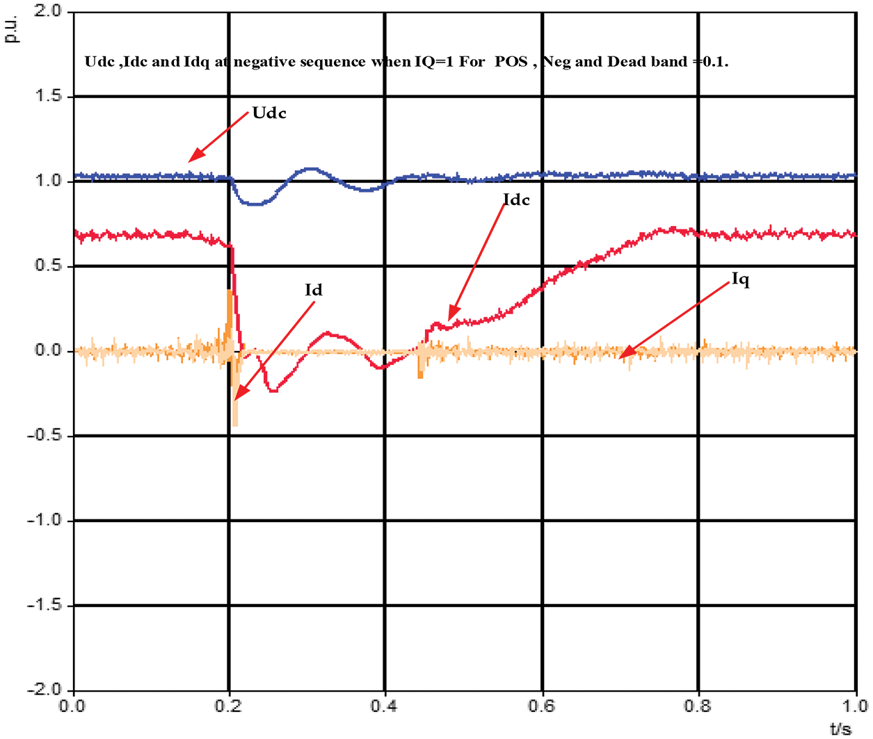
Figure 33: Udc, Idc and Idq at negative sequence with IQ = 1.0 and dead band = 0.10

The direct axis current fluctuated during a fault in the network and slowly increased with some harmonics until reaching the stability region. Furthermore, the quadrature current was relatively unchanged during the fault even though with 0.1 dead-band and 1.0 IQ, respectively.

Fig. 34 shows that the direct current voltage (Udc) slightly changed when a fault occurred in the network and remains at the stability margin. However, the direct current (Idc) significantly changed when a fault occurred between 0.2 and 0.4 s. The direct axis current changed notably during the fault and slowly increased with harmonics until reaching the stability region. Error-prone phases break down during the fault, which mutually overlaps, and are displaced by 180° with each other.

Figure 34: Udc,Idq, and Idc at zero-sequence with IQ = 1.0 for pos

Fig. 35 shows that the direct current voltage (Udc) was changed when a fault occurred in the network and stayed within the stability margin even though the direct current (Idc) remarkably changed and reached a negative value during the fault in the time interval between 0.2 and 0.4 s. The direct axis current also outstandingly changed during the fault and gradually increased with harmonics until reaching the stability region. Furthermore, the quadrature current did not change during the fault even though the dead band was 0.10 and IQ was kept at 1.50.

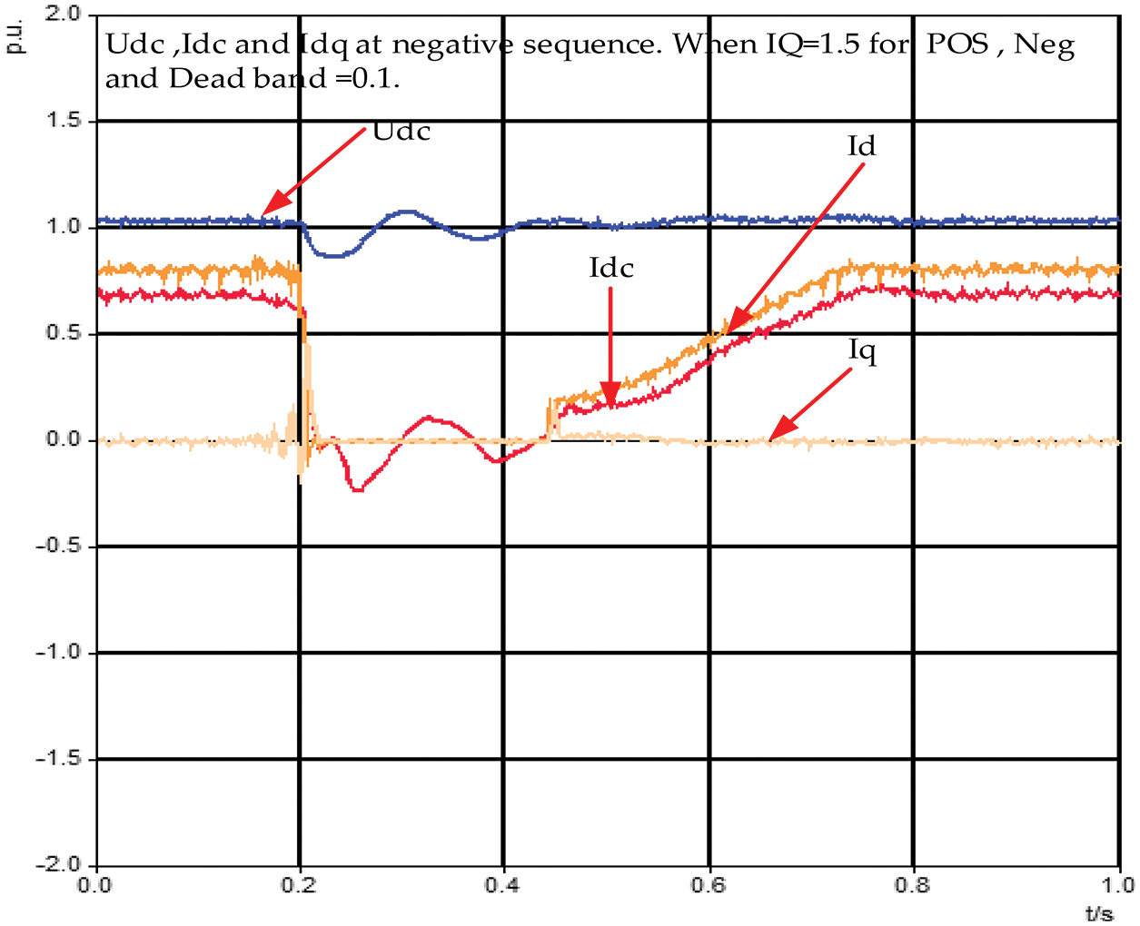
Figure 35: Udc,Idq and Idc at positive sequence with IQ = 1.5

Fig. 36 indicates that the direct current voltage (Udc) slightly changed when a fault occurred in the network and remained within the stability margin even though the direct current (Idc) crucially changed and reached a negative value in the time interval between 0.2 and 0.4 s. The direct axis current also significantly changed during the fault and steadily increased with harmonics until it reached the stability region. Also, the quadrature current was unchanged during the fault, and the dead band was 0.10, and IQ was 2.0. Moreover, both the direct and quadrature axes currents for zero-sequence did not experience any change or faults when faults occurred in the network.

Figure 36: Udc, Idc, and Idq for the positive sequence with IQ = 2.0

Fig. 37 indicates that the direct current voltage did not change during the fault in the network. Also, the direct current remained the same because it did not experience any fault. Furthermore, both the direct and quadrature axes currents were remarkably changed, during the fault in conjunction with harmonics.

Figure 37: Udc and Idc with Q = 50% and IQ = 2.0, then dead-band = 0.1

Fig. 38 showes the impact of fault on the network and on the direct axis voltage, which changed to zero during a fault occurring between 0.2 and 0.4 s. After the fault was cleared, the voltage returned to the nominal value. Also, the quadrature axis voltage remained in the zero references at IQ = 3.0 for the positive sequence.

Figure 38: The positive sequence of the mains voltage Ugrid at station 2, and IQ = 3.0

Fig. 39 shows the impact of fault on the direct axis voltage in the network. Significant changes occurred until the parameters became zero during the fault in the network (between 0.2 and 0.4 s). After the fault, the voltage returned to the nominal value (Ud), but the quadrature axis voltage (Uq) remained at the zero references when IQ = 3.0, and 0.1 dead bands for the positive sequence. But, the direct axis current (Id) decreased rapidly between 0.2 and 0.4 s before returning to its nominal state. Furthermore, both the voltage and current at the quadrature axis did not change.

Figure 39: A positive sequence of the mains voltage Ugrid at station 2

Fig. 40 shows that the direct current voltage fluctuated sharply when a fault occurred in the network. The DC current (Idc) was substantially changed and reached a negative value, but the SCADA Viewer restored it to the nominal range. Although the SCADA Viewer and the dynamic grid fault simulator restored Udc, Igrid, the instantaneous current shows very many harmonics and fluctuations before, and after a fault in the network.

Figure 40: Udc, Idc, Igrid instantaneous when IQ = 3.0 and dead band = 0.1

6  Conclusion

The VSC-HVDC systems FRT behavior was investigated using the High-E Tech smart grid laboratory of the African Centre of Excellence in Energy for Sustainable Development (ACE-ESD), University of Rwanda, as in Fig. 8. The results show that fault ride-through with SCADA Viewer software and dynamic grid fault simulator is more adaptable and suitable for HVDC transmission line faults. The study can be harmonized to satisfy the connection requirements for HVDC paths worldwide, especially for regions requiring long transmission lines.

Additionally, fault ride-through capability, dynamic voltage regulations, and associated rise times for HVDC systems could be used to set standards because IQ largely affects the quadrature axis voltage and current components. The experimental results reveal that the negative sequence current opposes the negative sequence voltage by lowering the power output. A negative quadrature current (Iq) of the negative sequence is inductive and a positive quadrature current (Iq) of the positive sequence is capacitive.

During experiments, the SCADA Viewer software and dynamic grid fault simulator showed that the stations (rectifier or inverter) either inject or absorb active power or reactive power from each other. At 100.0% rated power, station 1 absorbs −775.0 W active power, and generates 164.0 W at 0.0% power transfer rate. At −100.0% rated power, the rectifier injected 1264.0 W into the network. The IQ amplitude and quadrature axis component assessment show that the quadrature axis current increase depends upon the IQ in faults. It can also impact current loop control. The system offers numerous possibilities for a more detailed treatment of specific aspects and examination of other parameters that overcome losses in HVDC transmission lines.

Future research can be recommended to will be focus on:

Applicability, controllability, affordability, and accessibility of HVDC technologies in East African Community Countries because some countries are lagging behind in meeting the targets of 2030 in complying with the Paris Agreement.

Impact of high integration of distributed energy resources (DERs) with electric vehicles and electric motorcycles because EVs generate instability and different types of harmonics in the network.

Control strategies of HVDC using the traditional droop control are normally modified and there are more than 15 types of modified droop control systems.

Funding Statement: Authors are grateful to Quanzhou Tongjiang Scholar Special Fund for financial support through Grant No. (600005-Z17X0234); Quanzhou Science and Technology Bureau for financial support through Grant No. (2018Z010), and Huaqiao University through Grant No. (17BS201); and the Fujian Provincial Department of Science and Technology for financial support through Grant (2018J05121). Authors are also grateful for financial support from the Fujian Provincial Department of Science and Technology through Grant Nos. (2021I0014) and (2018J05121).

Conflicts of Interest: The authors declare that they have no conflicts of interest to report regarding the present study.

References

 1.  Hu, J., He, Z., Lin, L., Xu, K., Qiu, Y. (2018). Voltage polarity reversing-based DC short circuit FRT strategy for symmetrical bipolar FBSM-MMC HVDC system. IEEE Journal of Emerging and Selected Topics in Power Electronics, 6(3), 1008–1020. DOI 10.1109/JESTPE.2018.2820076. [Google Scholar] [CrossRef]

 2.  van der Meer, A. A., Ndreko, M., Gibescu, M., van der Meijden, M. A. (2015). The effect of FRT behavior of VSC-HVDC-connected offshore wind power plants on AC/DC system dynamics. IEEE Transactions on Power Delivery, 31(2), 878–887. DOI 10.1109/TPWRD.2015.2442512. [Google Scholar] [CrossRef]

 3.  Flourentzou, N., Agelidis, V. G., Demetriades, G. D. (2009). VSC-based HVDC power transmission systems: An overview. IEEE Transactions on Power Electronics, 24(3), 592–602. DOI 10.1109/TPEL.2008.2008441. [Google Scholar] [CrossRef]

 4.  Dambone Sessa, S., Chiarelli, A., Benato, R. (2019). Availability analysis of HVDC-VSC systems: A review. Energies, 12(14), 2703. DOI 10.3390/en12142703. [Google Scholar] [CrossRef]

 5.  Alassi, A., Bañales, S., Ellabban, O., Adam, G., MacIver, C. (2019). Transmissão HVDC: Revisão de tecnologia, tendências de mercado e perspectivas futuras. Renewable and Sustainable Energy Reviews, 112(1), 530–554. DOI 10.1016/j.rser.2019.04.062. [Google Scholar] [CrossRef]

 6.  Patil, P. R., Bhole, A. A. (2017). A review on enhancing fault ride-through capability of distributed generation in a microgrid. IEEE 2017 Innovations in Power and Advanced Computing Technologies (i-PACT), pp. 1–6. Vellore, India: IEEE. [Google Scholar]

 7.  Yaramasu, V., Wu, B., Sen, P. C., Kouro, S., Narimani, M. (2015). High-power wind energy conversion systems: State-of-the-art and emerging technologies. Proceedings of the IEEE, 103(5), 740–788. DOI 10.1109/JPROC.2014.2378692. [Google Scholar] [CrossRef]

 8.  Feltes, C., Wrede, H., Koch, F. W., Erlich, I. (2009). Enhanced fault ride-through method for wind farms connected to the grid through VSC-based HVDC transmission. IEEE Transactions on Power Systems, 24(3), 1537–1546. DOI 10.1109/TPWRS.2009.2023264. [Google Scholar] [CrossRef]

 9.  Sang, Y., Yang, B., Shu, H., An, N., Zeng, F. et al. (2019). Fault ride-through capability enhancement of type-4 WECS in offshore wind farm via nonlinear adaptive control of VSC-HVDC. Processes, 7(8), 540. DOI 10.3390/pr7080540. [Google Scholar] [CrossRef]

10. Vrionis, T. D., Koutiva, X. I., Vovos, N. A., Giannakopoulos, G. B. (2007). Control of an HVDC link connecting a wind farm to the grid for fault ride-through enhancement. IEEE Transactions on Power Systems, 22(4), 2039–2047. DOI 10.1109/TPWRS.2007.907377. [Google Scholar] [CrossRef]

11. Ramtharan, G., Arulampalam, A., Ekanayake, J. B., Hughes, F. M., Jenkins, N. (2009). Fault ride through of fully rated converter wind turbines with AC and DC transmission systems. IET Renewable Power Generation, 3(4), 426–438. DOI 10.1049/iet-rpg.2008.0018. [Google Scholar] [CrossRef]

12. Sun, W., Torres-Olguin, R. E., Anaya-Lara, O. (2016). Investigation on fault-ride through methods for VSC-HVDC connected offshore wind farms. Energy Procedia, 94(1), 29–36. DOI 10.1016/j.egypro.2016.09.185. [Google Scholar] [CrossRef]

13. Haleem, N. M., Rajapakse, A. D., Gole, A. M., Fernando, I. T. (2018). Investigation of fault ride-through capability of hybrid VSC-LCC multi-terminal HVDC transmission systems. IEEE Transactions on Power Delivery, 34(1), 241–250. DOI 10.1109/TPWRD.2018.2868467. [Google Scholar] [CrossRef]

14. Li, Y., Liu, C., Tian, X., Wang, Z. (2019). Study on fault ride-through control of islanded wind farm connected to VSC-HVDC grid based on the VSC converter AC-side bus forced short circuit. The Journal of Engineering, 16(16), 3325–3328. DOI 10.1049/joe.2018.8421. [Google Scholar] [CrossRef]

15. Moawwad, A., El Moursi, M. S., Xiao, W. (2016). Advanced fault ride-through management scheme for VSC-HVDC connecting offshore wind farms. IEEE Transactions on Power Systems, 31(6), 4923–4934. DOI 10.1109/TPWRS.2016.2535389. [Google Scholar] [CrossRef]

16. Zhou, Z., Chen, Z., Wang, X., Du, D., Yang, G. et al. (2019). AC fault ride through control strategy on inverter side of hybrid HVDC transmission systems. Journal of Modern Power Systems and Clean Energy, 7(5), 1129–1141. DOI 10.1007/s40565-019-0546-1. [Google Scholar] [CrossRef]

17. Feldman, R., Farr, E., Watson, A. J., Clare, J. C., Wheeler, P. W. et al. (2014). DC fault ride-through capability and STATCOM operation of a HVDC hybrid voltage source converter. IET Generation, Transmission & Distribution, 8(1), 114–120. DOI 10.1049/iet-gtd.2012.0713. [Google Scholar] [CrossRef]

18. Oguma, K., Akagi, H. (2017). Low-voltage-ride-through performance of an HVDC transmission system using two modular multilevel double-star chopper-cells converters. Electrical Engineering in Japan, 200(1), 33–44. DOI 10.1002/eej.22976. [Google Scholar] [CrossRef]

19. Yang, B., Sang, Y. Y., Shi, K., Yao, W., Jiang, L. et al. (2016). Design and real-time implementation of perturbation observer-based sliding-mode control for VSC-HVDC systems. Control Engineering Practice, 56(4), 13–26. DOI 10.1016/j.conengprac.2016.07.013. [Google Scholar] [CrossRef]

20. Yang, B., Jiang, L., Yu, T., Shu, H. C., Zhang, C. K. et al. (2018). Passive control design for multi-terminal VSC-HVDC systems via energy shaping. International Journal of Electrical Power & Energy Systems, 98(3), 496–508. DOI 10.1016/j.ijepes.2017.12.028. [Google Scholar] [CrossRef]

21. Dumnic, B., Popadic, B., Milicevic, D., Vukajlovic, N., Delimar, M. (2019). Control strategy for a grid connected converter in active unbalanced distribution systems. Energies, 12(7), 1362. DOI 10.3390/en12071362. [Google Scholar] [CrossRef]

22. Latorre, H. F., Ghandhari, M., Söder, L. (2008). Active and reactive power control of a VSC-HVdc. Electric Power Systems Research, 78(10), 1756–1763. DOI 10.1016/j.epsr.2008.03.003. [Google Scholar] [CrossRef]

23. Nelson, J. P., Panetta, S. (2019). High resistance grounding analysis using symmetrical components. 2019 IEEE PES/IAS PowerAfrica, pp. 445–451. Abuja, Nigeria, IEEE. [Google Scholar]

24. He, L., Hao, L., Qiao, W. (2019). Remote monitoring and diagnostics of pitch bearing defects in a MW-scale wind turbine using pitch symmetrical-component analysis. 2019 IEEE Energy Conversion Congress and Exposition (ECCE), pp. 1–6. Baltimore, MD, USA, IEEE. [Google Scholar]

25. Rouzbehi, K., Yazdi, S. S. H., Moghadam, N. S. (2018). Power flow control in multi-terminal HVDC grids using a serial-parallel DC power flow controller. IEEE Access, 6, 56934–56944. DOI 10.1109/ACCESS.2018.2870943. [Google Scholar] [CrossRef]

26. Muzzammel, R. (2019). Restricted Boltzmann machines-based fault estimation in multi terminal HVDC transmission system. International Conference on Intelligent Technologies and Applications, pp. 772–790. Singapore, Springer. [Google Scholar]

27. Zhang, S., Zou, G., Huang, Q., Gao, H. (2018). A traveling-wave-based fault location scheme for MMC-based multi-terminal DC grids. Energies, 11(2), 401. DOI 10.3390/en11020401. [Google Scholar] [CrossRef]

28. Mangalge, S. M., Jawale, S. D. (2016). A review on fault location techniques in Long HVDC transmission lines. International Journal of Advanced Research in Electrical, Electronics and Instrumentation Engineering, 5(5), 4220–4226. DOI 10.15662/IJAREEIE.2016.0505064. [Google Scholar] [CrossRef]

29. Tzelepis, D., Psaras, V., Tsotsopoulou, E., Mirsaeidi, S., Dyśko, A. et al. (2020). Voltage and current measuring technologies for high voltage direct current supergrids: A technology review identifying the options for protection, fault location and automation applications. IEEE Access, 8, 203398–203428. DOI 10.1109/ACCESS.2020.3035905. [Google Scholar] [CrossRef]

30. Jia, H. (2017). An improved traveling-wave-based fault location method with compensating the dispersion effect of the traveling wave in the wavelet domain. Mathematical Problems in Engineering, 2017(8), 1–11. DOI 10.1155/2017/1019591. [Google Scholar] [CrossRef]

31. Triveno, J. P., Dardengo, V. P., de Almeida, M. C. (2015). An approach to fault location in HVDC lines using mathematical morphology. 2015 IEEE Power & Energy Society General Meeting, pp. 1–5. Denver, CO, USA, IEEE. [Google Scholar]

32. Muo, U. E., Madamedon, M., Ball, A. D., Gu, F. (2017). Wavelet packet analysis and empirical mode decomposition for the fault diagnosis of reciprocating compressors. 2017 23rd International Conference on Automation and Computing (ICAC), pp. 1–6. Huddersfield, UK, IEEE. [Google Scholar]

33. Shah, S., Hassan, R., Sun, J. (2013). HVDC transmission system architectures and control-A review. In the 2013 IEEE 14th Workshop on Control and Modeling for Power Electronics (COMPEL), pp. 1–8. Salt Lake City, UT, USA, IEEE. [Google Scholar]

34. Jia, J., Yang, G., Nielsen, A. H. (2017). A review on grid-connected converter control for short-circuit power provision under grid unbalanced faults. IEEE Transactions on Power Delivery, 33(2), 649–661. DOI 10.1109/TPWRD.2017.2682164. [Google Scholar] [CrossRef]

35. Shabestary, M. M., Mohamed, Y. A. R. I. (2018). Asymmetrical ride-through and grid support in converter-interfaced DG units under unbalanced conditions. IEEE Transactions on Industrial Electronics, 66(2), 1130–1141. DOI 10.1109/TIE.2018.2835371. [Google Scholar] [CrossRef]

36. Zhang, J., Chen, R., Xiao, L. S., Guo, X. C., Liu, B. (2017). Optimal control for AC and DC power quality of VSC-HVDC. 2017 International Conference on Computer Systems, Electronics and Control (ICCSEC), pp. 1649–1658. Dalian, China, IEEE. [Google Scholar]

37. Jackson, R., Zulkifli, S. A., Sham, N. M. B., Pathan, E. (2019). An investigation on active and reactive power flow control based on grid-tied parallel inverters. AIP Conference Proceedings, 2173(1), 020001. DOI 10.1063/1.5133916. [Google Scholar] [CrossRef]

38. Wijnhoven, T., Deconinck, G., Neumann, T., Erlich, I. (2014). Control aspects of the dynamic negative sequence current injection of type 4 wind turbines. 2014 IEEE PES General Meeting| Conference & Exposition, pp. 1–5. National Harbor, MD, USA, IEEE. [Google Scholar]

39. Camacho, A., Castilla, M., Miret, J., de Vicuña, L. G., Guzman, R. (2017). Positive and negative sequence control strategies to maximize the voltage support in resistive-inductive grids during grid faults. IEEE Transactions on Power Electronics, 33(6), 5362–5373. DOI 10.1109/TPEL.2017.2732452. [Google Scholar] [CrossRef]

40. Yin, Z., Qiu, H., Yang, Y., Tang, Y., Wang, H. (2020). Practical submodule capacitor sizing for modular multilevel converter considering grid faults. Applied Sciences, 10(10), 3550. DOI 10.3390/app10103550. [Google Scholar] [CrossRef]

41. Liu, Y., Huang, M., Qu, L., Zha, X. (2017). Interaction of voltage and current control loop in three-phase voltage source converter. IECON 2017-43rd Annual Conference of the IEEE Industrial Electronics Society, pp. 6847–6852. Beijing, China, IEEE. [Google Scholar]

42. Nduwamungu, A. (2017). Review on the coordination and energy management of microgrids broad-based on PQ controller and droop control. Some useful information is given in this paper. Open Access Library Journal, 4(7), 1–8. DOI 10.4236/oalib.1103719. [Google Scholar] [CrossRef]

43. Nduwamungu, A. (2018). Energy management and control strategy of DC source and microturbine generation system by using PQ controller and droop control in islanded mode. International Journal of Energy and Power Engineering, 7(1), 9. DOI 10.11648/j.ijepe.s.2018070101.12. [Google Scholar] [CrossRef]

44. Qin, J., Saeedifard, M., Rockhill, A., Zhou, R. (2014). The hybrid design of modular multilevel converters for HVDC systems based on various submodule circuits. IEEE Transactions on Power Delivery, 30(1), 385–394. DOI 10.1109/TPWRD.2014.2351794. [Google Scholar] [CrossRef]

45. Nami, A., Liang, J., Dijkhuizen, F., Demetriades, G. D. (2014). Modular multilevel converters for HVDC applications: Review on converter cells and functionalities. IEEE Transactions on Power Electronics, 30(1), 18–36. DOI 10.1109/TPEL.2014.2327641. [Google Scholar] [CrossRef]