Optimization of Blade Geometry of Savonius Hydrokinetic Turbine Based on Genetic Algorithm

Nomenclature

1  Introduction

In recent years, with the increase of the world’s population, countries around the world are facing different degrees of energy crisis. As a result, countries began to switch from fossil energy to renewable energy, hydropower is a kind of power generation technology that can alleviate the pressure of fossil energy demand to a certain extent [1–3]. Large hydropower stations need to utilize the potential energy generated by the water level difference between upstream and downstream to generate electricity. People have different reviews of such behavior. The small hydropower station appeared, with a preference for gaining energy directly from low-velocity water [4,5]. Savonius hydrokinetic turbine is a kind of turbine which works under the condition of small velocity. Under the condition that velocity is greater than 0.5 m/s, the Savonius turbine can work well and produce certain efficiency, this kind of turbine is suitable for hydropower generation and transmission in remote areas and poor geographical environments [6–8].

The Savonius turbine is characterized by its ability to work harmoniously at low velocity without causing significant damage to fish populations and the work environment [9,10]. The early Savonius turbine was designed with an S-blade runner, which has stable working performance but low working efficiency, and some people have studied the blade shape optimization of the Savonius turbine. The work characteristics of the Savonius turbine are analyzed under steady inlet velocity conditions, and the effects of blade overlap ratio, clearance ratio, blade chord length, blade number and tip speed ratio on turbine performance are figured out. Thiyagaraj et al. [11] studied how to improve the power coefficient of the Savonius turbine by changing the number of blades, overlap ratio and increasing overturning. The power coefficients under different blade numbers and overlap ratios are analyzed. Bian et al. [12] analyzed the flow field performances of the Savonius turbine based on CFD and explored the influence of tip speed ratio and overlap ratio on the power coefficient. Kumar et al. [13] concentrated on the study of the Savonius turbine runner. Compared with the two-blade and three-blade runner, the four-blade Savonius runner performance is worse. Mosbahi et al. [14] studied how to improve the efficiency of the Savonius runner by changing the blade shape, and used CFD to simulate the different blade shapes, and optimized the power coefficient according to the tip speed ratio and the blade shape. Hashem et al. [15] took a pair of swimming koi carp as inspiration and carried out a CFD-based optimization design for the Savonius turbine, mainly aiming at the blade overlap ratio and clearance ratio to enhance the power coefficient on the meta-model. Wang et al. [16] optimized the design of the Savonius wind turbine with a double-sided contour, using sliding network technology to build CFD models, and optimized the double-sided shape of the runner based on the Kriging-PSO optimization model. Finally, the turbine performance was significantly improved. Shashikumar et al. [17] studied the performance of conventional and tapered turbine blades in hydroelectric power generation was investigated and it was found that the loss of energy measured at the outlet of the advancing blade of the tapered turbine resulted in a 5% reduction in performance. Additionally, Shashikumar et al. [18] also studied the Savonius turbine with different tip speed ratios using the dynamic grid technique and showed that the maximum torque coefficient and power coefficient for tip speed ratios of 0.22 and 0.17 were 0.7 and 0.9. Khani et al. [19] first used different software calculation methods such as Catboost, artificial neural networks, and random forests to predict the power coefficients of the Savonius hydrodynamic turbine, and the results showed that the Catboost method was more accurate. Wu et al. [20] combined the fast Fourier transform and dynamic modal decomposition to provide an in-depth analysis of the frequency distribution and dynamic patterns of velocity fluctuations in the near wake region, comparing the advantages and disadvantages of the two methods and providing a new approach to flow analysis.

It is found that the blade geometry is the key to the power coefficient performance of the Savonius turbine. When evaluating the performance of the Savonius turbine, the value of the maximum power coefficient and the value of the high-power coefficient range should also be considered. This is a typical bi-objective optimization study [21,22]. Using an algorithm to optimize design is a method often used in engineering work. It is not only widely used in water turbines, but also widely used in air turbines, pumps and so on. Based on the genetic algorithm, Chan et al. [23] optimized the blade shape of the Savonius wind turbine with conventional semi-circular blades to further improve the power coefficient. Jia et al. [24] optimized the Savonius wind turbine blade shape based on a support vector regression agent model and an improved flower pollination algorithm. The optimized wind turbine has a better ability to catch wind than the conventional semicircular blade turbine. Mohamad et al. [25] optimized the design of centrifugal pumps based on the Particle swarm optimization, optimizing the shape of the centrifugal pump runner to increase efficiency and head. Oyama et al. [26] optimized the design of a rocket engine pump based on an evolutionary algorithm, using the concept of a single-stage centrifugal pump to enhance the design. After optimization, the total head of the unit is superior to the original design, and the input power is reduced by 1%. Wu et al. [27] used the discrete particle swarm optimization algorithm to optimize the array of tidal turbines, by redefining the particle velocity to optimize the position of each tidal turbine. Based on the genetic algorithm, Han et al. [28] optimized the design of wind turbine blades by using induced iterative initialization. Lu et al. [29] optimized the design of the rotor blade and guide vane shape of the OWC device based on a genetic algorithm and artificial neural network, and the results showed that the energy loss of the optimal blade shape was greatly reduced and there was a significant widening of the efficient range of the OWC device.

In the process of optimization design, the flow characteristics in the runner blade region and the energy loss at the blade can be analyzed by means of computational fluid dynamics (CFD). Based on the entropy production theory, Chang et al. [30] analyzed the energy loss of the self-priming pump, and analyzed the type, magnitude and location of hydraulic loss under different blade thickness distributions. Su et al. [31] analyzed the performance and energy loss of the high-speed centrifugal pump with straight blades, combined with the flow stability analysis, and introduced the entropy production method to evaluate the mechanical loss. Ghorani et al. [32] utilized the theory of entropy production, and a pump was used as a turbine in the numerical study of the mechanism of energy dissipation. In this paper, entropy production theory and the second law of thermodynamics are used to study the problem of energy loss inside the pump. Based on entropy production, Wang et al. [33] optimized the geometric parameters of the pump as the impeller of a steam turbine under three different typical flow conditions. An entropy production rate analysis can effectively explain the energy loss phenomenon.

The main research object of this paper is the Savonius turbine with an S-shaped blade, in which the geometric shape of the runner blade is the key point of the optimization design. The optimization will consider dual performance parameters as the objective function, and the genetic algorithm will be utilized as the foundational technique for achieving this objective. The relationship between the blade overlap ratio, clearance ratio, blade circumferential angle and the maximum power coefficient and high-power coefficient range of the Savonius turbine will be deeply analyzed and expounded. The influence of runner blade geometry on turbine performance will be thoroughly studied, which will provide technical support for hydropower generation in conditions of small flow velocity.

2  Model and Parameters Profiles of Savonius Turbine

Fig. 1 below shows a two-dimensional model of the Savonius turbine, serving as the key point of this paper. As the computational domain of the Savonius turbine is very wide compared to the runner computational domain and the results near the edges do not affect the runner computational domain, we saved both computational resources and time costs by reducing the three-dimensional model to two dimensions [34,35]. The turbine is composed of four key components: inlet, outlet, interface and runner blade. At low velocity, water flows from the inlet through the runner and blade, producing torque under the combined action of the two blades, and then flows out of the outlet.

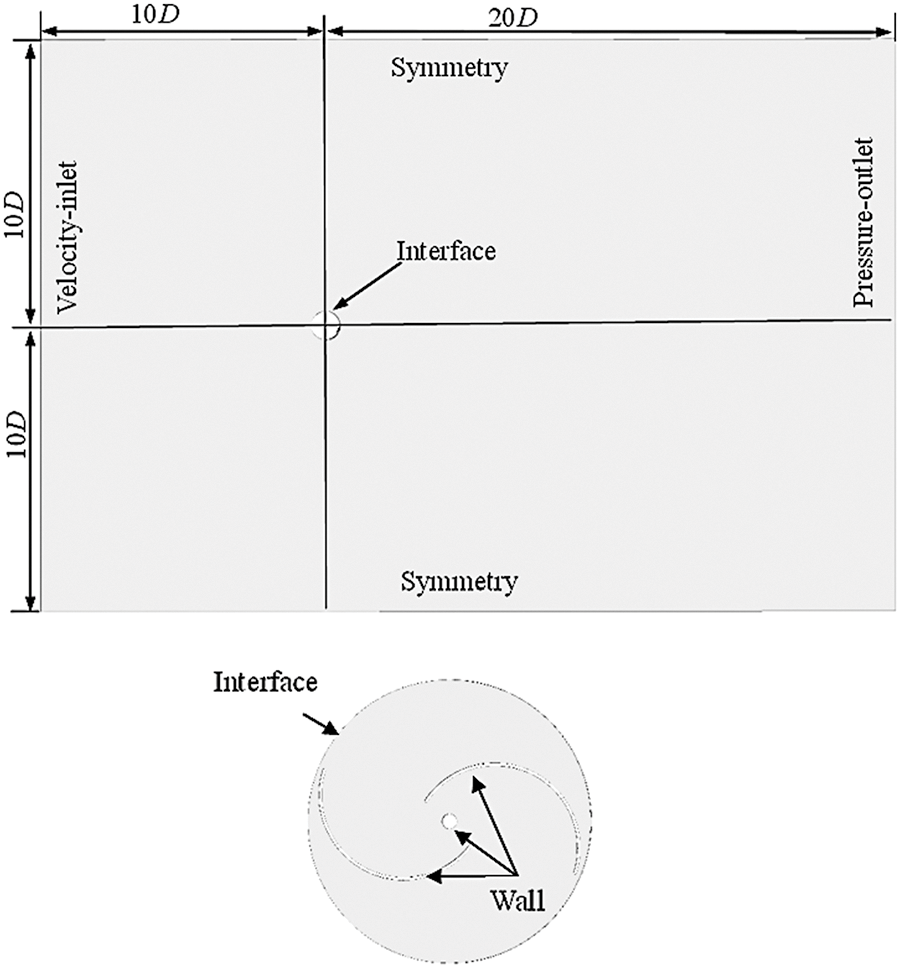
Figure 1: Multi-block computational domains showing dimensions and boundary conditions

The relationship between the power coefficient of the Savonius turbine and the blade geometry is studied. Therefore, we define the control parameters of blade clearance, such as the blade overlap ratio β, blade clearance ratio ε, blade circumferential angle γ, here the circumferential angle γ of the blade is limited to the circular blade, blade tip velocity ratio γ, arc radius ratio δ and dimensionless turbine power coefficient Cp. The relationship between the control parameters of blade geometry and the turbine power coefficient Cp is studied under the condition of inlet velocity of 0.8 m/s. As this paper is based on computational fluid dynamics to optimize the blade shape of the Savonius turbine, it should be noted that the study excludes the consideration of the blockage in the flow channel.

In the design of runner blades, the shape and parameter values of the turbine model used in this study are shown in Fig. 2 and Table 1. The blade tip velocity ratio λ is defined as following Eq. (1):

λ=ωD2U0(1)

where ω is the angular velocity of runner, D is the diameter of runner, and U0 is the inlet velocity. The blade tip ratio β is defined according to the following Eq. (2) :

β=eD(2)

The blade clearance ratio ε is defined according to the following Eq. (3):

ε=aD(3)

The arc radius ratio δ is defined according to the following Eq. (4):

δ=RbD(4)

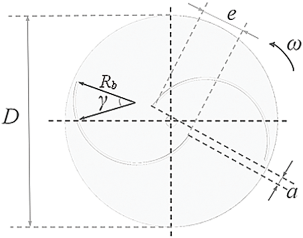
Figure 2: Geometric parameters of turbine

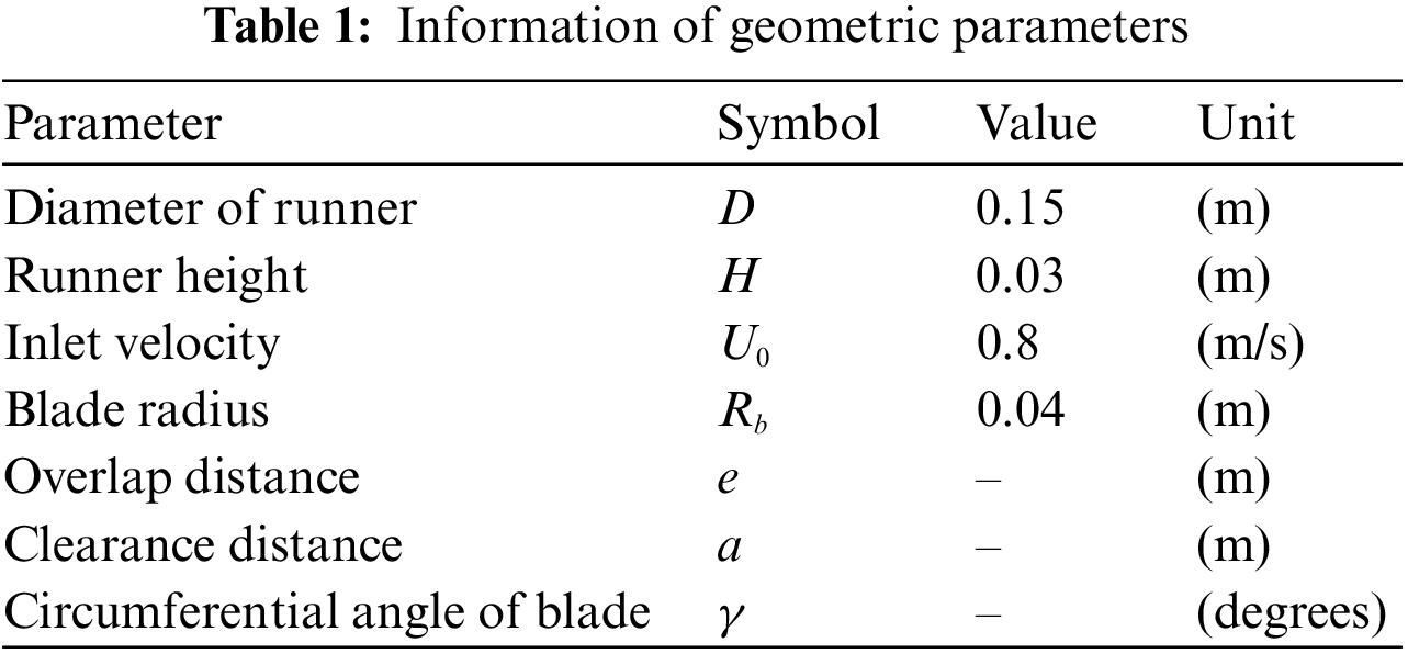
Parameters e, a, Rb are shown in Fig. 2 above. D is the diameter of runner.

3  Performance Evaluation of Baseline Model

3.1 CFD Setup

In this study, the commercial software ANSYS CFX was used for CFD simulation. The fluid medium was water at 25°C, and the pressure was 1 Atm. The turbulence model utilized was the SST k-ω model, which is more accurate and reliable and widely applied. In CFD simulation, one side of the domain was taken as the inlet and the other side was taken as the outlet. The condition of the velocity inlet type was set at the inlet side, while the static pressure type outlet boundary was set at the outlet side. All wall boundaries use the no-slip wall conditions. The Multiple Reference Frame (MRF) is used. The computational domain consists of the stationary domain and the rotational domain, and the boundary between the stationary and the rotational domain is given as the interface. Steady state iterative simulation is performed first. The steady results are used as the basis for the unsteady state simulation. The convergent criterion is that the RMS residual of the continuity equation and momentum equation was less than 0.0001.

3.2 Grid Preparation and Check

To conduct CFD simulation, grid preparation and grid-independent checking should be carried out. The grid of the computational domain is shown in Fig. 3. In order to ensure the accuracy of CFD, four sets of different grids (N1, N2, N3 and N4) are prepared with the number of grids of 10 thousand, 20 thousand, 40 thousand, 80 thousand, respectively. The performance of the Savonius turbine under the same operating condition is tested by using these four sets of grids. The grid check results are shown in Fig. 4. From the different grid of turbine performance variation curves, the error is within the permissible range. Finally, the grid of 20 thousand nodes is selected for CFD simulation.

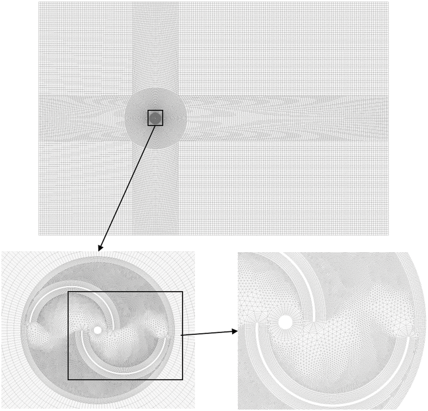
Figure 3: Grid of computational domain

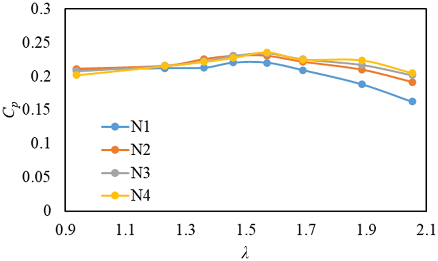
Figure 4: Grid independence check details

3.3 Performance Evaluation and Comparison

In Fig. 5, we performed CFD numerical simulations of the model and compared the CFD prediction results with Nakajima’s experimental results [36]. It is found that the fitting is good from the trend of power coefficient, but the value of power coefficient Cp is relatively low; these errors may be due to differences in model size. Therefore, the numerical model can be used to simulate the operation of the Savonius turbine at low flow velocity. As shown in Fig. 5 below, the power coefficient Cp rises slowly when λ is smaller than 1.1, and then decreases slowly when λ is bigger than 1.1.

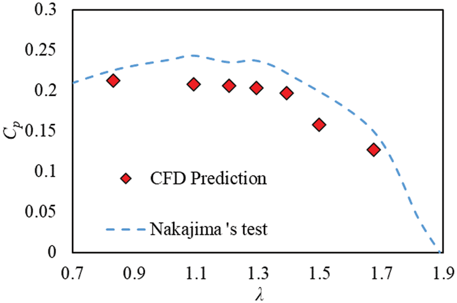
Figure 5: Comparison of power coefficients Cp of CFD prediction and Nakajima’s test

4  Runner Blade Geometry Optimization

4.1 Parameterization and Coding

In this paper, the key optimization parameters are blade overlap ratio β, clearance ratio ε, and blade circumference angle γ. Before the genetic algorithm optimization, it is necessary to carry out binary coding for the parameters above. In this study, the range of blade overlap ratio β is 2~2.5, the range of clearance ratio ε is −0.2~0.2 and the range of the blade circumference angle γ is 0~30. The precision of the three parameters is 0.2001, 0.0015 and 0.1176, respectively. Thus, an 8-bit binary code string is chosen to describe a parameter, so that an individual contains a 24-bit binary code. By selecting 10 individuals as a generation, a total of 10 generations of genetic manipulation were performed in order to finally obtain the best individual.

4.2 Objective Function

In this paper, the optimal power coefficient and maximum power coefficient area width of the Savonius turbine are analyzed and optimized, so define the dimensionless number power coefficient Cp according to Eq. (5):

Cp=2TωρHDU03(5)

where T is the torque, ω is the rotor angular velocity, ρ is the fluid density, H is the runner height, D is the runner diameter, and U0 is the steady inlet velocity.

Define the optimal power coefficient is Cpmax, the width of optimal power coefficient R is defined as the range of the tip speed ratio λ corresponding to 90% or more of the optimal power coefficient Cpmax. Cpmax and R are used as the objective function to judge the performance of Savonius turbine, and construct the performance weighting functions W as following Eq. (6):

W=Cpmaxw1c1+Rw2c2(6)

where w1is the weight of Cpmax of 0.5, c1 is the maximum experimental power coefficient value of 0.3, w2 is the weight of R of 0.5, and c2 is the range of the maximum tip speed ratio of 2. In order to make the Savonius turbine have better operating power, and to operate efficiently and permanently under overall conditions, w1 and w2 are set to 0.5 and 0.5.

4.3 Setup of GA

The optimization parameters had previously been binary coded, followed by genetic algorithm (GA) operations that set the probability of crossover at 20%, the probability of variation at 5%, and the probability of copying/eliminating the best/worst individuals at 100%. The flow chart illustrating this process is drawn in Fig. 6 below. On the basis of this configuration in place, the optimization design is carried out combined with CFD simulation.

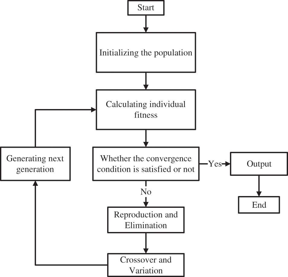
Figure 6: Flow chart of genetic algorithm operation

5  Comparative Analysis

5.1 Geometry Comparison

Compare the blade geometry of the initial scheme with the optimal scheme, as shown in Fig. 7 below. The initial scheme has the following parameters: β = 0.2, ε = 0, γ = 0°. The blade parameters of the optimal scheme are β = 0.202157, ε = 0.179608, γ = 27.64706°. From the data and the figure below, it can be seen that the circumferential angle of the blade decreases by approximately 27°, the overlap ratio experiences a modest increase, and the gap ratio noticeably increases. The optimization of the blade geometry of the Savonius turbine further enhances the operation performance of the turbine and is well-adapted for the overall working conditions.

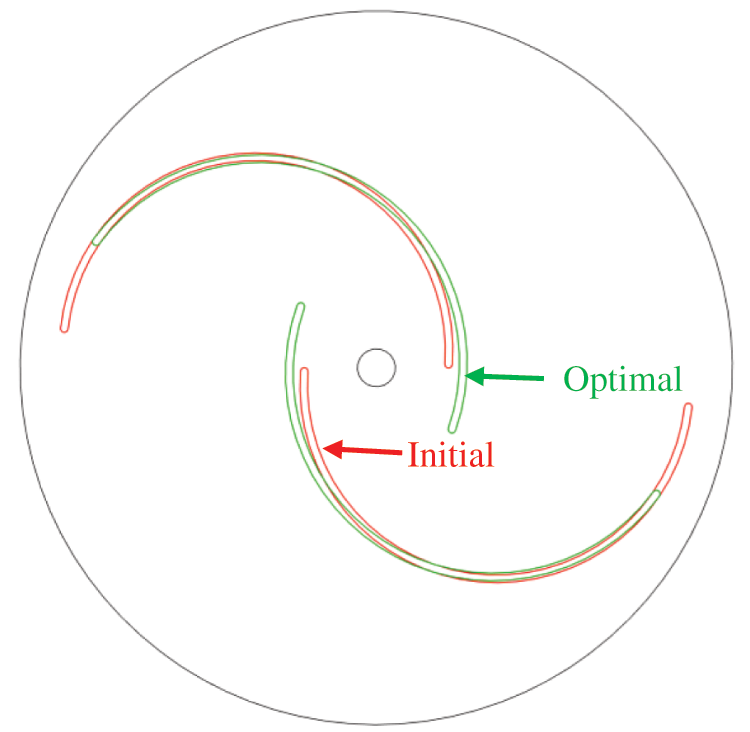
Figure 7: Comparison of blade geometry before and after optimization

5.2 Performance Comparison

The performance of the turbine with the optimized blade is compared with the that of the turbine with the initial blade, as shown in Fig. 8. The overall performance of the optimal Savonius turbine is superior to the initial turbine. In the initial scheme, the power coefficient Cp rises gently before the blade tip velocity ratio λ = 1.1, then falls slowly before λ = 1.5 and falls sharply after λ = 1.5. Finally, the power coefficient Cp drops to around 10%. However, the power coefficient Cp of the optimal scheme rises continuously until the blade tip velocity ratio λ = 1.5, and then falls after the blade tip velocity ratio λ = 1.5, but it ends up at about 22.5%. The performance improvement of the Savonius turbine is very obvious.

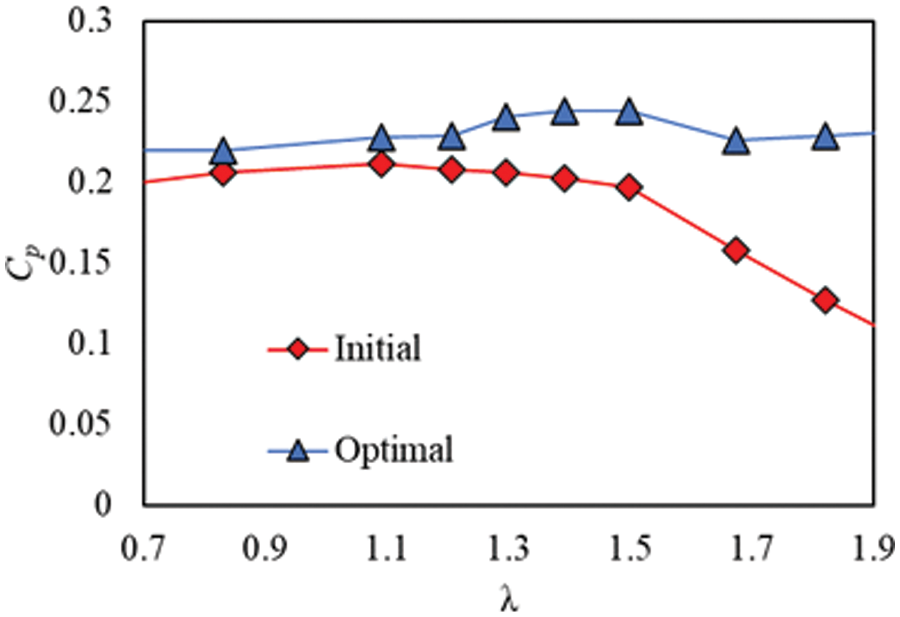
Figure 8: Comparison of Savonius turbine’s performance of initial and optimal scheme

The fluctuation curves of the power coefficient Cp before and after blade optimization were analyzed. Condition with (a) λ = 0.831 of Fig. 9 shows that the fluctuation peak value of the initial scheme was significantly higher than that of the optimal scheme, but it is also clear from the figure that the value Cp of the optimal scheme is always higher than that of the initial scheme in the upward region. The descending area is sometimes higher and lower than that of the initial scheme. Condition (b) with λ = 1.207 of Fig. 9 indicates that it is obvious that the optimal scheme is higher than the initial scheme both in the upward region and the peak value, while the descending area is slightly lower than that of the initial scheme. Condition (c) with λ = 1.674 of Fig. 9 reveals that the fluctuation curve of the optimal scheme is more pronounced, which is basically consistent with the trend of Fig. 9b. To sum up, the Cp of the runner blade is also changing at different times of rotation and it changes periodically. Therefore, the power coefficient of this turbine needs to be analyzed at different times of operation.

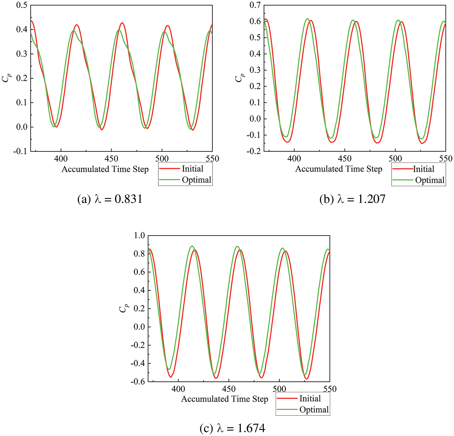
Figure 9: The comparison of the Cp fluctuating curves of the initial and optimal scheme under three conditions

5.3 Flow Pattern Comparison

In this paper, the energy loss analysis based on the entropy production rate of the Savonius turbine is carried out. The entropy production rate Ep is defined as Eq. (7):

Ep=β1ρω1kT1(7)

where β1 is the model closure constant, given β1 = 0.09, ω1 is the turbulent eddy frequency, k is the turbulent energy, ρ is the fluid density, and T1 is the temperature.

The initial scheme and optimal scheme of blade rotation are examined at different locations under various working conditions. Conditions like blade tip velocity ratio λ = 0.831, λ = 1.207, λ = 1.674 are discussed. Fig. 10 shows the position of the blade rotation angles, applied to 36°, 72°, 108°, 144° and 180°. Define the moment of motion of the runner blades T∗ followed as Eq. (8):

T∗=πint(8)

where π is circumference ratio, i is the number of segments in a π cycle, nt is the number of segments through which the blade passes.

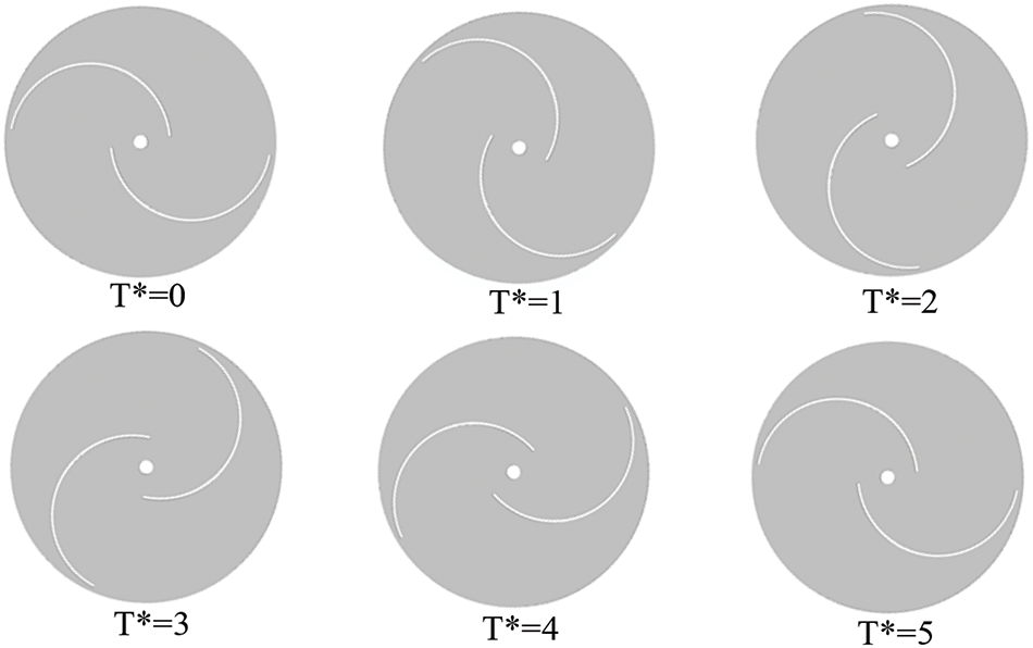
Figure 10: The position of the runner blades at five moments

Fig. 11 shows the condition of λ = 0.831 and T∗ = 1. The blade leading edge is defined as the end near the rotating shaft, the blade trailing edge is defined as the end near the interface. It can be seen from Fig. 11 that Blade A runs well before optimization, with no obvious energy loss, only a slight energy loss at the leading edge. Blade B’s leading edge and trailing edge have some energy losses, especially at the trailing edge part. After optimization, Blade A has a slight energy loss, and Blade B’s energy loss is significantly reduced, about 98%.

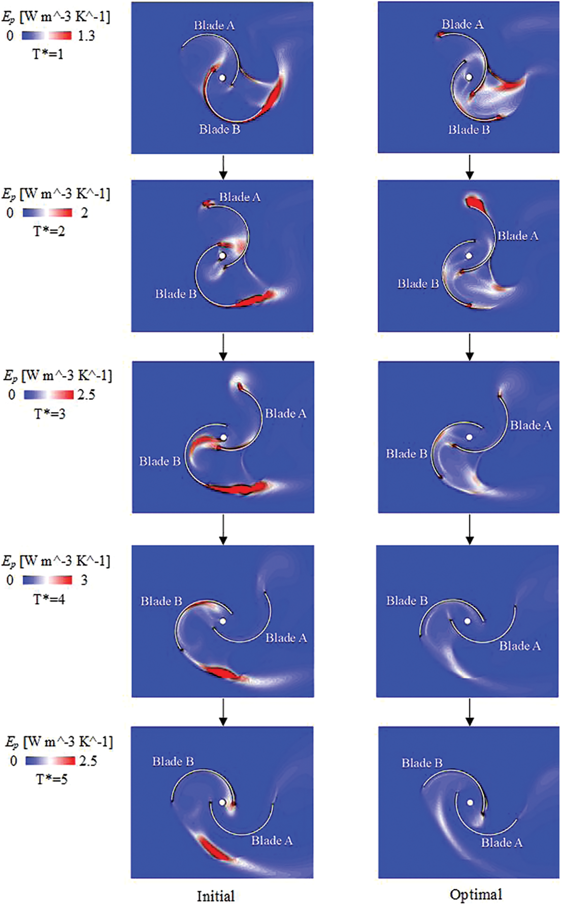
Figure 11: The comparison of the entropy production rate of initial and optimal schemes at five moments when λ = 0.831

When T∗ = 2. Before optimization, there is a slight energy loss at the leading edge of Blade A, and the energy loss at the trailing edge is bigger than that at the leading edge. There is a slight energy loss at the leading edge of Blade B, but a big energy loss at the trailing edge, which is about 10 times that of the leading edge. After optimization, there is a slight energy loss at the leading edge of Blade A, but the energy loss at the trailing edge increases greatly, about 5 times of that before optimization. Blade B has almost no energy loss, much less than that before optimization.

When T∗ = 3. Before optimization, there is a part of energy loss at the leading edge of Blade A and in front of it, and a small loss at the trailing edge. There is no energy loss at the leading edge of Blade B, and a large amount of energy loss is produced at the trailing edge of Blade B. After optimization, there is an energy loss part at both the leading and trailing edges of Blade A, which is in the shape of a dot. There is no energy loss at the leading edge of Blade B, and there is a slight dot-like energy loss at the trailing edge, which is weaker than that before optimization.

When T∗ = 4. Before optimization, Blade A runs in good condition with no energy loss. There is no obvious energy loss at the leading and trailing edge of Blade B, but there is a large energy loss area behind the trailing edge. After optimization, Blades A and B run in good condition, with almost no energy loss, there is a slight energy loss behind the Blade B trailing edge, which is significantly weaker compared with that before optimization.

When T∗ = 5. Before optimization, Blade A has a good performance with no energy loss. There is a dot-like energy loss at the leading edge of Blade B, but there is a large energy loss area behind the trailing edge. After optimization, Blades A and B operate well, with almost no energy loss. The leading and trailing edge of Blade B have a slight energy loss. The big energy loss before optimization almost disappeared.

Fig. 12 shows the condition of λ = 1.207 and T∗ = 1. Before optimization, Blade A ran in good condition with no energy loss. There was a dot-like energy loss at the leading edge of Blade B, but there was also a thin arc-like energy loss area at the trailing edge and the convex side of Blade B. After optimization, the energy loss in the leading edge of Blade A was increased, and Blade B was in good condition with almost no energy loss. There was a small energy loss in the leading edge and trailing edge of Blade B, but it became small compared to what it was before it was optimized.

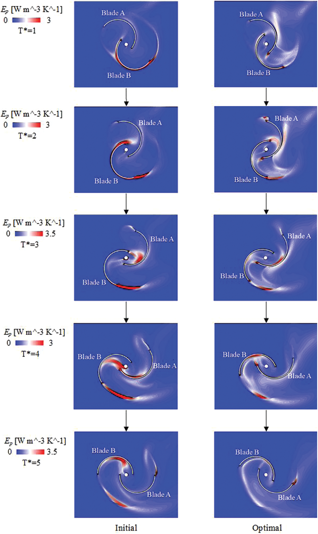
Figure 12: The comparison of the entropy production rate of initial and optimal schemes at five moments when λ = 1.207

When T∗ = 2. Before optimization, Blade A ran in good condition with no energy loss. There were strip energy loss regions at the leading and trailing edge of Blade B. After optimization, the energy loss at the leading edge of Blade A was increased, and the energy loss at the leading edge of Blade B was reduced to a dot-like area. The energy loss at the trailing edge and rear of Blade A was decreased, but it was still a thin strip.

When T∗ = 3. Before optimization, Blade A operated well, there was a certain degree of energy loss in the concave side of Blade A near the leading edge. There was a strip-like energy loss area at the front and trailing edge of Blade B, in which the energy loss behind the trailing edge was larger, and the distribution was linear. After optimization, the energy loss at the leading edge of Blade A increased; the energy loss at the trailing edge of Blade B decreased to a dot-like area, and the energy loss at the rear of the trailing edge decreased, but it was still a thin strip.

When T∗ = 4. Before optimization, there were circular and thin strip energy loss regions at the leading edge and concave side of Blade A, thick and long strip energy loss regions at the trailing edge of Blade B, and a small spiral energy loss region at the concave side of Blade A. After optimization, the energy loss at the leading edge of Blade A was approximately unchanged, the energy loss at the trailing edge of Blade B was reduced to a short strip, and the small spiral energy loss at the concave side of Blade B was also reduced to a short arc.

When T∗ = 5. Before optimization, there was a circular arc energy loss at the leading edge of Blade A, a good condition at the trailing edge of Blade B, a thin strip energy loss area at the trailing edge of Blade B, and a slightly thick arc energy loss area at the concave side of Blade B. After optimization, the energy loss of Blade A showed no significant reduction, the energy loss of Blade B reduced obviously.

Fig. 13 shows the condition of λ = 1.674 and T∗ = 1. Before optimization, there was a slight energy loss at the trailing edge of Blade A and a small energy loss area at the trailing edge of Blade B. There was a certain energy loss at the convex side surface of Blade B. After optimization, the energy loss at the trailing edge of Blade A was obviously decreased, but the energy loss at the leading edge was slightly increased, and the energy loss at the convex side of Blade B was obviously reduced, but there was still a 25% blade-size energy loss area.

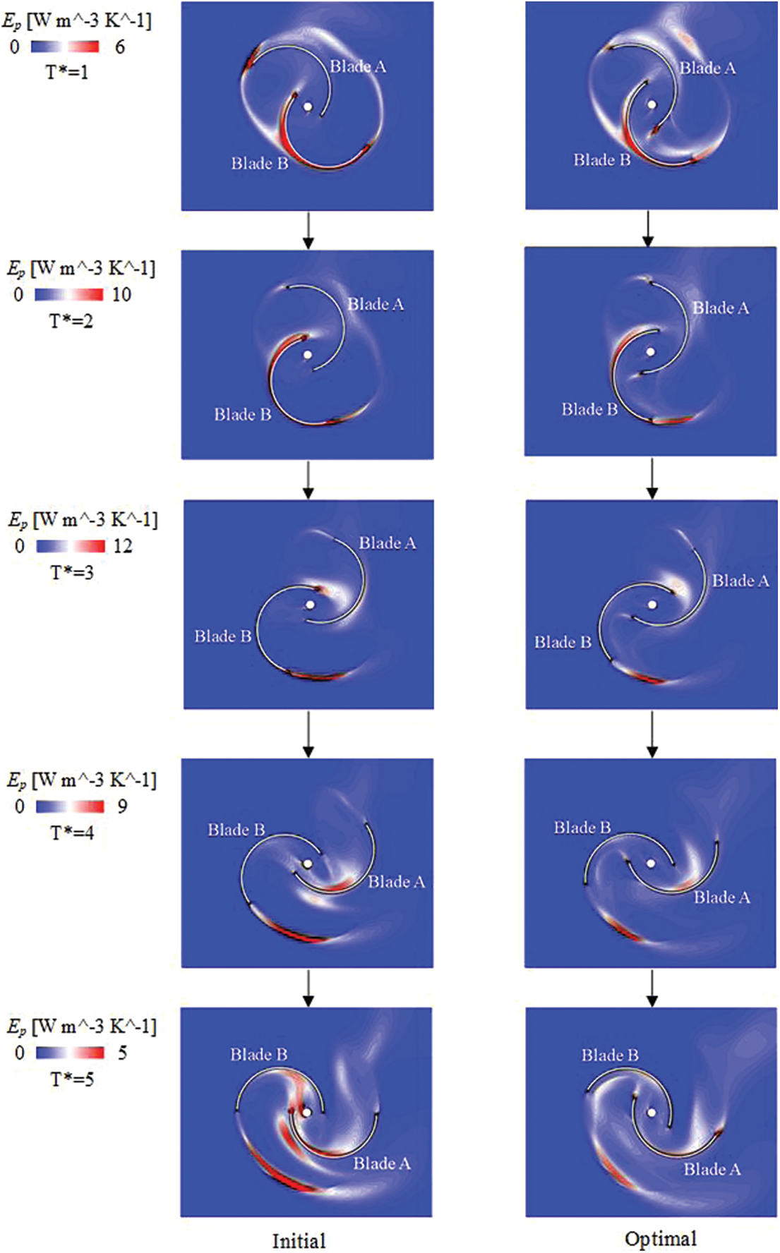
Figure 13: The comparison of the entropy production rate of initial and optimal schemes at five moments when λ = 1.674

When T∗ = 2. Before optimization, Blade A was in good condition with no obvious energy loss, Blade B had a slight energy loss at the leading and trailing edge, and some energy loss was produced on the convex side surface of Blade B. After optimization, there was a slight increase in energy loss at the leading and trailing edges of Blade A, a slight increase in energy loss at the trailing edges of Blade B and its rear slender strips, and a significant decrease in energy loss at the convex side of Blade B, but there is still a 15% blade-sized area of energy loss.

When T∗ = 3. Before optimization, Blade A was in good condition with no obvious energy loss, and there was a slight energy loss at the leading and trailing edges of Blade B, and there was a fine arc-shaped energy loss area behind the tail edge. After optimization, Blade A remains in a state of no apparent energy loss, and the length of energy loss behind Blade B’s trailing edge is obviously shortened.

When T∗ = 4. Before optimization, the leading and trailing edges of Blade A were in good condition with no obvious energy loss, but there was a certain degree of energy loss near the concave side of the leading edge, and there was a slight energy loss at the trailing edge of Blade B, and there is a long arc-shaped energy loss region behind the trailing edge. After optimization, the energy loss of Blade A’s concave side is obviously weakened, and the energy loss length behind Blade B’s trailing edge is obviously shortened.

When T∗ = 5. Before optimization, there was circular spot energy loss at the front and trailing edge of Blade A, circular arc energy loss at both sides of Blade B, and slender circular arc energy loss area at the rear of Blade B’s trailing edge. After optimization, the energy loss of Blade A’s concave side is obviously weakened, and the energy loss length behind Blade B trailing edge is obviously shortened.

6  Conclusions

The main conclusions of this study are as follows:

(1) In this paper, before optimization, the power coefficient of the turbine in the original scheme increases slightly with the increase of the blade tip speed ratio from 0.7 to 1.1, then it decreases slowly, and finally decreases sharply to 10% at λ = 1.9. After optimization, the power coefficient of the turbine in the original scheme experiences a modest increase to approximately about 24% and decreases to about 22.5%. Before optimization, the turbine power coefficient peaks at a blade tip speed ratio λ = 1.1, and after optimization, it reaches the peak at λ = 1.5. From the change in power coefficient of the Savonius turbine, its performance optimization has improved significantly. The overall performance of the optimized turbine is higher than before the optimization. The power coefficient Cp remains fairly constant over the range of λ studied. This is highly significant.

(2) In this paper, a Genetic Algorithm (GA) was used to optimize the blade overlap ratio β, blade clearance ratio ε and circumference angle γ at 0.2~0.25, −0.2~0.2 and 0~30°, respectively, and verified with computational fluid dynamics (CFD). Optimal: β = 0.2021, ε = 0.1796, γ = 27.647°, initial: β = 0.2, ε = 0, γ = 0°. β increased by 0.0215, ε increased by 0.1796 and γ increased by 27.647°. the optimized turbine blade increases the circumference angle by about 30° near the rotating shaft, but decreases the circumference angle by about 30° near the interface. After optimization, the maximum power coefficient Cpmax of the Savonius hydrokinetic turbine is increased from 21.48% to 24.5%, and the width of the high-power coefficient zone R is also increased from 0.73 to 1.02.

(3) In this paper, the energy loss of the optimized turbine, especially around the runner blades, is obviously reduced. The five moments (T∗ = 1, 2, 3, 4 and 5) of the runner running in the initial and optimal conditions are analyzed and compared. The energy loss is reduced by about 95% under the condition of λ = 0.831, the energy loss is reduced by about 90% under λ = 1.207, and the energy loss is reduced by about 85% under λ = 1.674. The reduction in energy loss from the blades corresponds to an increase in the power coefficient.

Acknowledgement: We acknowledge the financial support of National Natural Science Foundation of China to support the research.

Funding Statement: This research was funded by National Natural Science Foundation of China, Grant Number 52079142.

Author Contributions: The authors confirm contribution to the paper as follows: study conception and design: Zhang F. F., Guang W. L.; data collection: Wu Y. Z.; analysis and interpretation of results: Tao R., Li X. Q.; draft manuscript preparation: Lu J. H., Tao R. All authors reviewed the results and approved the final version of the manuscript.

Availability of Data and Materials: Data supporting this study are included within the article.

Conflicts of Interest: The authors declare that they have no conflicts of interest to report regarding the present study.

References

1. Fabre, A., Fodha, M., Ricci, F. (2020). Mineral resources for renewable energy: Optimal timing of energy production. Resource and Energy Economics, 59, 101131. [Google Scholar]

2. Holechek, J. L., Geli, H. M. E., Sawalhah, M. N., Valdez, R. (2022). A global assessment: Can renewable energy replace fossil fuels by 2050. Sustainability, 14(8), 4792. [Google Scholar]

3. Chamberland, A., Levesque, S. (1996). Hydroelectricity, an option to reduce greenhouse gas emissions from thermal power plants. Energy Conversion and Management, 37(6–8), 885–890. [Google Scholar]

4. Schwartz, F. H., Shahidehpour, M. (2006). Small hydro as green power. 2006 IEEE EIC Climate Change Conference, pp. 1–6. Ottawa, Canada. [Google Scholar]

5. Tapia, A., Millan, P., Gomez-Estern, E. (2018). Integer programming to optimize micro-hydro power plants for generic river profiles. Renewable Energy, 126, 905–914. [Google Scholar]

6. Rengma, T. S., Sengupta, A. R., Basumatary, M., Biswas, A., Bhanja, D. (2021). Performance analysis of a two bladed Savonius water turbine cluster for perennial river-stream application at low water speeds. Journal of the Brazilian Society of Mechanical Sciences and Engineering, 43(5), 1–21. [Google Scholar]

7. Güney, M. S., Kaygusuz, K. (2010). Hydrokinetic energy conversion systems: A technology status review. Renewable & Sustainable Energy Reviews, 14(9), 2996–3004. [Google Scholar]

8. Khan, A. A., Shahzad, A., Hayat, I., Miah, M. S. (2016). Recovery of flow conditions for optimum electricity generation through micro hydro turbines. Renewable Energy, 96, 940–948. [Google Scholar]

9. Song, L., Liu, H. Z., Yang, Z. X., Dong, G. Q. (2016). Simulation analysis based performance comparison for vertical axis wind turbines. 2016 International Conference on Advanced Mechatronic Systems (ICAMechS), pp. 334–339. Melbourne, Australia. [Google Scholar]

10. Song, L., Liu, H. X., Yang, Z. X. (2015). Performance comparison for Savonius type wind turbines by numerical analysis approaches. 2015 International Conference on Advanced Mechatronic Systems (ICAMechS), pp. 402–407. Beijing, China. [Google Scholar]

11. Thiyagaraj, J., Rahamathullah, I., Anbuchezhiyan, G., Barathiraja, R., Ponshanmugakumar, A. (2021). Influence of blade numbers, overlap ratio and modified blades on performance characteristics of the Savonius hydro-kinetic turbine. Materials Today: Proceedings, 46, 4047–4053. [Google Scholar]

12. Bian, P. X., Yang, Z. H., Wang, Y., Ma, P. L., Wang, S. Y. (2018). Hydrodynamic performance of Savonius water turbine. Journal of Zhejiang University Engineering Science, 52(2), 268–272. [Google Scholar]

13. Kumar, R. S., Premkumar, T. M., Seralathan, S., Xavier, D. D., Elumalai, E. S. et al. (2020). Simulation studies on influence of shape and number of blades on the performance of vertical axis wind turbine. Materials Today: Proceedings, 33(3), 3616–3620. [Google Scholar]

14. Mosbahi, M., Lajnef, M., Derbel, M., Mosbahi, B., Driss, Z. et al. (2021). Performance improvement of a Savonius water rotor with novel blade shapes. Ocean Engineering, 237(1), 109611. [Google Scholar]

15. Hashem, I., Zhu, B. S. (2021). Metamodeling-based parametric optimization of a bio-inspired Savonius-type hydrokinetic turbine. Renewable Energy, 180(6), 560–576. [Google Scholar]

16. Wang, W., Song, B. W., Mao, Z. Y., Tian, W. L. (2019). Optimization of Savonius wind turbine impeller with bilateral contour. Journal of Harbin Engineering University, 40(2), 254–259. [Google Scholar]

17. Shashikumar, C. M., Vijaykumar, H., Vasudeva, M. (2021). Numerical investigation of conventional and tapered Savonius hydrokinetic turbines for low-velocity hydropower application in an irrigation channel. Sustainable Energy Technologies and Assessment, 43, 100871. [Google Scholar]

18. Shashikumar, C. M., Honnasiddaiah, R., Hindasageri, V., Madav, V. (2021). Studies on application of vertical axis hydro turbine for sustainable power generation in irrigation channels with different bed slopes. Renewable Energy, 163, 845–857. [Google Scholar]

19. Khani, M. S., Shahsavani, Y., Mehraein, M., Kisi, O. (2023). Performance evaluation of the Savonius hydrokinetic turbine using soft computing techniques. Renewable Energy, 215, 118906. [Google Scholar]

20. Wu, Y. Z., Guang, W. L., Tao, R., L, J., Xiao, R.F. (2023). Dynamic mode structure analysis of the near-wake region of a Savonius-type hydrokinetic turbine. Ocean Engineering, 282(1), 114965. [Google Scholar]

21. Wang, X. L., Zhu, Z. Q., Liu, Z., Wu, Z. C. (2006). Bi-point/bi-objective optimization design of ailfoil using N-S equations. Journal of Beijing University of Aeronautics and Astronautics, 32(5), 503–507. [Google Scholar]

22. Dong, X., Liu, X. M. (2019). Bi-objective topology optimization of asymmetrical fixed-geometry microvalve for non-Newtonian flow. Microsystem Technologies Micro and Nanosystems-Information Storage and Processing Systems, 25(6), 2471–2479. [Google Scholar]

23. Chan, C. M., Bai, H. L., He, D. Q. (2018). Blade shape optimization of the Savonius wind turbine using a genetic algorithm. Applied Energy, 213(6), 148–157. [Google Scholar]

24. Jia, R. Y., Xia, H. J., Zhang, S., Su, W. G., Xu, S. H. (2022). Optimal design of Savonius wind turbine blade based on support vector regression surrogate model and modified flower pollination algorithm. Energy Conversion and Management, 270(5), 116247. [Google Scholar]

25. Mohamad, B., Shahram, D., Jamal, S. (2019). Design optimization of a centrifugal pump using particle swarm optimization algorithm. International Journal of Fluid Machinery and Systems, 12(4), 322–331. [Google Scholar]

26. Oyama, A., Liou, M. S. (2002). Multiobjective optimization of rocket engine pumps using evolutionary algorithm. Journal of Propulsion and Power, 18(3), 528–535. [Google Scholar]

27. Wu, G. W., Wu, H., Wang, X. Y., Zhou, Q. W., Liu, X. M. (2018). Tidal turbine array optimization based on the discrete particle swarm algorithm. China Ocean Engineering, 32(3), 358–364. [Google Scholar]

28. Han, Z., Wu, T. (2008). Optimal design of wind turbine blades based on genetic algorithm. Journal of Power Engineering, 28(6), 955–958. [Google Scholar]

29. Lu, J. H., Zhang, F. F., Tao, R., Li, X. Q., Zhu, D. et al. (2023). Optimization of runner and vane blade angle of an oscillating water column based on genetic algorithm and neural network. Ocean Engineering, 284(4), 115257. [Google Scholar]

30. Chang, H., Shi, W. W., Li, W., Liu, J. R. (2019). Energy loss analysis of novel self-priming pump based on the entropy production theory. Journal of Thermal Science, 28(2), 306–318. [Google Scholar]

31. Su, X., Jin, W., Zu, Z., Li, Z., Jia, H. (2021). Performance characteristics and energy loss analyses of a high-speed centrifugal pump with straight blades. Journal of Applied Fluid Mechanics, 14(5), 1377–1388. [Google Scholar]

32. Ghorani, M. M., Haghighi, M. H. S., Maleki, A. (2020). A numerical study on mechanisms of energy dissipation in a pump as turbine (PAT) using entropy generation theory. Renewable Energy, 162(1), 1036–1053. [Google Scholar]

33. Wang, Z. L., Luo, W., Zhang, B. W., Asomani, S. N., Xu, J. et al. (2022). Performance analysis of geometrically optimized PaT at turbine mode: A perspective of entropy production evaluation. Proceedings of the Institution of Mechanical Engineers, Part C: Journal of Mechanical Engineering Science, 236(24), 11446–11463. [Google Scholar]

34. Sakamoto, S., Murakami, S., Mochida, A. (1993). Numerical study on flow past 2D square cylinder by large eddy simulation: Comparison between 2D and 3D computations. Journal of Wind Engineering and Industrial Aerodynamics, 50, 61–68. [Google Scholar]

35. Franchina, N., Persico, G., Savini, M. (2019). 2D-3D computations of a vertical axis wind turbine flow field: Modeling issues and physical interpretations. Renewable Energy, 136(8), 1170–1189. [Google Scholar]

36. Nakajima, M., Iio, S., Ikeda, T. (2008). Performance of Savonius rotor for environmentally friendly hydraulic turbine. Journal of Fluid Science and Technology, 3(3), 420–429. [Google Scholar]