Distributed Robust Optimal Dispatch for the Microgrid Considering Output Correlation between Wind and Photovoltaic

Nomenclature

Indices

Parameters

Variables

1  Introduction

In recent years, renewable resources such as wind and solar have been incorporated into the grid on a large scale through the form of the microgrid (MG) to ease the growing energy crisis and environmental pressure. MG is a comprehensive power distribution system [1] with distributed power supply, energy storage device, and load as the main body. However, the uncertainty of distributed power generation (DG) output poses a great challenge to the security of the system [2].

The deterministic optimization model has a simple form, but the scheduling results are influenced by uncertainty [3]. To solve the uncertainty of DG output, current research mainly focuses on stochastic programming and robust optimization. Stochastic optimization assumes that the output of renewable energy can meet a certain probability distribution, and selects a large number of typical scenarios in the actual operation for optimization. This method applies to the scenario with the probability of the uncertainty parameters considered [4]. However, because of the complexity of factors affecting variable uncertainty, this method generally does not accurately reflect the actual pattern. Robust optimization does not consider the statistics of random variables, and only obtains the interval information of random variables. This method uses uncertain sets to describe the possible range of random variables and minimizes the running cost of the random variables in the worst scenarios [5]. However, the optimization results are often somewhat conservative, resulting in a poor economy [6]. To compensate for the limitations of these two methods, distributed robust optimization (DRO) is proposed. By building a reasonably distributed fuzzy set of random variables and looking for the worst probability distribution, DRO addresses the problems of data scarcity and the difficulty of accurately describing random distributions in random programming methods, as well as the conservative results of robust optimization. Traditional DRO is mostly based on the Wasserstein metric or the corresponding moment information to construct the probability distribution set [7–9]. After obtaining complex non-deterministic polynomial problems, simplify and solve them [10]. To avoid solving complex dual problems, we can obtain the historical data of many systems by data-driven methods; and bound the confidence interval by using norms.

Literature [11] adopted the stochastic planning method to generate a large number of discrete scenarios to represent the uncertainty of DG output and load based on the scenarios method, then transformed the uncertainty problem into a deterministic problem treatment. Literature [12] used tunable robust optimization to establish the worst scenarios set to characterize the uncertainty of wind power; then transformed the model into a linear model by linear optimization strong dual theory. Based on Literature [12–13] added power to gas devices to the microgrid system to improve the wind and solar power accommodation, then built a two-stage DRO model considering both economy and environmental protection. Literature [14] used the adaptive robust optimization method to characterize the uncertainty of DG and load; then used the tri-layer decomposition algorithm of the original and dual-cut planes to optimally configure the DG in the distribution network. However, most of the above documents ignore the correlation between wind power and photovoltaic output. And there are nonlinear terms in the model, which makes the solution more complex and time-consuming.

Given the above defects, some scholars have carried out research on solar-wind correlation. According to the literature [15], Pearson Coefficient was utilized as a measure of the correlations between the wind turbine power deviations, and the time constraint. The threshold of certain conditions was used to establish the uncertainty of considering the time correlation of a single Wind turbine output at different moments and the spatial correlation between multiple Wind turbines. However, Pearson Coefficient is a linear correlation coefficient, which is difficult to apply to nonlinear monotone transformation. Literature [16] used Spearman and Kendal correlation coefficients to describe the correlation between wind speed and wind output of two wind farms, and various Copula functions were used to model the joint distribution. Then two-stage maximum likelihood estimation was used to estimate the unknown parameters, but the correlation was not extended to the solar and wind power. Considering the different characteristics of different Copula functions, literature [17] proposed a method of generating wind and solar scenarios based on nonparametric kernel density estimation and combined Copula functions, then obtained the uncertainty and correlation sequence of wind power and solar power generation in a typical day. However, due to the selection of multiple functions, the solution would be relatively complicated. Literature [18] further selected the Frank-Copula function as the connection function to deal with solar-wind correlation, but the uncertainty probability distribution of the generated scene is not constrained.

This paper establishes a distributed robust optimization model for the Microgrid which considers the correlation of wind and solar power output and the probability distribution constraints. The main contributions of this paper are as follows:

(1) A method to generate scenarios of wind and solar power output using non-parametric kernel density estimation and Frank-Copula functions is proposed. The uncertainty and correlativity of wind and solar power output can be better described by kernel density estimation than by parametric estimation.

(2) A two-stage distributed robust optimization model is constructed and combines the 1-norm and ∞-norm while constraining the confidence set of the uncertainty probability distribution. The column and constraint generation algorithm is used to solve the problem.

Other sections of this paper are organized as follows. The framework flowchart of the DRO method is proposed in the Second Section. The Third Section presents the generation and reduction of wind and solar power scenarios. The MG deterministic model considering multiple scenarios is established in the Fourth Section and the distributed robust optimization model for MG is established in the Fifth Section. The Sixth Section provides illustrative examples and analysis. Conclusions are given in the Seventh Section.

2  Framework Flowchart of the DRO Method

A multi-scenario DRO method is proposed with consideration of the multiple uncertainties of wind and solar power output. The framework flowchart of the proposed method is illustrated in Fig. 1. Firstly, scenarios of wind and solar power output are generated based on non-parametric kernel density estimation and the Frank-Copula function; then the generated scenario results are reduced by K-means clustering; finally, the probability confidence interval of scenario distribution is constrained by 1-norm and ∞-norm. The model is solved by a column-and-constraint generation (C&CG) algorithm.

Figure 1: Framework flowchart of the multi-scenario DRO method

3  Scenarios Generation and Reduction

The distributed robust optimization method based on scenario probability distribution has high requirements for both the number of scenarios generation and its accuracy. In the actual scenario, considering that wind power and photovoltaic are affected by the geographical environment and human factors, there is always some correlation between their output. In this paper, to fully consider the randomness and correlation of output, we use non-parametric kernel density estimation and the Frank-Copula function to generate output scenarios; and use K-means clustering to reduce the many scenarios into four typical daily outputs. Here we choose the data of wind and solar power output for an area in Jiangsu Province, China, for the whole year of 2017.

3.1 Optimal Copula Function Selection

To describe the correlation between random variables, the Copula function, which connects the joint distribution function of random variables with the respective marginal distribution function, has been widely used. Based on the Copula theory, we can decouple the joint distribution of random variables into the edge distribution and the correlation model, respectively. The edge distribution describes the randomness of variables, while the Copula function describes the correlation [19]. It mainly includes the elliptic distribution family Copula function (Normal-Copula, t-Copula) and the Archimedean distribution family Copula function [20] (Frank-Copula, Gumbel-Copula, Clayton-Copula). Different Copula functions have different properties in describing the correlation of the scenarios. Since t-Copula fitting to multi-dimensional random variables is extremely time-consuming and complex, only the remaining 3 Copula functions are considered in this paper.

To select the best Copula function to fit the wind and solar output characteristics, Spearman rank correlation coefficients [21], Kendal correlation coefficients, and Euclidean distance are introduced here and the Empirical-Copula function [22] of wind and solar power output is calculated. You can see [21,22] for details. Among those functions, the more the rank correlation coefficient is close to the rank correlation coefficient of the Empirical-Copula function, and the less Euclidean distance from the function, the more suitable it is. In this paper, the wind and solar power at the example site are selected as the output data, which can be seen in Fig. A1 in Appendix A1. The properties and specific expressions of various copula functions are shown in Appendix A2.

The Normal-Copula, Frank-Copula, and Clayton-Copula functions are used to fit and calculate the Empirical-Copula function, respectively; and obtain the rank correlation coefficient and the Euclidean distance from the Empirical-Copula function are shown in Table 1:

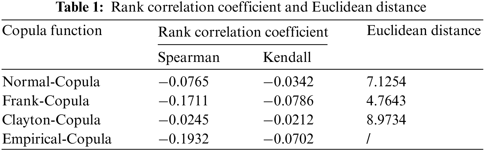
According to the Table 1, the rank correlation coefficient of the Frank-Copula function is close and the Euclidean distance between them is small, so the Frank-Copula function is selected to describe the correlation of wind and solar power output.

3.2 Scenario Generation and Reduction

First, the Gaussian kernel function based on the non-parametric kernel density estimation is used to generate the probability density function (PDF) of the wind and solar power outputs in each hour per day. Then, the optimized Frank-Copula function is adopted to establish the joint probability distribution function (JPDF) of the wind and solar power outputs in each hour. The JPDF is then sampled and the inverse transformation of Frank-Copula is performed on sampled data of the JPDF to obtain the sampling data of the wind and solar power outputs in each hour. It is difficult to solve the inverse function of its cumulative distribution function (CDF) because the PDF of the non-parametric kernel density estimation is a summation form. Therefore, the cubic spline interpolation method is used to solve the sampling values corresponding to its cumulative probability.

In summary, the steps of the scenario generation with considerations of the uncertainties and correlativity of wind and solar power outputs are as the following:

(1) After getting the historical n-day wind and solar power output (1 point per hour), the Gaussian kernel function is selected based on the non-parametric nuclear density estimation method to generate the wind and solar power output probability density function [23] for each period within 24 h.

fm,t(xt)=1nm∑d=1nK(xt−Xd,tm)(1)

fm,t(yt)=1nm∑d=1nK(yt−Yd,tm)(2)

where t = 1, 2,…, 24, represents the 24 time periods. In period t, the xt and yt are the wind and solar power outputs, respectively; the Xd,t and Ydt are the wind and solar power outputs during the t-time period of the day d; the m is window wide; the K(•) means a Gaussian kernel function, which expressed as:

K(xt−Xdtm)=(12π)exp⁡[−(xt−Xdt)22m2](3)

(2) According to the probability density function of the wind and solar power output in each period, the cumulative distribution function is found, then the joint probability distribution function of the wind and solar power output is established according to the Frank-Copula function, which is specifically expressed as follows:

F^(xt,yt)=C(F^xt(xt),F^yt(yt))(4)

C(ut,vt;λt)=−1λtln⁡(1+(e−λtut−1)(e−λtvt−1)e−λt−1)(5)

where the C represents the two-dimensional Frank-Copula function; the F^xt(xt) and F^yt(yt) represent the cumulative distribution function of the wind and solar power output, respectively; the ut and vt, are the same value as the F^xt(xt) and F^yt(yt). The λt is the correlation parameter. When λt ∈ (−1, 1) and λt ≠ 0, λt → 0, ut and vt have better independence; when λt > 0, ut is positively correlated with vt, when λt < 0, ut is negatively correlated with vt.

(3) The joint distribution function of each period was sampled, and the sampling wind and solar power output of each period with the cumulative probability was solved by the Cubic Spline Interpolation method.

Set a small interval:

{A=[(F^Xdt)−1(u),(F^Xd+1t)−1(u)]B=[(F^Ydt)−1(v),(F^Yd+1t)−1(v)](6)

Breaking the cumulative probability interval [0, 1] into d − 1 small intervals, in any interval A and B, with the cumulative probabilities u and v as the independent variables and x and y as the dependent variables, the Cubic polynomials on the interval are obtained as:

{x=(F^Xdt)−1(u)=adu3+bdu2+cdu+ldy=(F^Ydt)−1(v)=a′v3+b′v2+c′v+l′(7)

where the d = 1, 2,…, n, f = 1, 2,…, F, and the F is the sampling size. For any sampling cumulative probability values u(t)f and v(t)f, it must fall in an interval A and interval B, and substitute u(t)f and v(t)f into the upper Eq. (7) to find the sampling wind and solar power output for each period.

(4) Considering the large sampling size, in order to balance the calculation speed and accuracy, the K-means [24] clustering is used to cluster the annual photovoltaic and wind turbine power output data to obtain the typical daily data and to calculate the probability of each scenario with consideration of the calculation speed and accuracy. The specific steps are described in the literature [24].

4  Microgrid Deterministic Model Considering Multiple Scenarios

4.1 Structure of the MG

The MG consists primarily of a wind turbine (WT), a photovoltaic (PV), a combined heating and power (CHP), an electric boiler (EB), battery storage (BT), and heat storage (HS). The inputs of the MG are connected to the power grid. The electricity can be bought or sold to the power distribution system. The direction of the arrows in Fig. 2 indicates the direction of energy flow. The scheduling objective of MG is to minimize the total system cost and ensure a reliable energy supply considering uncertainties and certain constraints. The structure of the Microgrid and the framework flowchart of the proposed method is illustrated in Fig. 2.

Figure 2: Structure schematic of the MG

4.2 Objective Function

In this paper, we use the box decomposition algorithm [25] to decompose the variables into a two-stage solution model to minimize the total cost C, where the first stage considers the unit start-up and stop-down to determine the start-up and shut-down costs Cmp; the second stage considers the total cost Cope in MG operation in different scenarios. As shown in Eqs. (8)–(12):

minC=Cmp+Cope(8)

Cmp=cmp∑s=1Ns∑t=123γs,t(9)

Cope=∑s=1NspsCope,s(10)

where the cmp is the start-up and shut-down costs coefficient of the micro gas turbine; the γs,t is the linearized state variable of unit start-up and stop-down. The Cope,s is the total operating cost of the system under each scenario s. The Ns is a set of all scenarios, taken as 4; and the ps is the probability of scenarios s occurring.

Cope,s=∑t=1T[Cgrid,s,t+CG,s,t+CBT,s,t+Cqw,s,t+Cqv,s,t+CDR,s,t](11)

{Cgrid,s,t=cgrid,tbuyPs,tbuy−cgrid,tsellPs,tsellCG,s,t=cGPs,tGCBT,s,t=cBT(PBT,s,tch+PBT,s,tdis)Cqw,s,t=cqw(Ps,tpre−w−Ps,tw)Cqv,s,t=cqv(Ps,tpre−v−Ps,tv)CDR,s,t=cILPs,tIL+cCLPs,tSL+cCHLPs,tCHL(12)

where the T is the number of periods in the day, taken as 24. Eq. (11) indicates the total expression for the operation cost. Eq. (12) indicates the specific system operation cost, including the interaction cost with the distribution network Cgrid,s,t; micro gas turbine operation cost CG,s,t; battery aging cost CBT,s,t; wind and solar curtailment cost Cqw,s,t, Cqv,s,t; and demand response load compensation CDR,s,t.

4.3 Constraints

The above objective function is subject to the following constraints:

4.3.1 CHP Gas Turbine Unit Constraints

{ 0≤Ps,tG≤PmaxG−PmaxG(1−us,tG)−rd≤Ps,tG−Ps,t−1G≤PmaxG(1−us,tG)+ru(13)

0≤γs,t≤us,tGus,tG+us,t+1G−1≤γs,t≤us,t+1G(14)

where Eq. (13) is the upper and lower limit of the gas turbine output and the ramping constraint of the CHP unit and Eq. (14) is unit operating status constraint. The PmaxG is the maximum power of the micro gas turbine; the rd and ru respectively indicate the upward and downward climbing rate. The us,tG represents the status variable of the micro gas turbine under the scenario s, 1 represents the gas turbine operation, and 0 represents the shutdown.

4.3.2 Interaction with the Distribution Network Constraints

{0≤Ps,tbuy≤us,tgridPmaxgrid0≤Ps,tsell≤(1−us,tgrid)Pmaxgrid(15)

where Eq. (15) indicates the power interaction constraint between MG and the distribution network. The Pmaxgrid is the interactive power upper limit of the connection line between the MG and the distribution network and the upper limit of the power sold to the MG; the us,tgird represents the status variable of MG power purchase or sale in t period under scenario s, and 1 represents power purchase from the grid, 0 represents power sale for the grid.

4.3.3 Energy Storage System Constraints

{0≤PBT,s,tch≤us,tBTPmaxe0≤PBT,s,tdis≤(1−us,tBT)Pmaxe(16)

ηchBT∑t=1TPBT,s,tch−1ηdisBT∑t=1TPBT,s,tdis=0(17)

{SOCs,t=[E(0)+ηchBT∑t′=1tPBT,s,t′ch−1ηdisBT∑t′=1tPBT,s,t′dis]/Ebat.maxSOCmin≤SOCs,t≤SOCmax(18)

where Eq. (16) represents the charging and discharge power constraints of energy storage. Eq. (17) indicates that the capacity of battery storage is equal at the beginning and end of the scheduling, which is conducive to the cycle scheduling of battery storage. Eq. (18) represents the State of Charge (SOC) constraint. The us,tBT represents the charging and discharge state variable of the battery storage system in t period under scenario s, where 1 represents charging and 0 represents discharge; the Pmaxe represents the maximum charge and discharge power allowed for battery storage. The ηBTch and ηBTdis represent the power efficiency of the battery. The SOCs,t is the charge state of the battery in the t period under scenarios s, the SOCmax and SOCmin are the upper and lower limits of the charge state of the battery, respectively; the E(0) and Ebat.max are the initial and maximum capacity of battery storage.

4.3.4 Heat Storage System Constraints

{0≤PHS,s,tch≤us,tHSPmaxh0≤PHS,s,tdis≤(1−us,tHS)Pmaxh(19)

0.1sh≤ηHSch∑t=1TPHS,s,tch−1ηHSdis∑t=1TPHS,s,tdis+0.5sh≤0.9sh(20)

where Eq. (19) indicates the charging and discharge power constraints of the heat storage. Eq. (20) indicates the heat storage capacity constraint. The PHS,s,tch and PHS,s,tdis are respectively the heat storage charge and discharge heat power in the t period under the scenarios s. The us,tHS represents the energy release state variable of the heat storage system in t under scenarios s, where 1 represents energy and 0 represents energy release. The Pmaxh represents the maximum energy charging power allowed for heat storage; the ηHSch, and ηHSdis are the efficiencies of charging and discharging the energy of the heat storage system, respectively. The sh is rated capacity of heat storage equipment and taken as 300 kW.

4.3.5 Energy Balance Constraints

{PBT,s,tdis−PBT,s,tch+Ps,tbuy−Ps,tsell+Ps,tG+Ps,tv+Ps,tw=PtL+Ps,tDR+Ps,tEBPs,tDR=Ps,tIL+Ps,tSLPs,tEB≥0(21)

PBT,s,tdis−PBT,s,tch+λPs,tG+ξPtEB=PtHL−PtHCL(22)

where Eq. (21) represents the electric power balance constraint. Eq. (22) indicates the thermal power balance constraint. The Ps,tEB represents the electric power consumed by the electric boiler in period t under scenarios s, the Ps,tDR represents the demand response power in period t under scenarios s. The PtL represents the electric power and conventional electric load value consumed by the electric boiler in period t. The λ, ξ represent the thermal conversion efficiency of micro gas turbine and electric boiler, the PtHL indicates the conventional heat load.

4.3.6 Demand Response Load Constraints

{−αPtL≤PtSL≤αPtL0≤PtIL≤αPtL0≤PtHCL≤βPtHL∑t=1TPtdz=0(23)

where the α and β are the load adjustment range of interruptible electric load and reducing heat load, respectively, which are both taken as 0.1.

4.3.7 Scenario Constraints

∑s=1Nsps=1(24)

where Eq. (24) represents the sum of the probabilities in all scenarios s is 100%.

4.3.8 Wind and Solar Power Output Constraints

{0≤Ps,tw≤Pmaxw0≤Ps,tv≤Pmaxv(25)

where Eq. (25) represents the wind and photovoltaic power output constraints. The Ps,tw and Ps,tv are the actual output of wind and solar power at time t under scenario s, respectively. The Pmaxw and Pmaxv indicate the maximum output of wind power and photovoltaic, taken as 1000 and 200 kW, respectively.

5  Distributional Robust Optimization Model

5.1 Model Building

The deterministic model in multiple scenarios constituted by Eqs. (8)–(25) can be represented in the matrix form as:

miny,zs∈Zs(aTy+∑s=1NspsbTzs)(26)

{Ay≤fBzs≤xXy+Hzs=q(27)

where the y is the first stage variable, including various investment schemes in the MG; the a is the corresponding cost coefficient of y and b is the quadratic and primary cost coefficient in the objective function. The ps is the probability of occurrence of scenario s. The zs is the second stage variable under scenario s, the zs is the set of second stage variables under scenario s as: zs ∈ {Ps,tbuy, Ps,tsell, Ps,tG, PBT,s,tch, PBT,s,tdis, PtEB, Ps,tw, Ps,tv}. A, B, X, H, f, x, q, represent the matrix or vector corresponding to the variable in the model constraints. Eq. (27) respectively represents all constraints related to variables in the first stage; all constraints associated with the second stage variables; and all constraints on the association of the first stage variables with the second stage variables.

The uncertainty and correlation of wind and solar power output, as well as the limitations of historical data, and the scene probability distribution obtained by scene clustering have certain errors. To solve this problem, this paper uses stochastic programming to get the scene set, then uses a robust optimization method to limit the probability distribution of the scene.

By using the method of 3.2, we can first get a series of wind and solar power output scenarios considering their correlation, then the K-means reduction method can be used to obtain the original distribution probability ps0 of the reduced N original scenes and scene s. Finally, based on the 1-norm and ∞-norm confidence intervals to restrain the fluctuation range of the probability distribution, a DRO is constructed. The constraints of DRO can be the same as the deterministic model, i.e., Eqs. (14)–(25), and the objective function is:

minymax{ps}∈Ωpminzs∈Zs(aTy+∑s=1NspsbTzs)(28)

where the Ωp is the set interval of the probability distribution of the scenarios, representing the confidence set [26] set by the 1-norm and ∞-norm constraints.

The confidence degree of the probability distribution p can be expressed as:

pr(‖p−p0‖1≤θ1)≥1−2Nsexp⁡(−2Nθ∞Ns)(29)

pr(‖p−p0‖∞≤θ∞)≥1−2Nsexp⁡(−2Nθ∞)(30)

where the pr(•) is the probability solver function; the p0 is the predicted value of the probability distribution; the θ1 and θ∞ are the allowable deviation values of the probability distribution. For the right side of the above 2 inequalities: the 1 − 2Ns exp(−2Nθ1/Ns) and 1 − 2Ns exp(−2Nθ∞), set them to α1 and α∞, respectively, N is number of original scenes, taken as 1000. Then the α1 and α∞ denote the confidence levels satisfied by the probability distribution p based on 1-norm and ∞-norm confidence, respectively. The θ1 and θ∞ can be expressed as:

θ1=Ns2Nln⁡2Ns1−α1(31)

θ∞=12Nln⁡2Ns1−α∞(32)

Based on this, the confidence set of the probability distribution can be deduced as:

Ωp{ { ps }|ps≥0,s=1,…,Ns∑s=1Nsps=1∑s=1Ns| ps−ps0 |≤θ1max1≤s≤Ns| ps−ps0 |≤θ∞(33)

5.2 Model Solution

The model constructed in this paper is a multi-stage optimization problem that cannot be solved directly by commercial solvers. Using the column constraint generation algorithm (C&CG) [27] to solve. Similar to the Benders decomposition algorithm, the C&CG algorithm also obtains the optimal solution of the original problem by decomposing the original problem into a master problem and a sub problem for alternate solutions. The difference between the two is that the C&CG algorithm continuously introduces variables and constraints related to the sub problem in the process of solving the master problem, which can obtain a more compact lower bound on the value of the original objective function and thus effectively reduce the number of iterations.

5.2.1 Master Problem

The objective of the master problem is to solve for the optimal solution that satisfies the economy of the system given the known probability distribution p of the scenario, which can be expressed as:

LM=miny,γ,zs∈Zs(aTy+γ)(34)

γ≥∑s=1Nsps(n)∗(bTzs(n))n=1,2,…N(35)

where the superscript “*” denotes the optimal solution for the corresponding variable; the γ is the given threshold, and the N is the total number of model iterations. The variables y∗ and the lower bound LM of the model can be obtained by solving the master problem.

5.2.2 Sub Problem

The sub problem is a two-layer structure of max-min form, which can be expressed as:

fsp(y∗)=max{ps}∈Ωpminzs∈Zs∑s=1Nsps(bTzs)(36)

where Eq. (36) is to assume that the variable zs can be flexibly adjusted according to the scene change adjustment. When the result of solving the master problem is known to be y∗. The lower bound value of the model Eq. (28) is solved by finding the worst-case scenario probability distribution within the confidence interval.

1 hown:

hs=minzs∈Zs(bTzs)(37)

U=max{ps}∈Ωp∑s=1Nspshs(38)

where the hs represents the solution to the inner layer problem and can be obtained from the result of solving the master problem. The U represents the solution to the inner layer problem after the value of hs is known. Since the absolute value constraint in Eq. (33) is a nonlinear constraint, a linear equivalent decomposition is required.

The equivalent transformation of the absolute value constraint is obtained as:

{∑s=1Ns(ps++ps−)≤θ1ps++ps−≤θ∞μs++μs−≤1ps+≤μs+θ1ps−≤μs−θ1ps=ps0+ps++ps−∀s(39)

where ps+ and ps− are the positive and negative offsets of the probability distribution ps of the scenario s with respect to ps0, respectively; the μs+ and μs− are the 0–1 variables that produce positive and negative offset to the ps, respectively.

5.2.3 Model Solving Steps

After the above steps, the model is transformed into a mixed linear planning problem, which can be solved directly by the commercial solver to get the ps∗. By substituting the master problem for the next iteration optimization, the upper limit UM of the model can be obtained. The specific solution process is as follows:

Step1: set the lower bound LM = ∞ and the upper bound UM = ∞, set the iteration time n = 1;

Step2: solve master problem, obtain the optimal solution (y*, γ*), update the lower bound value to LM = min(aTy*+ γ*);

Step3: fix the first stage variable y* constant, solve the sub problem to obtain the worst-case probability value ps∗ and the objective function value fsp(y*), update the upper bound to UM = min{UM, aTy*+ fsp(y*)};

Step4: stop the iteration and return the optimal solution y* if UM − LM < ϵ, otherwise, update the worst-case probability distribution of the master problem psn+1 = ps∗, then add new constraints related to the new variable zsn+1 to the master problem;

Step5: update the number of iterations, n = n + 1, and return to Step2.

6  Example Analysis

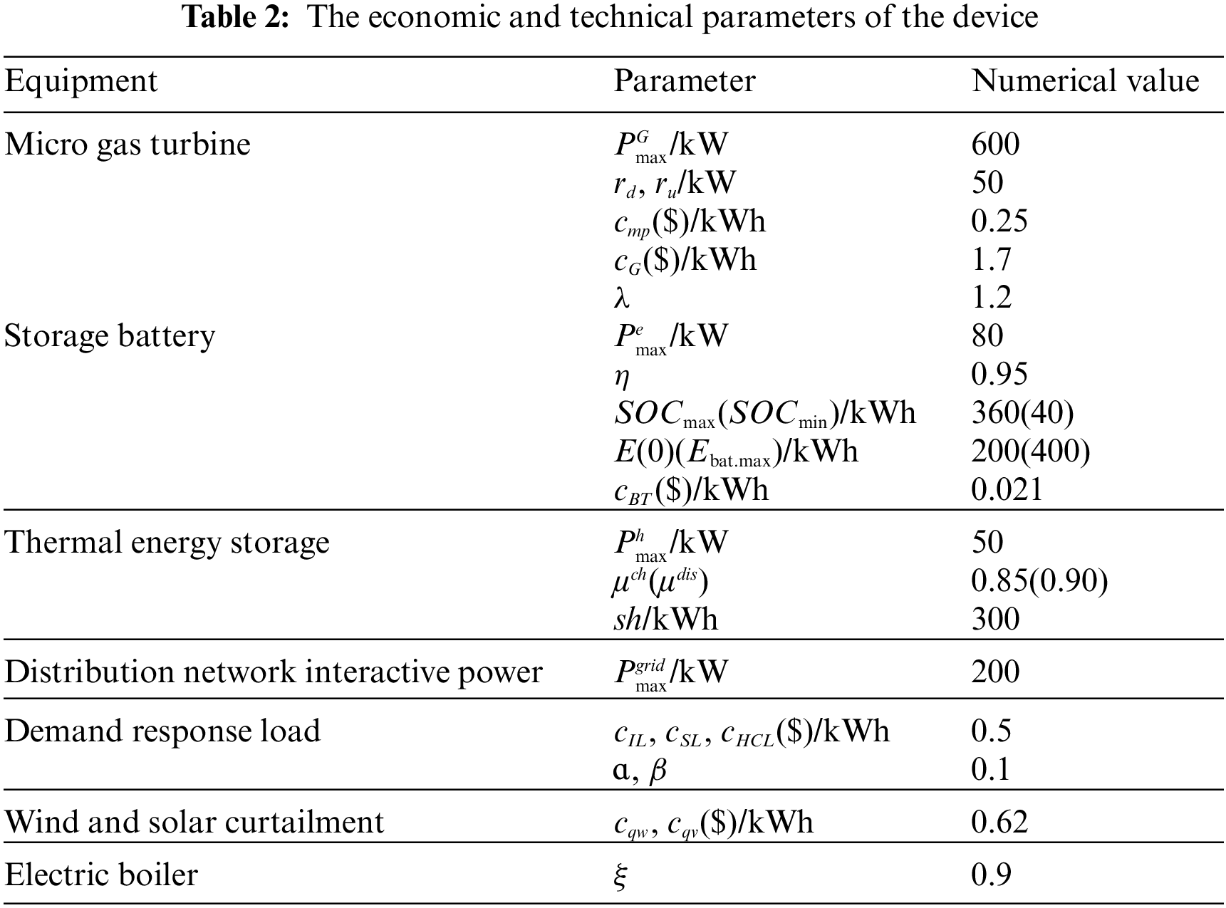
This paper follows the MG as shown in Fig. 1 tos verify the effectiveness of the two-stage DRO model and the solution algorithm proposed there. See Fig. 2 for the purchase and sale of electricity prices interacting with the power grid. Based on a 2017 study of a microgrid system in a location in Jiangsu Province, China, data related to wind turbines, photovoltaic power stations, micro gas turbines, electric boilers, energy storage, and thermal storage were obtained. The details are shown in Table 2. The model in this paper is based on the Matlab R2020b platform and has been optimally solved using the YALMIP/CPLEX solver.

The C&CG algorithm was solved iteratively in stages using the algorithm presented in Section 5, with a computational time of 6.436516 s. The power price for buying and selling between microgrid system and power grid are shown in Fig. 3. The iteration results are shown in Fig. 4, showing that the optimal value can be obtained after the second iteration, and the operation rate is very fast.

Figure 3: Power price for buying and selling between microgrid system and power grid

Figure 4: C&CG algorithm iteration results

6.1 Scenarios Generation Analysis

Based on 3.2, we can obtain some scenarios based on the Frank-Copula function to consider the wind and solar power correlation output. The sampling scale F is taken as 1000 and the results are shown in Appendix B1. Then the K-means clustering is used to reduce the scenarios, and obtain 4 sets of typical wind power and photovoltaic output curves, as shown in Fig. 4. The probability of each scenario was 0.26, 0.29, 0.15, and 0.30.

As can be seen from Fig. 5, the changes in wind and solar power output are consistent or opposite in certain time periods, showing some correlation in the following scenarios. It shows that the scenario reduction results reflect the uncertainty and correlation between wind and solar power output. The wind and solar power characteristics of the region can be simulated well, which is conducive to the overall optimization and operation of the system.

Figure 5: The scenario reduction results of WT and PV output

6.2 Scenarios Generation Analysis

6.2.1 Interpretation of Result

This section mainly analyzes the impact of adding demand response to a microgrid system containing the energy storage, the heat storage, and the micro gas turbines on system optimization. The scheduling results in other scenarios are shown in Appendix B2 Figs. B2–B4.

Figure B3: Demand response load transfer and electric/heat power balance in scenario 3

Figure B4: Demand response load transfer and electric/heat power balance in scenario 4

According to Figs. 6 and 7, comparing the electrical/heat load curve before and after IDR, we can find: the peak-valley difference of electric load decreased from 382.215 to 268.314 kW and thermal load from 291.652 to 262.487 kW. It can be seen that the participation of IDR in the system operation can effectively reduce the peak power/heat load, which makes the various load curves milder, and help to smooth the system operation.

Figure 6: The demand response load transfer situation in scenario 1

Figure 7: The electrical and heat balance situation in scenario 1

During the 24:00 to 8:00 period, the photovoltaic does not work and the wind power output is relatively small. Considering the start-up and shut-down costs of the gas turbine, the heat preparation is not started. At this time, the power shortage of the electric load is obtained by purchasing power from the external power grid, and the heat load is met by the heating of the electric boiler, due to low electricity prices, the battery storage system starts charging.

During the 8:00–14:00 periods, the photovoltaic starts to supply power, the battery storage system discharges; and sells electricity to the grid during the rich periods to make profits, and the micro gas turbine starts to meet the power supply pressure during peak electric load. At the same time, the energy storage and the heat storage system are discharged.

During the 14:00–18:00 period, as the load pressure decreases, photovoltaic and wind power can be used to meet the power supply demand, the micro gas turbine is shut down, and the MG sells electricity to the power grid, and the excess power is sold to the grid as much as possible, and then stored by energy storage, and the heat of the electric boiler is stored by the heat storage system.

From 18:00 to 20:00, with the peak of the electric heat load coming again, the micro gas turbine starts again, and the energy storage and heat storage system respectively discharge the heat. Then from 20:00 to 24:00, the photovoltaic stops working; due to the low electric thermal load supply pressure at this time, the micro gas turbine is stopped by the wind power and electric boiler, charges the energy storage system, and sells electricity to the grid when the power is rich.

To sum up, after the introduction of IDR and the configuration of the energy storage system, the electric thermal load is reduced, and the operation mode of the energy storage device is in line with the strategy of “low charge and high discharge”, which is more conducive to reducing the cost of microgrid energy purchase.

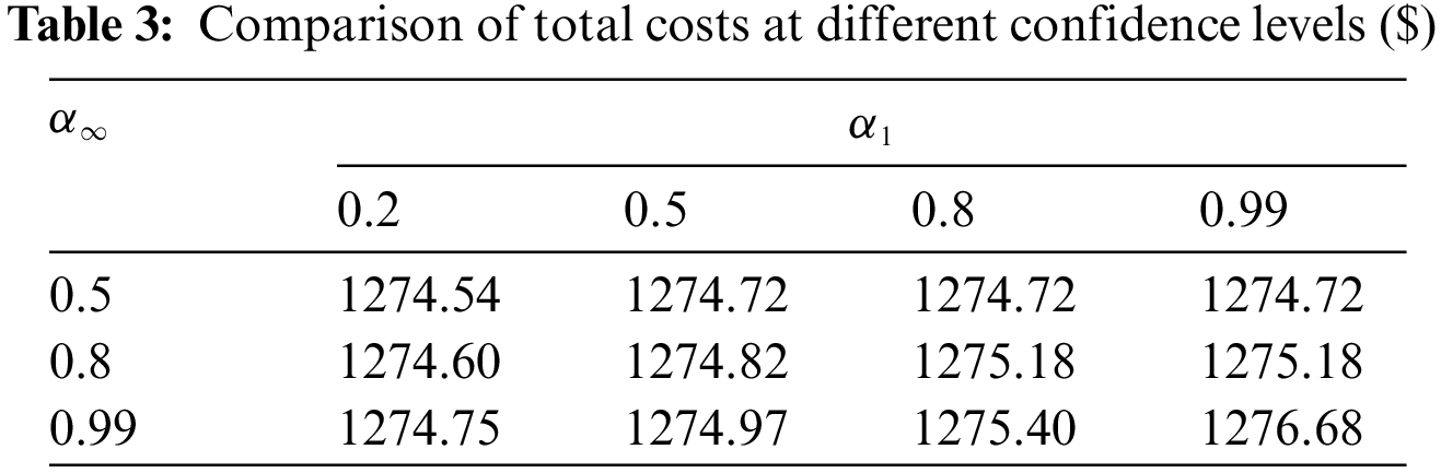
6.2.2 Cost Analysis with Different Confidence Intervals and Norms

Different confidence intervals were set to calculate the total cost of the model separately, and the results are shown in Table 3. It can be seen that when the values of α1 and α∞ are larger, the confidence interval is larger and the range of the corresponding uncertainty probability distribution is larger, which leads to a higher total cost for the system. However, when the value of α1 is small, the total system cost does not increase as α1 increases, indicating that the optimization results at this time are mainly affected by the ∞-norm.

The cost of each scenario obtained from the scenarios analysis method is taken as the known condition. The DRO model is operated under the conditions of the comprehensive norm, only 1-norm, and only ∞-norm respectively, and the corresponding costs are shown in Tables 4 and 5. When considering only 1-norm, let α1 = 0.5, 0.5 ≤ α∞ ≤ 0.99, and when considering only ∞-norm, let α∞ = 0.99, 0.2 ≤ α1 ≤ 0.99. As shown in Tables 4 and 5, the system is more conservative and the total cost is higher when only the 1-norm or only the ∞-norm is considered. It indicates that the selected and considered integrated norm scenario constraints has better economy.

6.2.3 Comparison of Results with Other Traditional Methods

The decision results of the DRO model are analyzed in comparison with those of the traditional stochastic optimization and robust models. The optimization results obtained by the two methods are compared by generating 1000 scenes in random simulation. where the values of α1 and α∞ are both taken as 0.99 in the DRO method. A stochastic programming approach for optimal scheduling with a probability of 0.25 for each scenario. The robust optimization methods are performed according to the [12]. Each of the above methods is performed under the same equipment configuration conditions.

The results are shown in Table 6.

According to the results, it can be seen that the robust optimization model corresponds to the worst clean energy consumption rate and profit; and the stochastic programming corresponds to the optimization results with the best economy and the best clean energy consumption rate, but conservation is not guaranteed. Compared with robust optimization and stochastic programming, the DRO method can achieve a better balance of economy and conservativeness, maximize the profitability of the distribution network while improving the consumption rate of clean energy, and has more advantages in dealing with uncertainty optimization.

7  Conclusion

Firstly, based on the stochastic optimization model, the output correlation between wind power and photovoltaic is analyzed. Secondly, based on the nonparametric nuclear density estimation and Frank-Copula function, a typical sample of 1000 sets of wind and solar power output with correlation was generated, and the reduced scenario is obtained through K-means clustering. Finally, we constructed the distributed robust optimization model that considers the confidence interval of a probability distribution. After simulation verification and comparison, indicates that our model can well balance system economy and robustness. The following conclusions can be drawn:

(1) The method of scenario generation has an important impact on the overall optimization results. The Frank-Copula function is used for scenario generation, which can better reflect the wind power and PV output correlation. Combined with the K-means scenario clustering algorithm for scenario reduction, the final generated scenarios can be more representative.

(2) The simulation results show that the participation of demand response reduces the peak-to-valley difference of the overall load. Rather than considering only 1-norm and ∞-norm, the combined norm reduces costs.

(3) By considering the confidence interval of the probability distribution based on the stochastic optimization model, the proposed DRO model in this paper can achieve a better balance of economy and conservativeness. Compared to stochastic programming and robust optimization, this method has more advantages in dealing with uncertainty optimization.

(4) C&CG algorithm can effectively and quickly solve the proposed distribution robust optimization model.

Acknowledgement: We would like to thank the editorial and reviewer panel for their input and comments.

Funding Statement: This work was supported in part by the National Natural Science Foundation of China (51977127); in part by the Shanghai Municipal Science and in part by the Technology Commission (19020500800), “Shuguang Program” (20SG52) Shanghai Education Development Foundation and Shanghai Municipal Education Commission.

Conflicts of Interest: The authors declare that they have no conflicts of interest to report regarding the present study.

References

1. Li, H., Lü, M., Hu, L. (2019). Review of CIRED, 2017 on microgrid planning and operation. Power System Technology, 43(4), 1465–1471 (in Chinese). [Google Scholar]

2. Zhai, H., Yang, M., Zhao, L. (2019). Three-phase robust dynamic reconfiguration of the distribution network to improve acceptance ability of distributed generator. Automation of Electric Power Systems, 43(18), 35–47 (in Chinese). [Google Scholar]

3. Chen, H., Tang, Z., Lu, J. (2021). Research on optimal dispatch of a microgrid based on CVaR quantitative uncertainty. Power System Protection and Control, 49(5), 105–115 (in Chinese). [Google Scholar]

4. Wang, M., Yu, H., Lin, X., Jing, R., He, F. et al. (2020). Comparing stochastic programming with posteriori approach for multi-objective optimization of distributed energy systems under uncertainty. Energy, 210, 118571. https://doi.org/10.1016/j.energy.2020.118571 [Google Scholar] [CrossRef]

5. Alabi, T. M., Lu, L., Yang, Z. (2021a). A novel multi-objective stochastic risk co-optimization model of a zero-carbon multi-energy system (ZCMES) incorporating energy storage aging model and integrated demand response. Energy, 226(C), 120258. https://doi.org/10.1016/j.energy.2021.120258 [Google Scholar] [CrossRef]

6. Yu, D., Yang, M., Zhai, H. (2016). An overview of robust optimization used for power system dispatch and decision-making. Automation of Electric Power Systems, 40(7), 134–143 (in Chinese). [Google Scholar]

7. Liu, X., Li, Y., Shi, Y., Shen, Y. (2022). Distributionally robust optimization model of virtual power plant considering user participation uncertainty. Electric Power Automation Equipment, 42(7), 84–93 (in Chinese). [Google Scholar]

8. Cao, J., Zeng, J., Liu, J., Xue, F. (2022). Distributionally robust optimization method for grid-connected microgrid considering extreme scenarios. Automation of Electric Power Systems, 46(7), 50–59 (in Chinese). [Google Scholar]

9. Liu, H., Qiu, J., Zhao, J. (2022). A data-driven scheduling model of virtual power plant using Wasserstein distributionally robust optimization. International Journal of Electrical Power and Energy Systems, 137(2), 107801. https://doi.org/10.1016/j.ijepes.2021.107801 [Google Scholar] [CrossRef]

10. Wei, Z., Guo, Y., Wei, P., Huang, Y., Fang, T. (2021). Distribution robust expansion planning model for integrated natural gas and electric power systems considering transmission switching. Electric Power Automation Equipment, 41(2), 16–23. 202012016 (in Chinese). [Google Scholar]

11. Ma, X., Guo, X., Lei, J. (2018). Capacity planning method of distributed PV and P2G in the multi-energy coupled system. Automation of Electric Power Systems, 42(4), 55–63 (in Chinese). [Google Scholar]

12. Liu, Y., Guo, L., Wang, C. (2018). Economic dispatch of microgrid based on two-stage robust optimization. Proceedings of the CSEE, 38, 4013–4022+4307 (in Chinese). [Google Scholar]

13. Siqin, Z., Niu, D., Wang, X., Zhen, H., Li, M. et al. (2022). A two-stage distributionally robust optimization model for P2G-CCHP microgrid considering uncertainty and carbon emission. Energy, 260(1), 124796. https://doi.org/10.1016/j.energy.2022.124796 [Google Scholar] [CrossRef]

14. Georgios, M., Kristina, O., Jan, C. (2018). Uncertainty and global sensitivity analysis for the optimal design of distributed energy systems. Applied Energy, 214, 219–238. https://doi.org/10.1016/j.apenergy.2018.01.062 [Google Scholar] [CrossRef]

15. Qiu, H., Long, H., Gu, W., Pan, G. (2021). Recourse-cost constrained robust optimization for microgrid dispatch with correlated uncertainties. IEEE Transactions on Industrial Electronics, 68(3), 2266–2278. https://doi.org/10.1109/TIE.2020.2970678 [Google Scholar] [CrossRef]

16. Yang, P., Shi, L., Ni, Y. (2017). Modeling of multiple wind farms output correlation based on copula theory. The Journal of Engineering, 13, 2303–2308. [Google Scholar]

17. Li, Z., Li, P., Yuan, Z., Xia, J., Tian, D. (2022). Optimized utilization of distributed renewable energies for island microgrid clusters considering solar-wind correlation. Electric Power Systems Research, 206(9), 107822. https://doi.org/10.1016/j.epsr.2022.107822 [Google Scholar] [CrossRef]

18. Luo, Y., Yang, D., Yin, Z., Zhou, B., Sun, Q. (2020). Optimal configuration of hybrid-energy microgrid considering the correlation and randomness of the wind power and photovoltaic power. IET Renewable Power Generation, 14(4), 616–627. https://doi.org/10.1049/iet-rpg.2019.0752 [Google Scholar] [CrossRef]

19. Jiang, Y., Chen, X., Fu, S. (2022). Day-ahead stochastic optimization method of microgrid considering the correlation of wind power. Journal of Global Energy Interconnection, 5(1), 46–54 (in Chinese). https://doi.org/10.19705.2022.01.006 [Google Scholar]

20. Papaefthymiou, G., Kurowicka, D. (2009). Using copulas for modeling stochastic dependence in power system uncertainty analysis. IEEE Transactions on Power Systems, 24(1), 40–49.https://doi.org/10.1109/TPWRS.2008.2004728 [Google Scholar] [CrossRef]

21. Wang, J., Cai, X., Ji, F. (2013). A simulation method of correlated random variables based on Copula. Proceedings of the CSEE, 33(22), 75–82 (in Chinese). [Google Scholar]

22. Zhou, S. (2016). Power system operation risk assessment considering wind-solar generation correlation based upon Copula theory. Guangzhou, China: South China University of Technology (in Chinese). [Google Scholar]

23. Huang, H., Zhou, M., Li, G. (2019). Coordinated decentralized dispatch of wind-power-integrated multi-area interconnected power systems considering multiple uncertainties and mutual reserve support. Power System Technology, 43(2), 381–389 (in Chinese). [Google Scholar]

24. Huang, W., Zhang, N., Yang, J., Wang, Y., Kang, C. (2019). Optimal configuration planning of multi-energy systems considering distributed renewable energy. IEEE Transactions on Smart Grid, 10(2), 1452–1464. https://doi.org/10.1109/TSG.2017.2767860 [Google Scholar] [CrossRef]

25. Cho, Y., Ishizaki, T., Ramdani, N. (2019). Box-based temporal decomposition of multi-period economic dispatch for two-stage robust unit commitment. IEEE Transactions on Power Systems, 34(4), 3109–3118. https://doi.org/10.1109/TPWRS.2019.2896349 [Google Scholar] [CrossRef]

26. Ruan, H., Gao, H., Liu, J. (2019). A distributionally robust reactive power optimization model for active distribution network considering reactive power support of DG and switch reconfiguration. Proceedings of the CSEE, 39(3), 685–695. [Google Scholar]

27. Zeng, B., Zhao, L. (2013). Solving two-stage robust optimization problems using a column-and-constraint generation method. Operations Research Letters, 41(5), 457–461. https://doi.org/10.1016/j.orl.2013.05.003 [Google Scholar] [CrossRef]

Appendix A1

Figure A1: The annual wind power and photovoltaic output in 2017 for testing area

Appendix A2

The specific mathematical expressions of the 5 common types of Copula functions are shown below:

(1) Normal-Copula:

C(u,v;ρ)=∫−∞Φ−1(u)∫−∞Φ−1(v)12π1−ρ2exp⁡(−s2−2ρst+t22(1−ρ2))dsdt(A1)

where −1≤ρ≤1 is the dependence parameter, Φ and Φ−1 are the standard normal distribution and its inverse function, respectively.

Multidimensional Normal-Copula:

C(u1,u2,…,un;ρ)=Φρ(Φ−1(u1),Φ−1(u2),…,Φ−1(un))(A2)

where ρ is the equivalent correlation matrix, Φ and Φ−1 are the standard normal distribution and it is inverse function.

(2) Frank-Copula:

CF(u,v;θ)=−θ−1log⁡(1−(1−e−θu)(1−e−θv)(1−e−θ))(A3)

where the dependence parameters θ≠0. When θ>0 indicates positive correlation, when θ→0 indicates mutual independence, when θ<0 indicates negative correlation.

(3) Clayton-Copula:

CCl(u,v;θ)=Max((u−θ+v−θ−1)−1θ,0)(A4)

where the dependence parameter θ∈[−1,+∞), and θ≠0.

The expressions of the probability density functions of the 5 common types of Copula functions are shown in Fig. A2.

Figure A2: Distribution density of three Copula functions

Appendix B1

Figure B1: Sampling results after applying the Copula function

Appendix B2

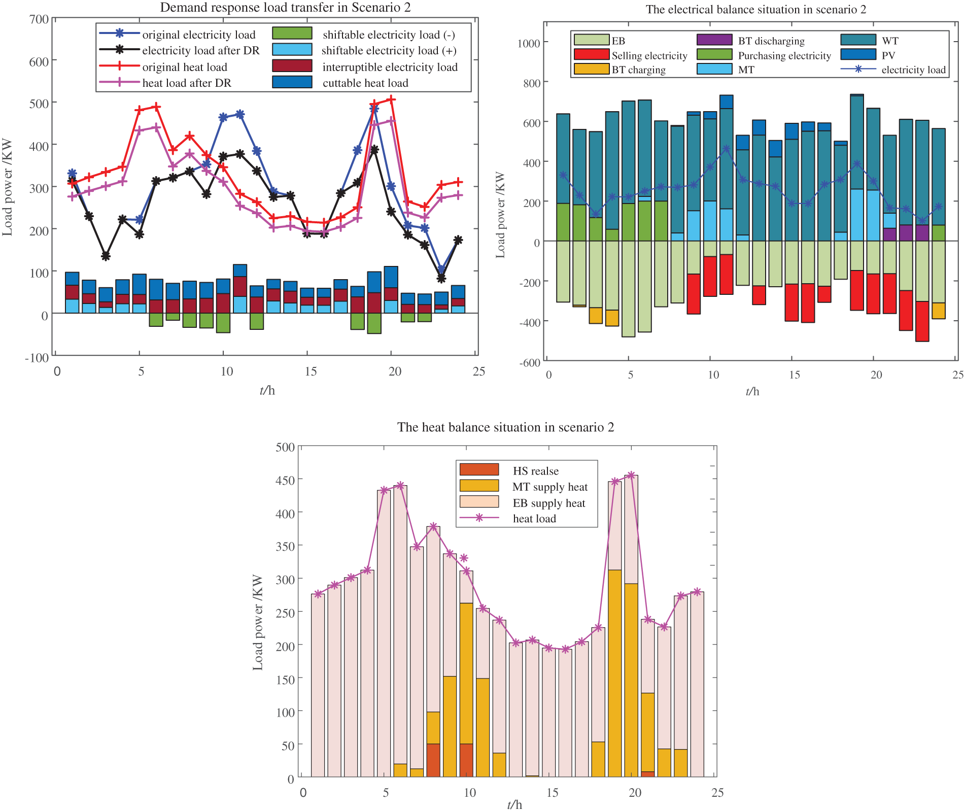
Figure B2: Demand response load transfer and electric/heat power balance in scenario 2