Distribution Line Longitudinal Protection Method Based on Virtual Measurement Current Restraint

Nomenclature

1  Introduction

Energy and the environment are major constraints on social development. The pressure on environmental protection has been growing since the Industrial Revolution. Against this background, energy conservation and emission reduction, sustainable development, and utilization of renewable energy have become the development strategies of countries around the world [1]. PV energy has a growing development trend as a representative of clean energy. The access of PVs changes the behavior and the characteristics of traditional distribution networks. A multi-source operation mode is formed and the uncertainty of power flow direction increases. Meanwhile, the PV system contains a large number of power electronic converter devices. The variety of control strategies changes the fault characteristics and affects the existing protection principles. It could reduce the reliability of existing protections and threaten the safety and stable operation of distribution networks [2,3]. Therefore, it is necessary to find a distribution network protection method that is suitable for PV interconnection to help the realization of the green and low-carbon energy transition.

In a traditional radial distribution network, the regular direction of power flow is from the power substation to various loads. The traditional overcurrent protection achieves coordination between each protection stage by adjusting the action time and setting values [4,5]. After the access of PVs, the distribution network changes from a single power supply to multiple power supplies. The distribution of power flow becomes uncertain. The fault current features of PVs are subject to multiple conditional nonlinear constraints such as voltage drop [6,7], which makes it difficult to update the setting value of the protection system. Traditional protection loses its original selectivity and reliability, which affects the safe and steady operation of the distribution network. These factors set limits to the development of PV connecting to the distribution network.

Differential protection adopts the measured difference from both terminals of protected zones. It has extremely strong selectivity and can operate swiftly if communication can respond in time. Combined with the fault current characteristics of PVs, the corresponding differential protection calculation setting methods are proposed. References [8,9] proposed a protection method based on the phase shift of positive sequence current collected by the protection devices on both sides after a fault occurs in the fault zone. References [10,11] proposed a protection method based on short-circuit current variation through the fault characteristics of forward and reverse fault phase variation. References [12,13] used Fourier transform for frequency deviation, current, and noise to accurately extract phase information, and discussed uncertain factors such as light intensity that affect the PV output to determine the range of phase shift. Chisava et al. [14] proposed a differential protection method based on the time-domain analysis of the voltage and current signals. To meet the data synchronization requirement of differential protection, some references also presented improved current differential protection methods [15–17] and other differential protection, such as impedance differential protection [18] and power differential protection [19]. However, these references do not address the uncertainty of PV output.

Therefore, it is important to propose a protection method with high reliability for the distribution network with PV access. This paper proposes a distribution line longitudinal protection method based on virtual measurement of current restraint. Firstly, the impact of PV connected to the distribution network on differential current protection is analyzed. Secondly, for the output of unmeasurable PVs, the equivalent compensation relationship is constructed by using the modified virtual compensation current to determine the degree of compensation, so as to adjust the measurement current adaptively. This method can compensate for the real-time output of PV and ensure accurate action of the protection devices. Next, an improved edit distance algorithm is proposed to compare the similarity between the actual model current and the virtual measurement current to discriminate internal and external faults. Finally, simulations are used to analyze the adaptability and denoising capability of the improved edit distance algorithm under different operating scenarios. Also, the performance of the proposed protection method is verified by a simulated model on the PSCAD platform.

2  Effect of PV on Current Differential Protection

2.1 Grid-Connected Equivalent Modeling of PV

The equivalent grid-connected topology of PV is shown in Fig. 1. PV batteries generate direct current, which is boosted through a DC-DC converter to realize maximum power point tracking (MPPT), and then it is connected to the grid through a DC-AC converter and a filter circuit.

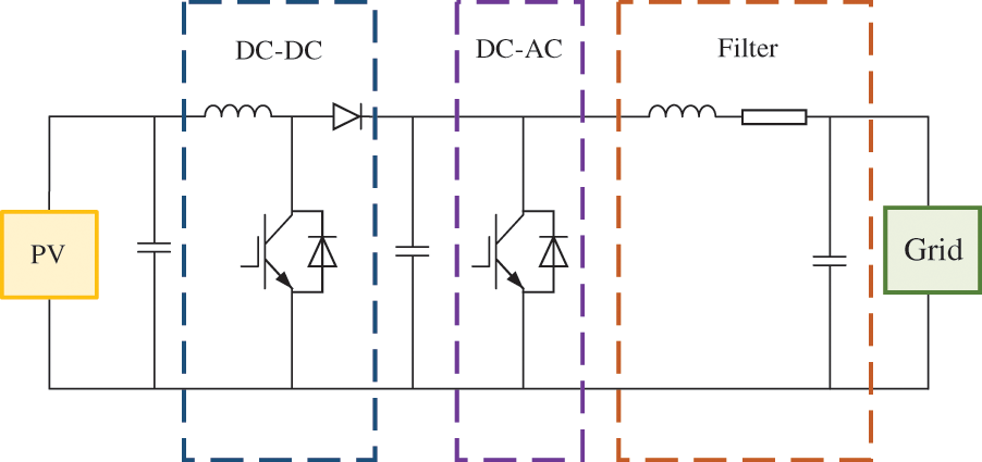
Figure 1: Grid-connected equivalent circuit

When a fault occurs, the PV must have the low voltage ride-through (LVRT) capability to meet the reactive power support requirements of the system due to the voltage drop at the fault point. When the voltage drops below 90%, the outer voltage loop of the controlling strategy is disconnected. During LVRT, the active and reactive current instructions are shown in Eq. (1).

{Id=IN,Iq=0(U1>0.9UN)Id=min{2P∗3Upcc,(KmaxIN)2−Iq2}(0.2UN<U1<0.9UN)Iq=1.5×(0.9−UpccUN)IN(0.2UN<U1<0.9UN)Id=0,Iq=KmaxIN(U1<0.2UN)(1)

The variables Id and Iq represent the active and reactive components of the PV output current, respectively. Kmax denotes the ratio between the maximum amplitude provided by PV and the normal operation current, and Kmax=1.2. Different equations are selected according to different voltage drop levels. For example, when voltage drops to a value higher than 0.9UN, only Id is provided and Iq is 0; when a short-circuit fault occurs and the voltage drops between 0.2UN and 0.9UN, the current Id and Iq are provided according to the control strategy as in Eq. (1), and so on. Since the transient process of PV equipment is fast and does not affect its steady-state output, the transient process of its internal control strategy switching can be ignored. PV was traditionally modeled by a rotating motor. However according to the fault output characteristics of PV during LVRT, it is better to model a PV with a voltage-controlled current source whose current is controlled by the voltage of the connection point. When a fault occurs, the equivalent circuit of PV connecting to the distribution network is shown in Fig. 2 and its specific output characteristics are shown in the output equation of Eq. (1).

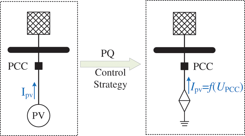
Figure 2: Equivalent circuit diagram of PV connecting to the grid

2.2 Current Differential Protection Setting

Current differential protection has spontaneous selectivity, which only reflects internal faults. Moreover, the differential current of internal faults is large, while the differential current is small under external faults and normal conditions. The protection principle is shown in Fig. 3.

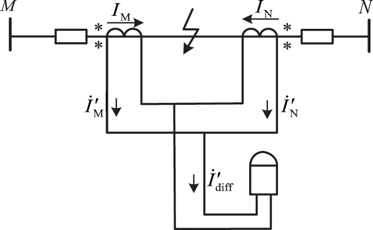
Figure 3: Schematic diagram of current differential protection

|I˙′M+I˙′N|>Iset(2)

|I˙′M+I˙′N|>krel⋅|I˙′M−I˙′N|(3)

Eqs. (2) and (3) form a differential criterion with percentage restraint. Iset indicates the minimum action current that should avoid the maximum unbalanced current under external faults and normal conditions. When Eqs. (2) and (3) are satisfied simultaneously, the protection will act.

As PVs are connected to the distribution network, the unbalanced current of current differential protection increases. The protection is difficult to operate reliably. Fig. 4 shows the different operating conditions of the distribution network with PV interconnection. The part inside the dotted line represents the protection zone.

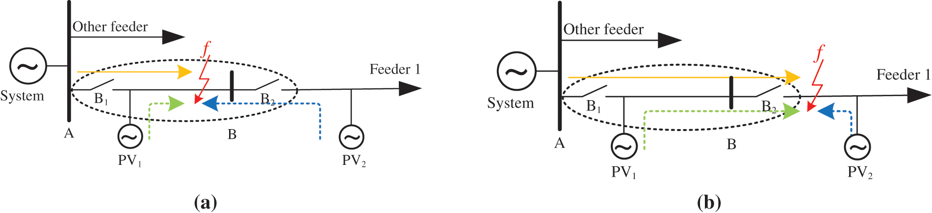
Figure 4: Impact of PV connection on current differential protection, (a) Schematic diagram of internal faults, (b) Schematic diagram of external faults

(1) When an internal fault occurs within the protection zone, as shown in Fig. 4a, the voltage within the protection area decreases and the feeding current of PVs increases. The PV2 plays a positive role in increasing the differential current value, while the impact of the PV1 on the current differential protection is manifested as a shunt effect.

To illustrate the effect of PVs within and beyond the protection zone, the changes of differential current are discussed when the capacity of only one PV varies. As shown in Fig. 5a, the capacity of internal PV1 keeps unchanged, but the capacity of external PV2 increases. The differential current which is marked by the blue line rises with the increase of the capacity of PV2. On the other hand, the capacity of external PV2 keeps 1 MW, and the capacity of internal PV1 increases. As shown in Fig. 5b, the differential current drops when the capacity of PV1 increases. The red dotted line indicates the differential current threshold Iset. From the two figures in Fig. 5, the differential currents are all larger than the protection threshold.

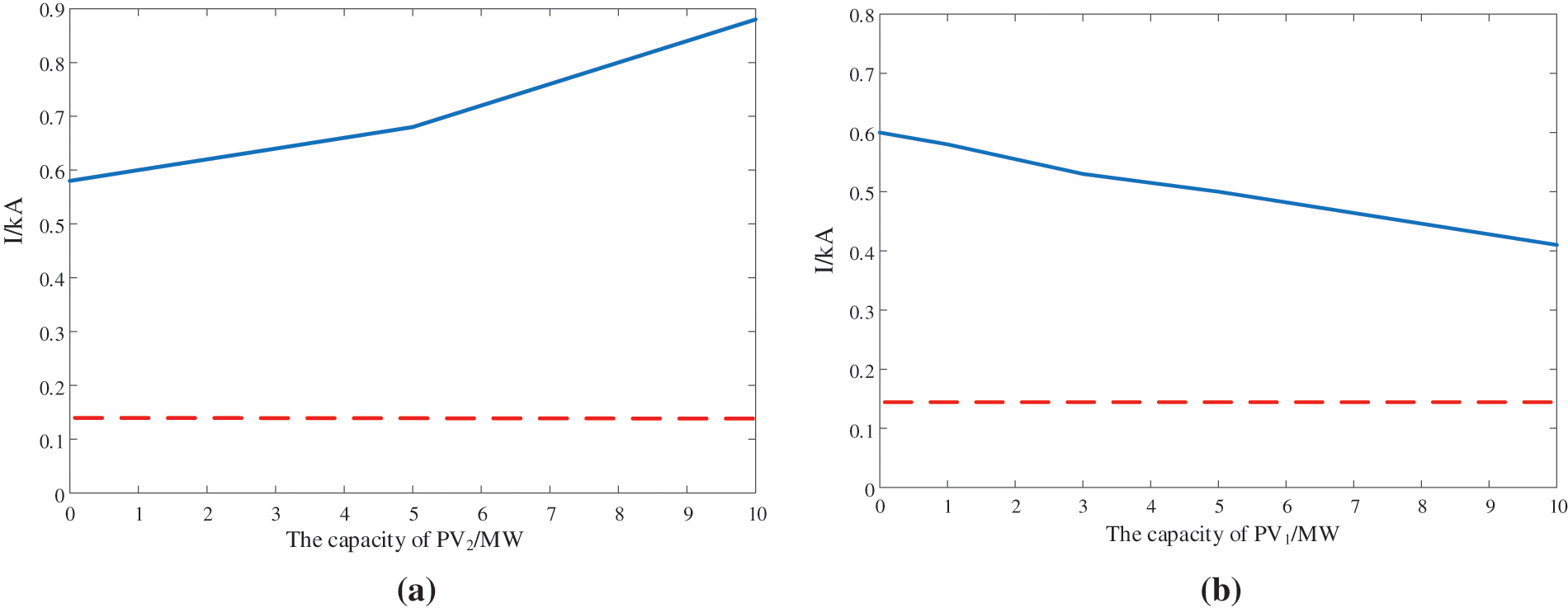
Figure 5: Impact of PV capacity on differential current when internal fault occurs, (a) The capacity of PV1 is 1 MW, and the capacity of PV2 varies from 1 to 10 MW, (b) The capacity of PV1 varies from 1 to 10 MW, and the capacity of PV2 is 1 MW

2) External fault f occurs downstream of the protection zone, as shown in Fig. 4b. As the PV1 within the protection zone will feed currents when an external fault occurs, the differential current of the protection zone will increase accordingly. As shown in Fig. 6, the differential current value changes with the PV capacity when an external fault occurs. To prevent the misoperation of current differential protection in case of external faults, the action current threshold should be larger.

Figure 6: Impact of PV capacity on the differential current of external fault

To eliminate the effect of feeding currents from internal PVs, the minimum action current Iset should meet the following relation as shown in Eq. (4).

Iset≥krel⋅∑1n2In(4)

In is the rated current of nth PV within the current differential protection zone.

PV makes significant differences in the differential current characteristics. When a fault occurs in the protection zone, PV reduces the sensitivity of protection, which may cause the inoperation of protection. When a fault occurs outside of the protection zone, PV increases the differential current, which may cause misoperation of protection. Therefore, it is necessary to propose a reliable protection method to deal with the protection problems with PVs are connected.

3  Fault Characteristics of Distribution Network with PVs

3.1 Definition of Virtual Measurement Current

In the practical operation of a distribution network, PV is usually connected to the grid with a T-configuration, as shown in Fig. 7. This access mode does not require additional switches and protection devices for feeder lines on both sides of the PCCn. These PVs are installed at fixed locations and distributed along the transmission lines. In normal operation, currents flow from the power grid supply and PVs to loads. When a fault occurs, the current flows from the power supply and PVs to the fault point. Based on this analysis, a method for calculating the virtual measurement current is proposed.

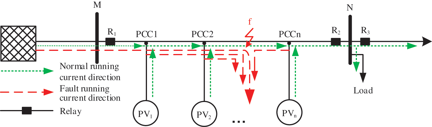
Figure 7: Fault current characteristic of distribution network with PVs

For a given distribution network model with PVs, the location of PVs, the topology of the network, and the system parameters are known. As illustrated in Fig. 7, the protection device is installed at the beginning of the line, and the values of voltage UM and current IM that pass through the protection device can be measured in real time. The voltage drop between the protection device and the first PV connection point PCC1 can be calculated with the measured voltage and current according to Kirchhoff’s voltage law and the connection point voltage of the first PV can be calculated accordingly. Since the LVRT controlling method is known, the output characteristic of the PV can be deduced with the PV connection point voltage.

The magnitude of the injected current at different PV connection points can thus be calculated based on the LVRT capacity. The calculation of the injected current at the PV connection point is shown in Fig. 8.

Figure 8: Virtual measurement current calculation process

The fault current I˙2 equals the superposition of the output current of the PV I˙PV and the measured current I˙M. If more than one PV is connected, the connection point voltages and feeding currents of all PVs PV1, PV2, …, and PVn can be deduced one by one with topology and voltage drops along the transmission line. This process is illustrated in Eq. (5).

{U˙pccn=U˙pccn−1−(∑j=1n−1I˙PVi+I˙M)Zn−1I˙PVn=f(U˙pccn)(5)

The current at the end of the line calculated via this process is called virtual measurement current.

3.2 Virtual Measurement Current under Normal Operation and External Faults

During normal operation, the circuit of the distribution network with PVs is shown in Fig. 9.

Figure 9: Equivalent circuit diagram under normal operating conditions

In normal operation, Kirchhoff’s current law is satisfied when the current on both sides of the protection zone and the output currents of PVs are considered. The downstream virtual measurement current ik is defined as the sum of the measured current im at the beginning of the line and the output current iPVi(i=1,2,⋯,n) of all PVs within the protection zone, as shown in Eq. (6). Therefore, virtual measurement current ik and measured current in are almost the same since the Kirchhoff’s current law must keep. When the load state is ignored, the relationship between the actual measured differential current at the end of the line and the compensation current satisfies Eq. (7).

ik=im+iPV1+iPV2⋯+iPVn(6)

in−ik≈0(7)

When an external fault occurs beyond the protection zone, the equivalent circuit diagram is shown in Fig. 10.

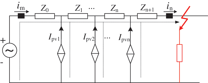
Figure 10: External fault equivalent circuit diagram

The currents at both protection zone boundaries and the output current of the PVs also satisfy Kirchhoff’s current law, as shown in Eq. (8).

im+iPV1+iPV2⋯+iPVn=in(8)

3.3 Virtual Measurement Current under Internal Faults

Fig. 11 shows the equivalent circuit diagram of a transmission line when a fault occurs between PVx−1 and PVx. For internal faults, the measured current in of the protection device N is mainly the current fed into the fault point by the downstream PVs, as shown in Eq. (9). The fault current component provided by the system is much larger than that provided by PVs. However, due to the uncertainty of PVs and the unmeasured current of the fault point, the relationship between the currents on both sides of the protection zone does not satisfy the Kirchhoff current law. At this time, the correlation between the virtual measured current and the current at the end of the line is relatively low, and Eq. (7) is not satisfied.

iPVx+iPVx+1⋯+iPVn=−in(9)

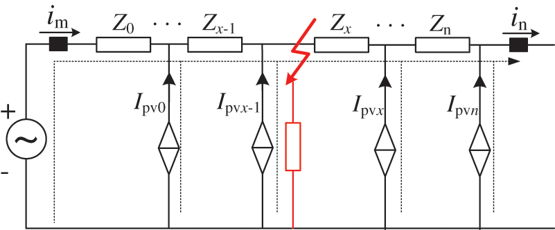
Figure 11: Internal fault equivalent circuit diagram

4  Distribution Line Longitudinal Protection Method Based on Virtual Measurement Current Restraint

4.1 Edit Distance Algorithm

This article proposes an improved edit distance on a real sequence (EDR) algorithm to quantitatively compare the similarity between two waveforms [20–22].

The editing distance refers to the minimum number of editing operations required to convert one to the other between two strings. For two tracks tr1 and tr2 with given lengths of m and n, respectively, the matching threshold of the minimum distance is ε. The EDR distance between two tracks is defined to be the minimum number of operations that are required to insert, delete, or replace tr1 to transform it into tr2. Its operation steps are as follows.

Firstly, an edit distance matrix D of size (m+1)×(n+1) for tr1 and tr2 is established, and the element d(i,j) in matrix D is defined. Then, to facilitate the subsequent calculation of different matrix values, the edit distance matrix is initialized. The first row and column of matrix D represent the editing distance between an empty string and a non-empty string, that is the length of the empty string. Finally, the sequence is subjected to three operations, namely insert, delete, and replace operations, to complete the conversion from tr1 to tr2. The explanations of these three kinds of operations are as follows:

(1) Insertion: Insert the jth character of tr2 after the (i-1)th character of tr1, that is, add 1 on the basis of d(i−1,j). At this time, the value of d(i,j) is d(i−1,j)+1.

(2) Deletion: Delete the ith character of tr1, that is, add 1 on the basis of d(i,j−1). At this time, the value of d(i,j) is d(i,j−1)+1.

(3) Replacement: Replace the ith character of tr1 with the jth character of tr2, that is, add 1 on the basis of d(i,j−1), and at this time, the value of d(i,j) is d(i−1,j−1)+1. Note that, if the difference between the two elements tr1i and tr2j is less than the threshold ϵ, the two elements are considered similar, and no operation is performed.

Therefore, the expression for the edit distance can be obtained as shown in Eq. (10).

dEDR(i,j)={ max(i,j)min{ dEDR(i−1,j)+1dEDR(i,j−1)+1dEDR(i−1,j−1)+Δdmin(i,j)=0min(i,j)≠0(10)

Among them, the expression of penalty coefficient Δd is given by Eq. (11).

Δd={ 01d(tr1i,tr2j)≤εd(tr1i,tr2j)>ε(11)

where, d(tr1i,tr2j) is the difference between the ith value in the track tr1 and the jth value in the track tr2, and ε is the set threshold.

Then, the similarity of the two groups of sequences can be calculated as Eq. (12).

Dedt=1−dEDR(m,n)max(LA,LB)(12)

If the EDR algorithm threshold is set as 0.05, m = n = 10. The two sequences tr1 and tr2 are set as examples for calculation, and the corresponding sequence timing diagram is shown in Fig. 12.

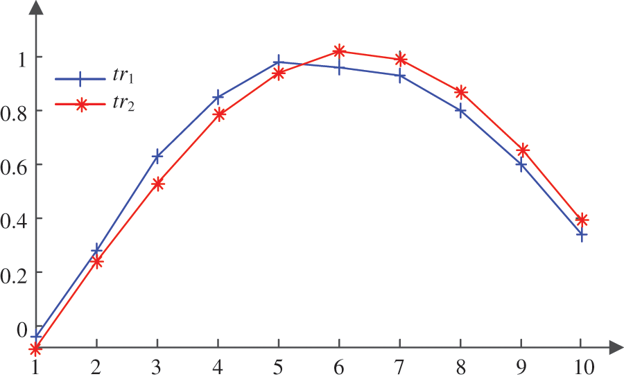
Figure 12: Sequence diagram of two data sequences

According to the calculation method of the improved editing distance, 1 is added to the editing distance value when its value is larger than the threshold. The smallest value between the two paths is taken, and the specific path matrix, as shown in Fig. 13, is drawn.

Figure 13: Path matrix

The similarity can be calculated as Dedt=1−6÷10=40%. According to the definition of EDR, it can be found a smaller edit distance value suggests a higher waveform similarity.

4.2 Protection Method and Setting

The edit distance is used to judge the similarity of two current waveforms, and the edit distance similarity value between the virtual measurement current and the current at the load end of the protection line is used to construct the protection criterion, as shown in Eq. (13).

{Dedt>DsetExternal faultDedt<DsetInternal fault(13)

Here, Dedt is the edit distance similarity between the virtual measurement current and the fault current at the load end of the protection. Dset is the setting value of editing distance similarity. Such setting value should be small enough to avoid the maximum unbalanced current of external faults. Its value is determined by dividing the lowest similarity of maximum unbalance current with the reliable coefficient which is usually between 1.05 and 1.1.

4.3 Protection Method Process

In this paper, a differential protection method based on virtual measurement current is proposed. The protection process is shown in Fig. 14. Both the voltage and current of the source side and only the current of the load side are collected and used for the proposed protection algorithm. The current waveform of the load side can be deduced from the voltage and current collected at the source side. The time window of the collected data is 0.04 s. The proposed protection method includes the following steps:

Figure 14: Protection method flow chart

(1) Protection start-up criteria

Since the real-time calculation of the virtual measurement current involves a large computation, voltage fluctuation is used to start the protection criterion. The protection is activated when the voltage satisfies the equation ΔU>Uop_set.

(2) Calculation of virtual measurement current

After the protection is activated, the voltages and currents at both sides of the protection zone are collected for a certain time, and the real-time power output of PVs in the protection zone is calculated to obtain the virtual measurement current ik.

(3) Calculation of edit distance

The edit distance between the virtual measurement current and the load-side current is calculated as shown in Eq. (12), and the protection is judged according to the criteria in Eq. (13). When the similarity between the two edit distances is greater than the threshold Dset, it is determined to be an external fault. Otherwise, it is determined to be an internal fault.

5  Simulation Results and Analysis

The IEEE 33-node model is built on the simulation platform of PSCAD as shown in Fig. 15. The PV source has a rated capacity of 2 MVA. The protection zone is between node 26 and node 30. Node 26 is denoted as the source end (M end) and node 30 is denoted as the load end (N end), and PV1 is connected to node 29 and PV2 is connected to node 32. Internal fault f1, external downstream fault f2, and external upstream fault f3 are set to verify the effectiveness of the proposed protection method. The sampling frequency is set as 2 kHz. The simulations show the maximum unbalanced current similarity of external faults ranges from 0.85 to 1. To ensure the reliable operation of protections, a reliable coefficient of 1.05 is used to set the threshold of Dset, that is Dset=0.85/1.05=0.8.

Figure 15: Topology of the simulated IEEE-33 node system

5.1 Case Study

When the fault occurs at the f2 location, the actual fault currents measured at M and N are shown in Fig. 16a. Due to the feeding current of PV, there is a certain difference between the fault currents measured at both ends of the protection zone, which results in low similarity of two current waveforms. The virtual and actual currents at node 31 are obtained as shown in Fig. 16b after compensation. It is clear that the compensation is effective when an external fault occurs.

Figure 16: Currents of both ends of the protection zone. (a) Current waveform of external fault before compensation, (b) Current waveform of external fault after compensation

When an internal fault f1 occurs, the measured current at both ends of the protection zone is shown in Fig. 17a. The compensated current waveform and the actual measured current waveform at the load side are shown in Fig. 17b. It can be seen that for an internal fault, there is a significant difference between the actual currents from both sides, which results in a low similarity between the virtual compensation current and the current at the load side. The internal fault changes the equivalent fault circuit, and only the currents from both ends cannot fulfill Kirchhoff’s current law. The unbalanced current of the PV enhances the difference between the virtual compensation current and the actual measured current at the load side, which validates the effectiveness of the proposed protection method.

Figure 17: Currents of both ends of the protection zone. (a) Current waveform of internal fault before compensation, (b) Current waveform of internal fault after compensation

The operation time of the virtual current calculation algorithm is 0.1395 s. The protection exit time is the sum of the collection time and the operation time. As the collection time is the length of the data window, 0.04 s, the total protection time is 0.1795 s.

5.2 Effect of Resistance

Practically, the fault resistance will be different for different faults. Fig. 18 shows the simulation waveforms of actual currents at the load side and compensated currents when external faults with different resistances are considered.

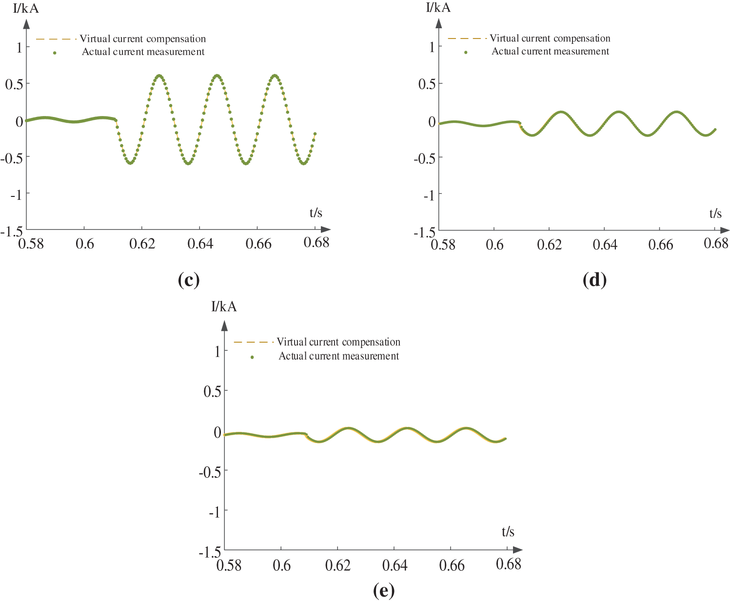
Figure 18: Influence of different transition resistors on compensation current of external fault, (a) Rf = 2 Ω, (b) Rf = 5 Ω, (c) Rf = 10 Ω, (d) Rf = 30 Ω, (e) Rf = 50 Ω

Similarly, the simulation waveforms of actual currents at the load side and compensated currents when internal faults with different resistances are considered are shown in Fig. 19.

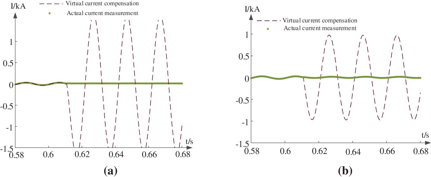
Figure 19: Influence of different resistors on compensation current of internal faults, (a) Rf = 2 Ω, (b) Rf = 5 Ω, (c) Rf = 10 Ω, (d) Rf = 30 Ω, (e) Rf = 50 Ω

The resistors from 1 to 50 Ω are set respectively at fault locations f1, f2, and f3, and the protection results are shown in Fig. 20.

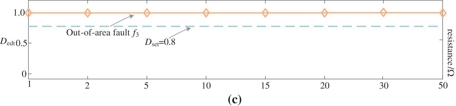
Figure 20: Waveform similarity values of faults at different locations and resistances, (a) fault occurs at f1, (b) fault occurs at f2, (c) fault occurs at f3

The results show that the performance of the proposed protection method is immune to the effect of resistance even when the resistance reaches 50 Ω. The fault characteristics are obvious when the transition resistance is below 10 ohms. When the transition resistance becomes higher, the voltage drop will be smaller and the effect of PV will decrease. The performance of the proposed protection method will be better.

5.3 Effect of Noise

Noise interference is commonly found during sampling. The increase in threshold can improve the denoising capability of the edit distance similarity comparison method. The difference between the points in the sequence is compared with the threshold ϵ. Based on the comparison result, it is determined whether the edit distance should be increased by 0 or 1. With the influence of noise interference and outliers, if the matrix element d(xi,yj) is greater than the threshold, the edit distance value will increase.

If the threshold is too large, the calculated edit distance value will become larger and will cause high waveform similarity when there is an internal fault. The protection does not operate. On the other hand, if the threshold is too small, the waveform similarity between compensated waveforms of external faults will also decrease. The protection method might malfunction.

As most background noises are Gaussian noises, the wavelet threshold de-noising method is widely used due to its easy implementation and preservation of the original signal characteristics [18,19]. In this paper, Gaussian white noise is added to the signal according to different signal-to-noise ratios (SNRs), which can be calculated as shown in Eq. (14).

SNR=10log10⁡PsignalPnoise=10log10⁡∑x2∑n2(14)

where, x is the raw signal data, n is the noise data.

In this paper, wavelet transform is used to process the noisy waveform. The de-noising diagram is shown in Fig. 21. When wavelet threshold de-noising is used, it is necessary to select a suitable wavelet basis function and decomposition level and perform wavelet decomposition on the noisy signal to obtain the wavelet coefficients. Then, the high-frequency coefficients of the wavelet decomposition are quantized by threshold. Finally, the de-noising signal is obtained by wavelet reconstruction. Therefore, the threshold is set to be ε = 0.01 concerning the practical 10 kV distribution network current level.

Figure 21: Schematic diagram of wavelet threshold noise reduction

The selection of a wavelet base is also discussed in this paper. Daubechies wavelets and symmetric wavelets are sensitive to irregular signals such as sudden faults, and have tight support and orthogonal characteristics. They are suitable for processing faulted sinusoidal waves with noise. Different wavelets are tested with simulated signals and the results are listed in Table 1. The same fault signal is added with Gaussian white noises with an SNR of 20 dB. The de-noising performance is evaluated by root mean squared error (RMSE) between the denoised signal and the original one. As illustrated in Table 1, the “db4” wavelet has better performance and is thus selected.

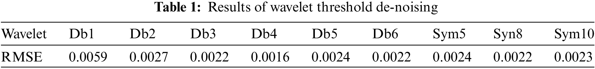
The denoising performance of the “db4” wavelet is illustrated in Fig. 22. Here, 20 dB noise is added. It can be seen from the figure that the noise component is significantly reduced. The use of db4 wavelet threshold de-noising can effectively eliminate the influence of noise on the original waveform.

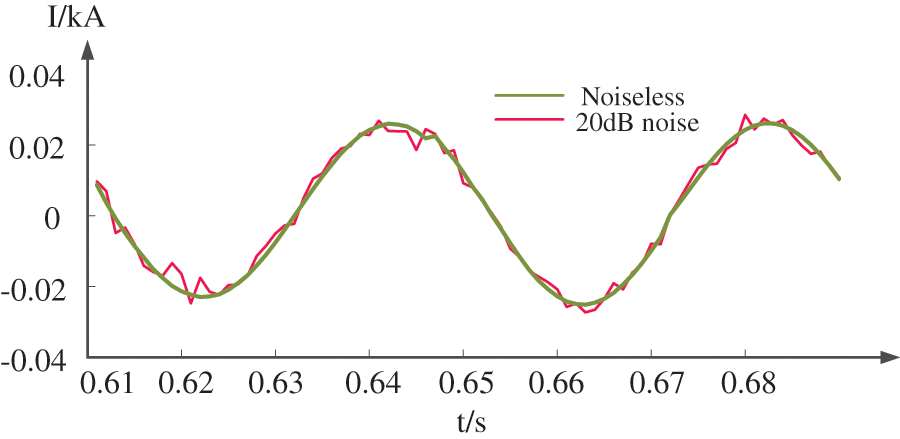
Figure 22: Line Noise Effects

When the collected current data contains noise, it will affect similarity discrimination. Therefore, wavelet de-noising is used to eliminate high-frequency noise in the sampling process. Noises from 20 to 40 dB are added at the fault locations f1, f2, and f3. The corresponding protection results are shown in Fig. 23.

Figure 23: Waveform similarity value of different position faults and different noise interference, (a) fault occurs at f1, (b) fault occurs at f2, (c) fault occurs at f3

From Fig. 23, it can be seen that for different types of internal faults, the similarity calculated by the proposed protection method is lower than the threshold under noise interference from 20 to 40 dB, and it is determined to be an internal fault. For different types of external faults, the similarity between the compensated virtual currents and the actual currents can still be higher than the threshold, and they can be determined to be external faults. Therefore, the proposed protection method can tolerate a certain level of noise interference.

5.4 Effect of Time Error

Time error is commonly found when data collections from both ends are not synchronized. To deal with this kind of problem, the waveforms from the source end and compensated waveforms from the load ends are processed. The lagging part of the lagging waveform is cut and moved to the head of the lagging waveform. The editing distance of the processed waveforms is calculated and compared. The specific process is shown in Fig. 24.

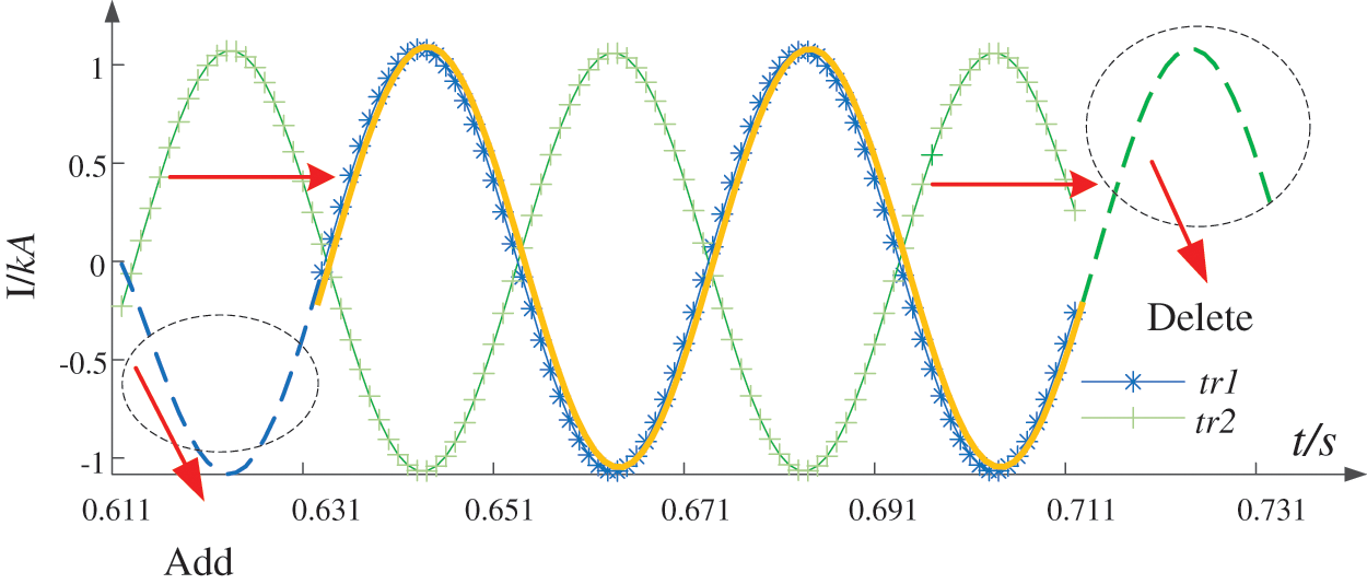
Figure 24: Processing of lagging waveform with time errors

Firstly, the add operation is performed on the sequence tr1, and tr1 is aligned with the starting point of tr2. Secondly, the translation operation is performed on the tr2 curve to translate the number of steps added by tr1 and delete the redundant sequence. Finally, the similarity is calculated by comparing the preprocessed parts. The alignment of the preprocessed waveform data is shown in Fig. 25.

Figure 25: Time synchronization of waveform data after preprocessing

The algorithm proposed in this paper calculates the similarity by comparing the edit distance of two waveforms. When the data are not synchronized due to the communication delay, the two waveforms will not match and the similarity will reduce. For internal faults, unsynchronized data has little effect on the protection, while for external faults, it may cause malfunction of protection. To verify the impact of unsynchronized data during external faults, Fig. 26 shows the protection actions from 1% to 20% of unsynchronized data when faults occur at locations f1, f2, and f3.

Figure 26: Waveform similarity values of faults at different locations and different unsynchronized ratios, (a) fault occurs at f1, (b) fault occurs at f2, (c) fault occurs at f3

From Fig. 26, it can be seen that when the unsynchronized data ratio reaches 20%, the similarity calculated for internal faults is always lower than the threshold, and the protection will operate. For external faults, the similarity between virtual current and actual current can still be higher than the threshold, and it is determined to be an external fault and the protection does not trip. Therefore, this protection method can tolerate the impact of time errors.

6  Comparisons

The traditional differential protection method uses the current difference between the two ends of the protected line as the operating value. When PV is connected to distribution networks in the form of a T connection, traditional differential protection cannot work effectively. When faults occur in the protection zone, the current difference between the two ends increases due to the PV feeding current. But when an external fault occurs, the current difference between the two ends of the line is the PV feeding current which is usually larger than the protection threshold. This will cause malfunction of traditional differential protection. The proposed protection method based on virtual measurement current compensates the load side current by calculating the output current of T-connected PVs in real-time, which not only eliminates the unbalanced current at both ends when the fault occurs outside the protection zone but also improves the braking effect of the protection when the fault occurs inside the protection zone. Fig. 27 shows the results of traditional differential protection and proposed protection with different PV interconnection capacities and different resistances.

Figure 27: Action results of traditional differential protection and proposed protection. (a) Different PV access capacities. (b) Different resistances

As illustrated in Fig. 27a, for external faults, when the PV capacity increases, the PV feeding current increases to the maximum unbalance current of the line, and the protection will misoperation. As shown in Fig. 27b, the proposed protection method can correctly calculate the PV feeding current and make compensation when the PV capacity gradually increases. The similarity of current waveforms at both ends is above the similarity threshold, and the protection is still reliable and does not operate. When internal faults with higher resistances, the fault current is the fault current provided by PV. For the traditional differential protection, the current difference is small, and the protection cannot operate. The protection method proposed not only compensates for the PV effect, but also enhances the difference of the current at both ends, and its similarity can still be less than the threshold value, so the protection acts correctly. In summary, the proposed protection method can correctly operate with large amounts of PVs, but the traditional differential protection cannot operate correctly when external faults and high-resistance internal faults occur.

The proposed protection method has many advantages, such as high reliability and strong tolerance to transition resistance. The editing distance algorithm eliminates the effect of time error and has advantages in low protection cost.

7  Conclusion

In this paper, a distribution line longitudinal protection method is proposed to deal with the problems of large-scale PV interconnections. Virtual current compensation is used to illuminate the effect of PVs during faults. After compensation, the currents from both ends of the protected zone can be used directly for differential protection and the effect of PVs can be restrained. An editing distance algorithm is proposed to compare the virtual measured current with the actual measured current and achieve reliable differential protection.

This method has high sensitivity and is robust to the presence of noise and time errors. By using the wavelet de-noising method, it can tolerate Gaussian noise up to 20 dB, and by utilizing the improved edit distance for data deletion operations, it can tolerate data delay errors up to 20%. The proposed method is not affected by resistance and fault type. Compared with the existing two-terminal or multi-terminal differential protections, this method needs to install a current transformer and voltage transformer at the source end and only a current transformer at the load end, which is easy to implement in practical scenarios. Compared with the three-section current protection which is commonly used in distribution networks, the proposed method can operate reliably and quickly. Therefore, the proposed method has a high potential to be used in distribution networks with large-scale interconnections of PVs and is possible to improve the protection performance.

Acknowledgement: This work was supported by the Anhui Power Grid Co., Ltd. and Professor Guomin Luo’s group of the School of Electrical Engineering of Beijing Jiaotong University.

Funding Statement: This work was funded by State Grid Anhui Electric Power Co., Ltd. Science and Technology Project (52120021N00L), and the National Key Research and Development Program of China (2022YFB2400015).

Author Contributions: The authors confirm contribution to the paper as follows: study conception and design: Wei Wang, Yang Yu, Simin Luo and Wenlin Liu; data collection: Wei Tang and Yuanbo Ye; analysis and interpretation of results: Wei Wang, Simin Luo and Wenlin Liu; draft manuscript preparation: Yang Yu and Simin Luo. All authors reviewed the results and approved the final version of the manuscript.

Availability of Data and Materials: Data supporting this study are included within the article.

Conflicts of Interest: The authors declare that they have no conflicts of interest to report regarding the present study.

References

1. Tan, X. D., Liu, J., Xu, Z. C., Yao, L., Ji, G. Q. et al. (2021). Power supply and demand balance during the 14th five-year plan period under the goal of carbon emission peak and carbon neutrality. Electric Power, 54(5), 1–6. [Google Scholar]

2. Kim, G. C., Ibraheem, W. E., Ghani, M. R. A. (2014). Impact of photovoltaic (PV) systems on distribution networks. International Review on Modelling and Simulations, 7(2), 298–310. [Google Scholar]

3. Emmanuel, M., Rayudu, R. (2017). The impact of single-phase grid-connected distributed photovoltaic systems on the distribution network using P-Q and P-V models. International Journal of Electrical Power & Energy Systems, 91, 20–33. [Google Scholar]

4. Soroudi, A. (2012). Possibilistic-scenario model for DG impact assessment on distribution networks in an uncertain environment. IEEE Transactions on Power Systems, 27(3), 1283–1293. [Google Scholar]

5. Song, Y., Hill, D. J., Liu, T. (2019). Impact of DG connection topology on the stability of inverter-based microgrids. IEEE Transactions on Power Systems, 34(5), 3970–3972. [Google Scholar]

6. Vovos, P. N., Kiprakis, A. E., Wallace, A. R., Harrison, G. P. (2007). Centralized and distributed voltage control: Impact on distributed generation penetration. IEEE Transactions on Power Systems, 22, 476–483. [Google Scholar]

7. Hamed, H., Seyed, M. M., Hossein, A., H, H. (2016). Sensitivity analysis of smart grids reliability due to indirect cyber-power interdependencies under various DG technologies, DG penetrations, and operation times. Energy Conversion and Management, 108, 377–391. [Google Scholar]

8. Lin, X. N., Ma, X., Wang, Z. X., Sui, Q., Li, Z. T. et al. (2021). A novel current amplitude differential protection for active distribution network considering the source-effect of IM-type unmeasurable load branches. International Journal of Electrical Power & Energy Systems, 129(2), 106780. [Google Scholar]

9. Gao, H., Li, J., Xu, B. (2016). Principle and implementation of current differential protection in distribution networks with high penetration of DGs. IEEE Transactions on Power Delivery, 32(1), 565–574. [Google Scholar]

10. Xu, Y. J., Jin, N. Z., Ye, Z. F., Zhu, M., Zhang, Z. C. (2014). Research and application of EPON based clock synchronization protocol in the multi-terminal differential protection of distribution line. Power System Protection and Control, 42(6), 39. [Google Scholar]

11. Lei, J. Y., Li, Z. Y., Lu, Z. H., Xin, H. H., Yang, H. (2011). Review on the research of distributed generation technology and its impacts on electric power systems. Southern Power System Technology, 5(4), 46–50. [Google Scholar]

12. Han, B., Li, H., Wang, G., Zeng, D., Liang, Y. (2017). A virtual multi-terminal current differential protection scheme for distribution networks with inverter-interfaced distributed generators. IEEE Transactions on Smart Grid, 9(5), 5418–5431. [Google Scholar]

13. Zhang, X. A., Tan, Q., Liu, X., Zhou, S. Q., Feng, W. M. (2013). Research on the distribution networks centralized differential protection method based on generalized nodes. Power System Protection and Control, 41(11), 111–116. [Google Scholar]

14. Chisava, O., Ramos, G., Celeita, D. (2022). Time-domain sensitive differential protection approach for high impedance faults (HIF). Industry Applications Society, 28, 1–6. [Google Scholar]

15. Miao, X. R., Zhao, D., Lin, B. Q., Jiang, H., Cheng, J. (2023). A differential protection scheme based on improved DTW algorithm for distribution networks with highly-penetrated distributed generation. IEEE Access, 11, 40399–40411. [Google Scholar]

16. Zhou, C. H., Zou, G. B., Zang, L. D., Du, X. G. (2022). Current differential protection for active distribution networks based on improved fault data self-synchronization method. IEEE Transactions on Smart Grid, 13(1), 166–178. [Google Scholar]

17. Zhou, C. H., Zou, G. B., Du, X. G., Zang, L. D. (2022). Adaptive current differential protection for active distribution network considering time synchronization error. IEEE Transactions on Power Systems, 140, 108085. [Google Scholar]

18. Chen, G. B., Liu, Y. Q., Yang, Y. F. (2020). Impedance differential protection for active distribution network. IEEE Transactions on Power Delivery, 35(1), 25–36. [Google Scholar]

19. Yuan, T., Gao, H. L., Peng, F., Li, L., Zhang, Y. C. et al. (2023). Adaptive Quasi-power differential protection scheme for active distribution networks. IEEE Transactions on Smart Grid, 14, 1. [Google Scholar]

20. Tong, X. Y., Quan, W. J., Li, Z., Xi, J. Y., Dong, X. X. (2023). Backup protection scheme for flexible DC transmission line by traveling wave waveform similarity based on improved editing distance. Power System Technology, 47(1), 294–303. [Google Scholar]

21. Luo, H. Z., Liu, S. J., Gan, Y. J., Li, N., Jiang, H. M. (2023). An OTDR signal denoising algorithm based on CEEMDAN-improved wavelet threshold. Journal of Optoelectronics Laser, 33(3), 241–247. [Google Scholar]

22. Wu, Y. L., Xing, H. Y., Li, J., Zhang, Y. C., Duan, R. J. (2022). Wavelet denoising algorithm with improved threshold function. Journal of Electronic Measurement and Instrument, 36(4), 9–16. [Google Scholar]