GNN Representation Learning and Multi-Objective Variable Neighborhood Search Algorithm for Wind Farm Layout Optimization

Nomenclature

1  Introduction

Wind energy has become one of the fastest-growing and most popular renewable sources in the last few decades. With the depletion of oil resources and the degradation of the environment, wind power has been rapidly developed everywhere and the application of wind energy is increasing in power systems. As a result, different studies have been devoted to this field. Wind farm layout optimization is an important part of wind power development, which is directly related to the economic benefit, environmental impact, and social benefit of wind farms. Therefore, developing a scientific and reasonable wind farm layout is of great importance.

In recent years, wind farm layout optimization has been the focus of research in various countries for the increasing capacity of wind farms. There are several ways to operate wind turbines, among which grid-connected operation is the most economical and effective way to use wind energy on a large scale. In this way, wind turbines are connected to the grid and transmit electricity there, decreasing the capital expenses for equipment and generation [1]. However, power quality at the point of common coupling (PCC) will be affected to some extent by the wind turbine generator (WTG) in grid-connected operation, mostly due to voltage fluctuation and flicker induced by output power variation [2]. Therefore, it is becoming increasingly crucial to research the voltage flicker and power quality caused by grid-connected wind turbines at PCC to ensure the power quality of the system. It can be seen that many technical issues related to wind farms need to be solved. For example, from an economic point of view, the route length of a wind farm needs to be short to reduce construction costs. From the perspective of power quality, the flicker value at the point of common coupling (PCC) needs to be low to improve the quality of wind energy.

Some of the current state-of-the-art methods are used to construct wind farm layout schemes, but they still have some limitations in terms of algorithm performance, and the expressive capability and search performance of the model can be further improved.

Considering the limitations we mentioned before, a multi-objective optimization framework with GNN representation learning and Variable Neighborhood Search (VNS) algorithm is proposed as the best scheme for wind farm layout optimization with economic and power quality objectives. GNN representation learning is used to preprocess data, which can improve expressive capability, while the multi-objective VNS algorithm can help improve search efficiency and accuracy in multi-objective problems. The main contributions include three aspects:

(1) The layout optimization problem of wind farms is defined, and several optimization objectives are proposed to convert it into a multi-objective optimization problem in mathematics.

(2) In order to improve the efficiency and accuracy of the algorithm, GNN representation learning is introduced to preprocess graph data, so that the initial node set of the VNS algorithm can be constructed.

(3) A multi-objective variable neighborhood search algorithm is proposed by combining a multi-objective optimization algorithm with VNS, which helps to improve the expressive capability and search performance in multi-objective optimization problems.

The rest of the paper is organized as follows: Section 2 provides related works. The definition of the wind farm layout optimization problem is explained in Section 3. Section 4 proposes an efficient method with GNN representation learning and a multi-objective variable neighborhood search algorithm. Case studies and their simulation results are given in Section 5. Section 6 presents conclusions.

2  Related Works

In recent years, wind farm layout optimization has been the focus of research in various countries due to the increasing capacity of wind farms. There have been many studies on the layout optimization of wind farms. In 2018, Sorkhabi et al. [3] combined multi-objective continuous variable genetic algorithms (NSGA-II) with novel constraint processing methods, using a combination of penalty functions and constraint programming to balance local and global exploration and solve optimization problems. In 2019, Ju et al. [4] proposed a support vector regression-guided genetic algorithm to solve the wind warm layout optimization problem, which has been validated under different settings of wind distribution and wind farms with unusable cells. Yang et al. [5] developed a wind farm layout optimization method based on simulated annealing, and the performance of the algorithm was evaluated by comparing it to those of previous studies under three wind scenarios. In 2020, Reddy et al. [6] proposed a new framework for wind farm layout optimization with the goal of maximum annual energy production. In 2021, Moreno et al. [7] used a multi-objective lightning search (MOLS) algorithm and compared it with multiple multi-target algorithms to demonstrate the efficient performance of the multi-target lightning search algorithm in wind farm layout optimization. Verma et al. [8] used the improved multi-objective genetic algorithm (MOGA) to successfully reduce the loss of the power distribution process in the wind farm and improve the performance of the wind farm. Dhoot et al. [9] presented a novel method with probabilistic inference to quickly generate approximate optimal layouts for maximum energy production. In 2022, Cazzaro et al. [10] developed a variable neighborhood search method for the layout planning of large-scale offshore wind farms, considering in addition the minimum distance constraint and foundation costs. More recently, Rizk-Allah et al. [11] proposed a novel algorithm based on the hybridization of equilibrium optimizer (EO) and pattern search (PS) techniques and implemented it to deal with wind farm layout optimization using different wind speed scenarios.

3  Definition of Wind Farm Layout Optimization Problem

3.1 Model of Wind Farm Output

The wind speed probability distribution can help describe the wind energy resources of a wind farm, and the output power can then be calculated. In this paper, we adopt the wind speed and wind direction model of conditional dependence, where conditional dependence refers to the dependence relationship between wind speed and wind direction in a single wind farm. The wind speed is simulated by the two-parameter Weibull model [8–10], and the probability density function is shown as follows [11]:

f(v)=kc(vc)k−1exp⁡(−(vc)k)(1)

where v is the actual wind speed, c and k are the scale and shape parameters of the model, respectively, which c plays the role of enlarging or shrinking the curve and k determines the basic shape of the distribution density curve.

The relationship between active power output of wind turbine and wind speed can be expressed as:

P={00<v<vin or v>voutv−vinvr−vinPrvin≤v<vrPrvr≤v≤vout(2)

where vin,vout is the cut-in and cut-out wind speed, vr is the rated wind speed, and Pr is the rated output of the fan. The process is a monotone nonlinear transformation of the wind speed series. The fan output can be obtained by bringing the wind speed series into the fitting function of the fan output characteristic.

3.2 Model of PCC Flicker Value

Wind power generation will have a negative effect on the quality of the power grid because of the fluctuating nature of wind resources and the ways in which wind turbines operate. The output power will also fluctuate with the switching operation and continuous operation of grid-connected wind turbines, which will further cause voltage fluctuations and flicker [12].

According to the regulations in IEC61400-21, in order to evaluate the voltage fluctuation caused by a single wind turbine [13], the flicker value generated by a single WTG can be calculated as follows:

Plt=c(φ,va)SnSk(3)

where φ is the impedance angle of the equivalent impedance of the power grid at PCC, va is the annual average wind speed at a given hub height, ci(φ,v) is the flicker coefficient of a single WTG at PCC, Sn is the rated capacity of a single wind motor, and Sk is the short-circuit capacity of the wind turbine at PCC.

Due to the different positions of the wind turbines in the wind farm, the wind speed will be variable, so we can use the average method to calculate the flicker value generated by multiple fans connected to the same common connection point as below:

PltΣ=1Sk∑i=1Nw[ci(φ,va)Si]2(4)

where Si is the rated apparent power of a single generator and Nw is the number of WTG connected to PCC.

3.3 Problem Definition of Wind Farm Layout Optimization

The wind farm layout optimization problem refers to the construction of routes for wind farms with operational and other constraints. As explained before, it is hard to obtain a solution through traditional optimization techniques due to their discrete nature and the difficult-to-calculate objective function. This kind of problem has natural interpretations as graphs, so we describe it with a graph as follows.

We consider a route network, denoted by the graph G=(N,A), where N is the set of nodes and A is the set of links representing the routes. We assume that the given route network is undirected. Now the layout optimization problem becomes a multi-constraint problem in graphs. The goal of it is to propose the best network structure to minimize investment and operation costs while satisfying the constraints of system security.

The system will benefit economically from large-scale wind generation, but there will also be many difficulties with the grid’s power quality that cannot be overlooked. The objective function of this paper, which considers power quality indicators, is to minimize the total length of the line and the flicker value at the public access point PCC of the wind farm. The objective function can be described as follows:

{minf1=∑a=1N(∑b=a+1NLa,bna,b)minf2=PltΣ(5)

where f1 is the total length of network lines; f2 is the flicker value at PCC; La,b is the length of a branch between nodes; Na,b is the number of branches between nodes; PΣ is the flicker value at PCC of the wind farm. Our objective is to find a set of routes RS such that objective functions are minimized.

Additionally, the solution must satisfy the real-world constraints. The constraints of wind farm layout optimization mainly include power system flow and route load constraints [14]. To build a chance-constrained model for power grid planning, the principle is to keep the likelihood of the system functioning within the line capacity limits within an acceptable range. The principle is to keep the probability of the system operating within the line capacity constraints within an acceptable range. These specific limitations are as follows.

(1) Power system flow constraint:

{Pl,min≤Pl≤Pl,maxNa<l<Na+NbtlPl,min≤Pl≤tlPl,max1<l<Na(6)

According to Eqs. (2) and (4), the distribution of wind turbine output and required load in the power grid can be determined, then we can obtain the probability distribution of active power system flow on all routes.

In Eq. (6), Na is the number of candidate lines, and the index range of the candidate lines is 1≤l≤Na; Nb is the number of existing branches, and the index range of the existing branches is Na≤l≤Na+Nb; tl indicates whether the line l is under construction, 1 means under construction, 0 means not under construction; Pl,min and Pl,max are correspond to the lower and upper bounds of the branch power.

(2) Route load constraint:

P{Pa,b≤P¯a,b}≥α,ab∈Ol(7)

where P{} is a probability event which means the probability that the line will not pass the load should be greater than a certain probability, a,b refers to all lines between node a and node b, Pa,b is the transmission power between a and b, p¯a,b is the maximum transmission power between a and b, and Ol is the set of branches.

Similarly, by calculating Eqs. (2) and (4) from the wind farm output model and PCC flicker value model, we can determine the probability of line overload according to the maximum allowable transmission power limit.

4  GNN Representation Learning and Multi-Objective Variable Neighborhood Search Algorithm for Wind Farm Layout Optimization

The main problem for the stage of the wind farm layout optimization algorithm is low efficiency and search precision. To solve this problem, we propose a route network design algorithm based on a graph neural network and the VNS algorithm, which effectively improves the accuracy of the algorithm.

As shown in Fig. 1, the model consists of two modules: graph representation learning and the multi-objective VNS algorithm. The details of each block will be described in detail in the following sections. In this paper, graph representation learning can be used to get an effective representation of graph nodes. Then we propose to combine it with the multi-objective optimization algorithm to help us solve the multi-objective layout optimization problem with graph data.

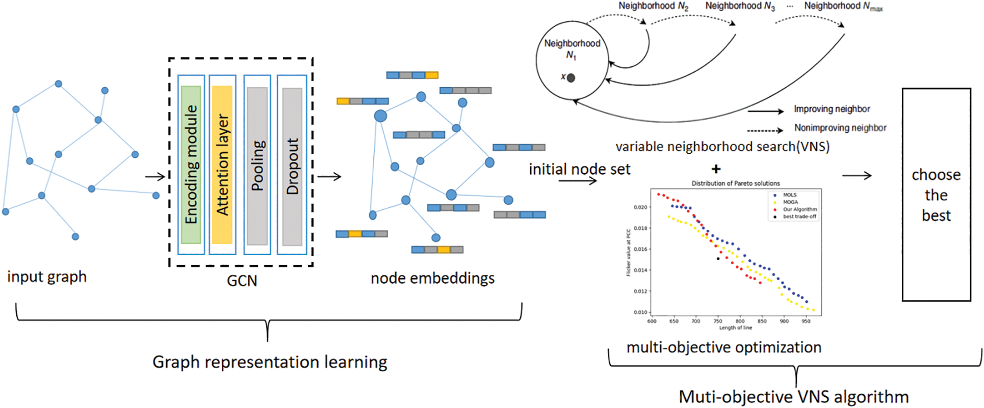
Figure 1: Model structure for wind farm layout optimization problem

4.1 Graph Representation Learning

As many problems have natural interpretations as graphs, one popular approach that has been proposed is to use GNN to solve them. In this paper, we construct and train a graph convolutional neural network to obtain the representation of nodes on wind farm layout optimization problems. For the wind farm route networks, give the following information: (i) Network data (i.e., how the nodes of the network are, the latitude and longitude information of nodes); (ii) The direct link of network nodes; (iii) The electricity demand matrix (i.e., electricity demand between nodes in the networks).

In this paper, we construct a graph neural network that is capable of capturing the representations of nodes and constructing the initial node set (namely INS) among the wind farm roads, and the processing flow is presented in Fig. 2. The structure of the model consists of the following parts.

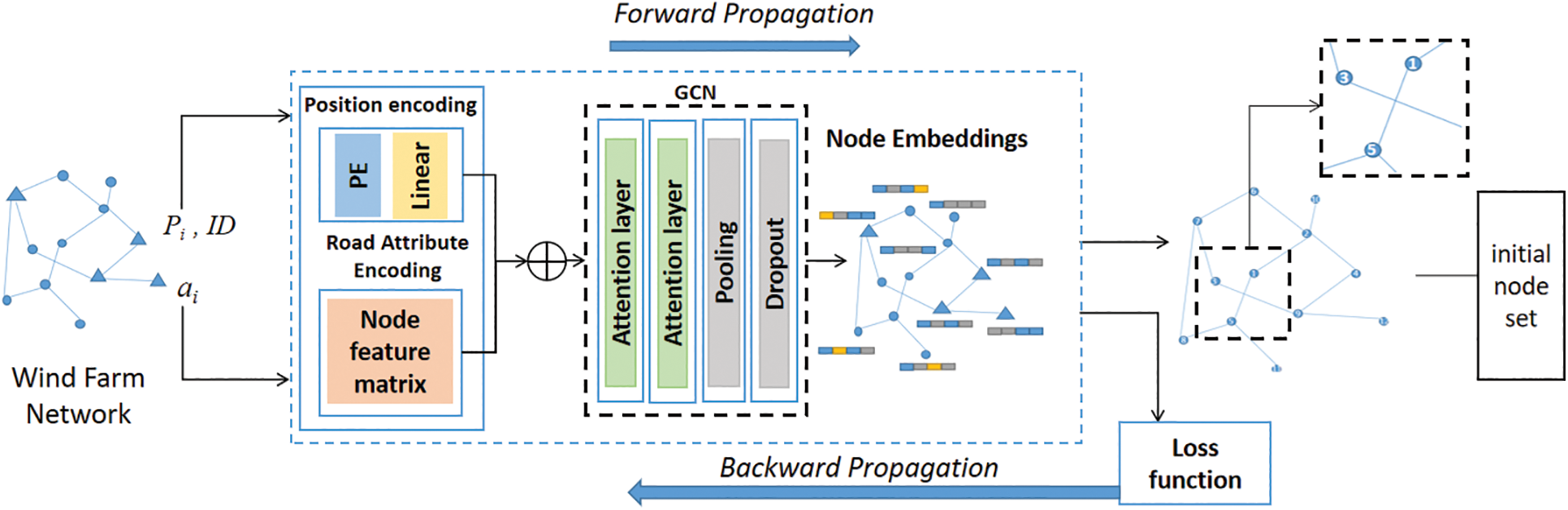
Figure 2: Process of constructing the initial node set with GCN

4.1.1 Encoding

To represent the innate spatial information in wind farm networks, we jointly embed the IDs, positions (including the latitude and longitude information), and attributes of nodes into dense representations as the model inputs. For each road vi, we introduce an embedding layer to encode its ID and position as an embedding vector qi.

Here, an embedding layer corresponds to a Multilayer Perceptron (namely MLP) layer and non-linear function. For node attributes, we clean and normalize the data and combine multiple features into vectors ui for further representation. Finally, for each road, we fuse its positional embedding and attribute embedding into one as follows:

ri=MLP(qi||ui)(8)

where || is the concatenate operation and MLP is a fully connected neural network.

4.1.2 GCN

First, we aggregate the message of each neighbor node huk−1 via the attention mechanism. Then, the message between each target node and its neighbor via a non-linear aggregation function f(v,u) based on the relative position coefficients d(v,u). Finally, the feature output hvk for the target node in the layer can be obtained.

hvk=σ(hvk−1W1(k−1)+∑μ∈N(v)f(μ,v)hμk−1W2(k−1))(9)

where hvk is the representation of node v at the representation of t-th iteration and N(v) is the neighbor set of nodes v. The matrix W1(k−1) and W2(k−1) are trainable weight matrices at the (k–1)-th layer for node v and its neighbors N(v), and the σ means activation function of network. αμ,v means the weight captures via attention mechanism, which can be represented by:

αμ,v=exp⁡(LeakyReLU(aT[Whμ||Whv]))∑k∈Nμexp⁡(LeakyReLU(aT[Whμ||Whk]))(10)

where a(⋅) is a function that calculates the correlation between two nodes, and LeakyReLU means activation function.

4.1.3 Lost Function

Finally, we set the loss function as mean squared error (MSE) function:

MSE(pi,f(Gi;W))=1n∑i=1n[pi−f(Gi;W)]2(11)

where pi represents the power generation of the i-th node, Gi represents the i-th node of the graph G, and W represents the weight matrix to be trained.

4.1.4 INS Construction

To make the proposed algorithm efficient, the initial route sets on which the optimization procedure launches itself must not be arbitrary and be obtained using logical guidelines. Here, each initial route is determined by first selecting the starting node and then selecting all the other nodes sequentially.

The method adopted in this paper is to determine the activity level αi of each node by node degree and select the point with the highest activity level as the initial node. Then, according to the cosine similarity of node i, j obtained by the representation vector in GCN, a probability Pj is assigned to node j, where Pj means the probability of selecting node j on the route until the termination criterion is satisfied. The nodes are sorted from highest to lowest probability and divided into several space intervals, each interval has the same number of nodes. The INS is composed of the nodes, which are randomly selected in the first k intervals.

αi=Degree(i)for i∈G,Pj=hi⋅hj‖hi‖×‖hj‖(12)

where x, y is the representation vector of node i, j, and node i refers to the node before node j.

4.2 Multi-Objective VNS Algorithm

The VNS algorithm is a meta-heuristic algorithm. It explores either at random or systematically a set of neighborhoods to get different local optima [15]. The performance of each of the neighborhoods depends on the initial solution as well as the solution space morphology [10]. The example neighborhood structures for layout in wind farm are as follows (also shown in Fig. 3):

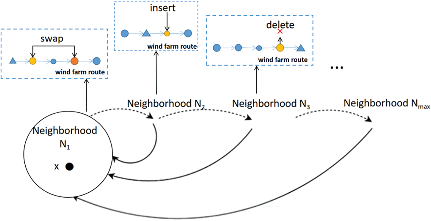
Figure 3: Process of variable neighborhood searching

•   Neighborhood N1: select two random wind power nodes within the wind power network and swap the positions of them on the solution space.

•   Neighborhood N2: insert a node in the solution space subject to the constraints of Eqs. (6) and (7).

•   Neighborhood N3: randomly delete a node from the route in the solution space.

However, this heuristic algorithm tends to fall into local optimality. To prevent this algorithm from stalling, we perform a randomly selected transformation of the optimal solution for ten successive generations. For example, we apply a randomly selected transformation to the current solution for the next three generations. In most cases, alternating between transformational solutions helps prevent stagnation.

Inspired by the combination algorithms such as the multi-objective artificial fish swarm [16,17], we combined the multi-objective optimization algorithm with the above VNS algorithm to judge the quality of the solution with multiple objectives as the objective function to solve the optimization problem. The Tchebycheff approach (Tch) [18,19] is used to determine whether the newly generated solution is reserved. The decomposition-based multi-objective evolutionary algorithm first needs to generate a set of uniformly distributed weight vectors for a weight vector (λ1,…,λm)T, they convert the weight vector as follows:

λ∗=(1λ1∑i=1m,…,1λi∑i=1m1λi)T(13)

As shown in Fig. 4, after this conversion, for the weight vector λ∗, the corresponding solution direction vector along the line of evolution is (λ1,…,λm)T. In addition, a series of wind speeds are generated using the Weibull model, and the output power can be calculated. Each output power corresponds to a scheme to solve the optimal method for reconstructing the route networks.

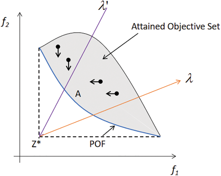
Figure 4: Principle of multi-objective method

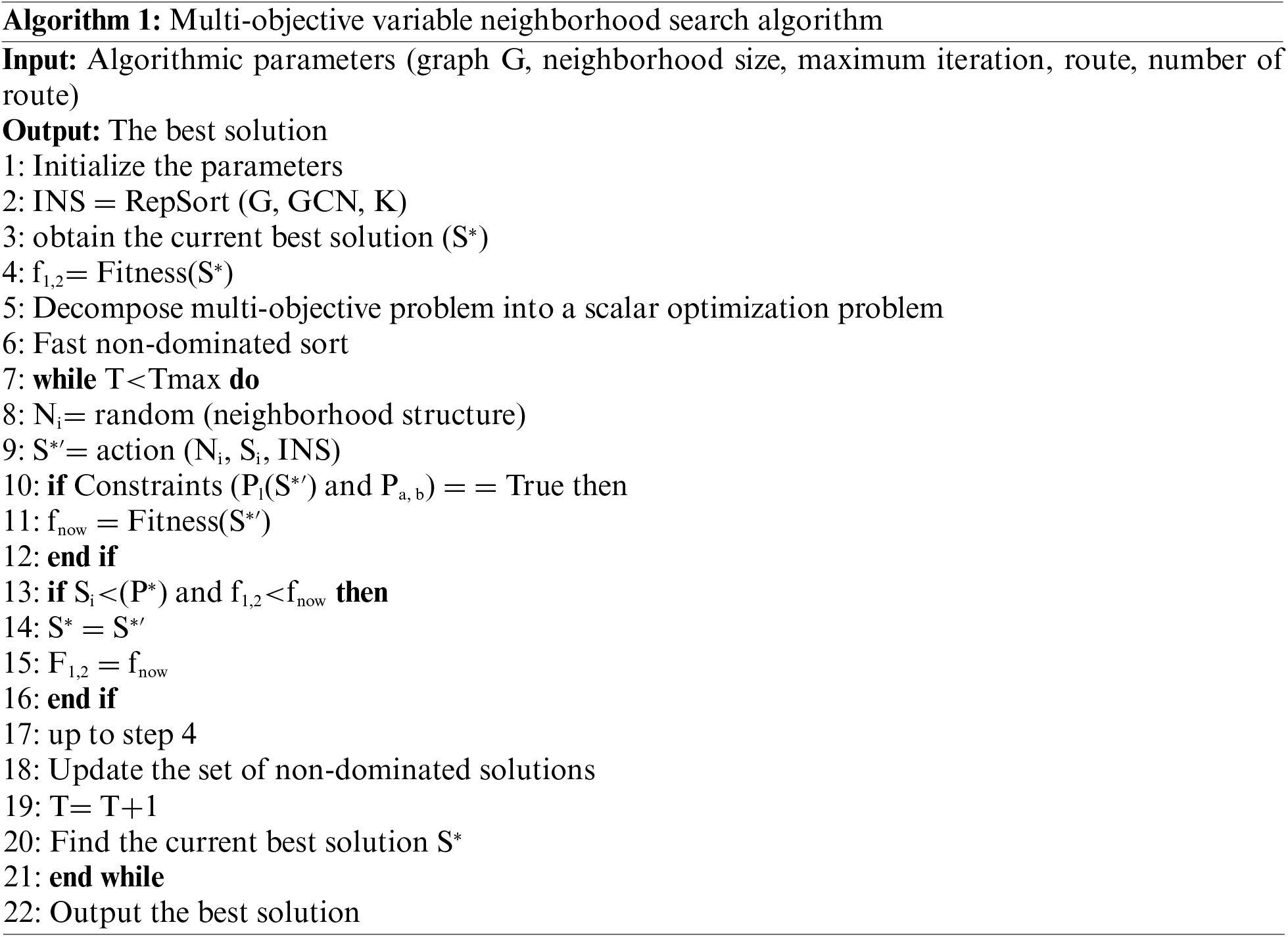
The flow of algorithm 1 is given in the form of pseudo-code. The specific steps are as followsL:

Step 1: Initialize the parameters. Set the number of nodes in the route network as N, the neighborhood structures as N={N1,N2,…,NMAX}, the number of these structures as MAX, the number of routes as R, and establish the maximum number of non-dominated solutions as M.

Step 2: Generate the initial node collection. For the current set of wind farm nodes, the node representation is obtained by training the graph convolutional neural network, and then the initial node set can be generated. The multi-objective function and fitness function of each individual in the initial node set are calculated, and the optimal value is recorded as N.

Step 3: Fast non-dominated sort. Another set K is established, and the non-dominated solution is stored in K by judging the dominance relationship of the solution in set L.

Step 4: Perform behaviors of neighborhood structures. Determine whether the solution is feasible by evaluating Eqs. (6) and (7) of power system flow and route load constraints described in Section 3.3.

Step 5: Determine whether to keep the newly generated solution. Assume that M is the obtained Tch value. After iteration, the Tch value obtained is N. If M>N, it means that the quality of the solution obtained after iteration is better than that before, the corresponding value in the set K will be replaced.

{mingtch(x|λ,z∗)=max1≤i≤m{λi|fi(x)−zi∗|}subject to x∈Ω(14)

where z∗=(z1∗,z2∗,…,zm∗)T is the reference point, For i=1,2,…,m, zi∗=min{fi(x)|x∈Ω}. For a Pareto optimal solution xi∗, there EU must be a weight vector λ that makes xi∗ an optimal solution of the above equation, and every optimal solution corresponds to a Pareto optimal solution of a multi-objective optimization problem. With different weight vectors, we can obtain the corresponding new Pareto optimal solutions.

Step 6: Update the set of non-dominated solutions. According to the numbering order of the nodes, the new solutions are successively updated to perform the non-dominated ranking and update the external set (all Pareto solutions are stored).

Step 7: Update the current best solution. If the fitness value of the solution is better than the current state recorded, the current best state will be updated to the solution state.

Step 8: When the maximum number of iterations is reached, the algorithm ends; Otherwise, go to Step 3.

After the implementation of the algorithm, we can get an optimal wind farm layout scheme. In addition, we can also get the layout under different distances in the iterative process.

5  Experiments

5.1 Dataset

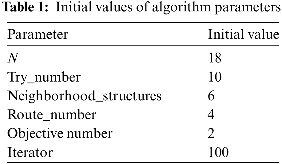
We conducted experiments to evaluate the performance of our improved algorithm in terms of both PCC and operational efficiency. During the experiment, all the details of other parameters are shown in Table 1.

Wind speed as well as angle affect the flicker coefficient of the wind turbine as shown in Table 2. The wind speed in the experiment follows Weibull distribution, and the wind speed at the inlet of the fan is 3 m/s, the rated wind speed is 15 m/s, and the wind speed at the outlet is 25 m/s, regardless of the difference in wind speed distribution of each fan and the correlation between the output wind power and the load power. The wind farm is set up with 18 nodes and 27 pre-selected lines, and the initial roadmap of the 18-node wind power system is shown in Fig. 5. 18-node ensures the credibility and authenticity of the simulation experiment and avoids the inefficiency of the algorithm due to too many nodes.

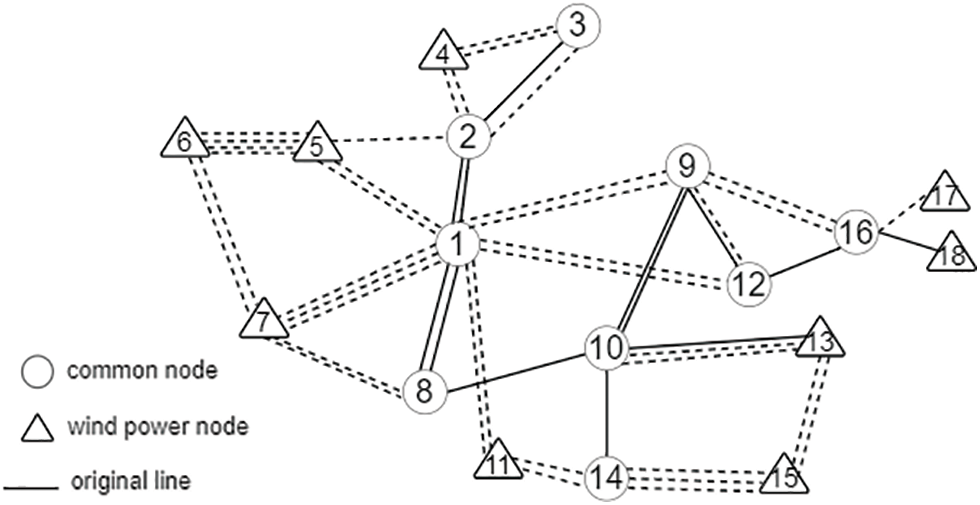
Figure 5: Initial path diagram of 18-node system

The lines in Fig. 5 represent the power transfer requirements between the two wind power nodes in the initial scenario. Assuming that each line makes an equal contribution to the power supply, the optimization process helps us minimize the length of lines and find the best solution that can meet the power demand based on the initial wind farm networks.

The path diagram obtained by using the algorithm is shown in Fig. 6. It can be seen that 21 of the initial 38 optional lines are optimized which can meet the demands of power load, security, and reliability.

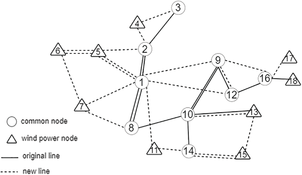
Figure 6: Schematic diagram of optimized path of 18-node system

We selected the MOLS [20] and MOGA [21] algorithms respectively to verify the optimization performance of the algorithms. Table 3 shows the three algorithms with 100 iterations, and Fig. 7 shows the distribution of the Pareto solution set after 100 iterations, i.e., it is a graphical representation of the distribution of Table 3. In Table 4, we can see that our proposed algorithm obtains the lowest PCC value compared to MOLS and MOGA for the shortest line layout length. In general, the Pareto optimal solutions of the proposed algorithm are evenly distributed and of higher quality. The algorithm will evolve and converge after a certain number of generations. The optimized results are more reasonable, and the obtained plan not only guarantees the economic efficiency of investment but also reduces the influence of flicker value at PCC.

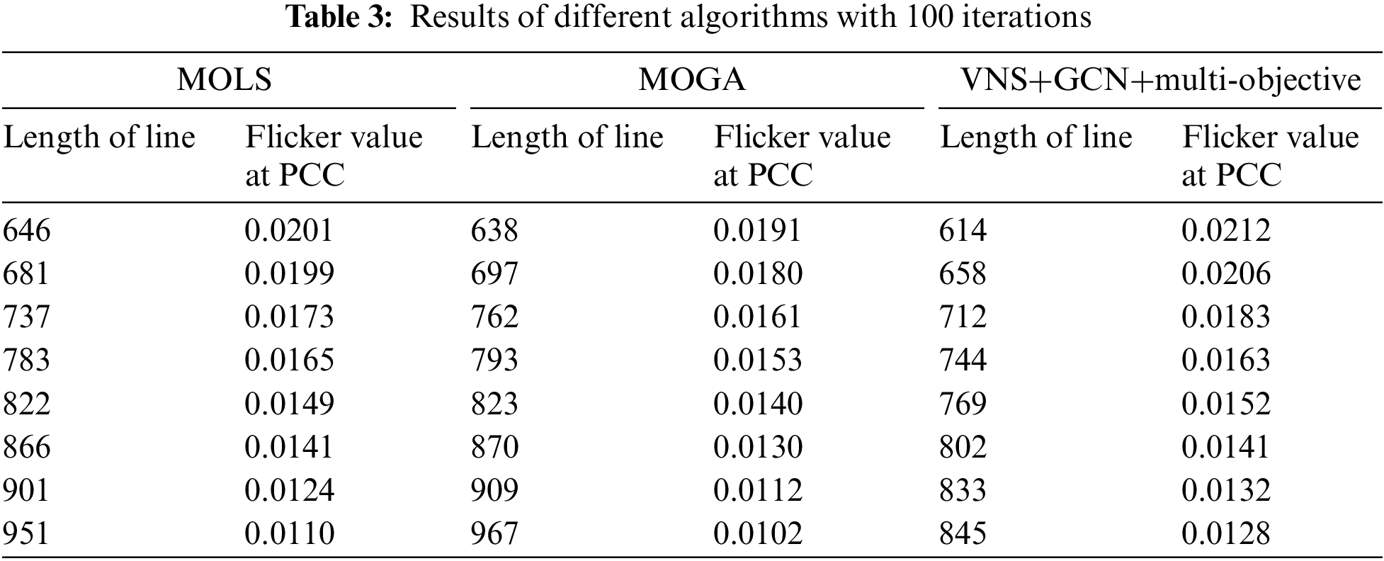
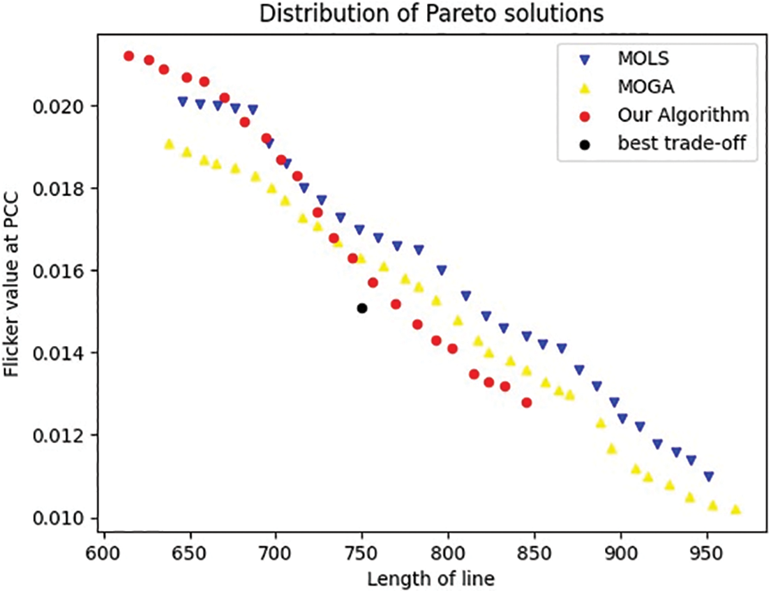
Figure 7: Distribution of Pareto solutions after 100 iterations of different algorithms

5.2 Ablation Study

To explore the role of each module in our proposed algorithm, we compared the PCC results obtained by three algorithms as well as the running speed: the original VNS algorithm, the VNS algorithm with multi-objective, and the VNS algorithm with GCN and multi-objective. It can also be seen from Tables 5 and 6 that the planning optimization based on the improved algorithm has faster convergence speed and better convergence performance. Fig. 8 clearly shows the superiority of our algorithm in ablation experiments.

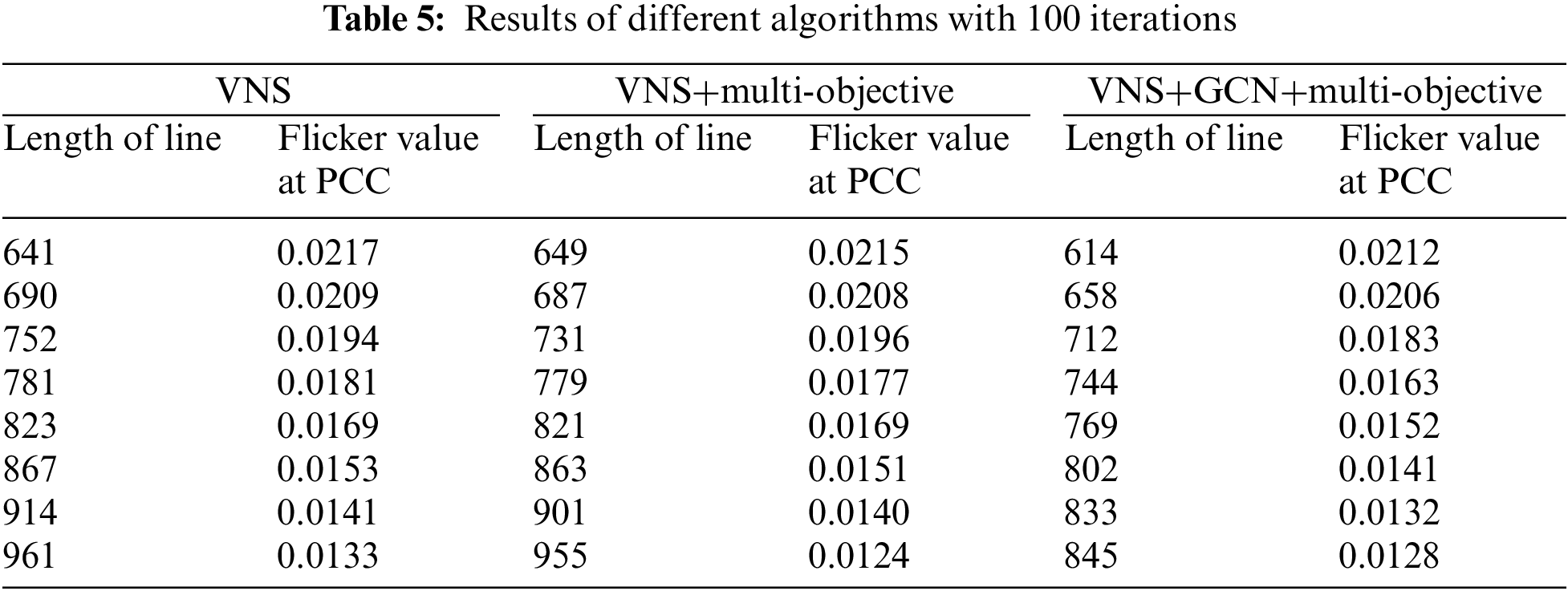
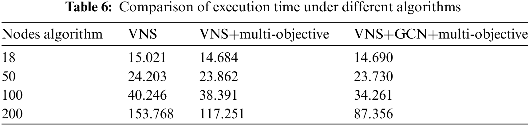
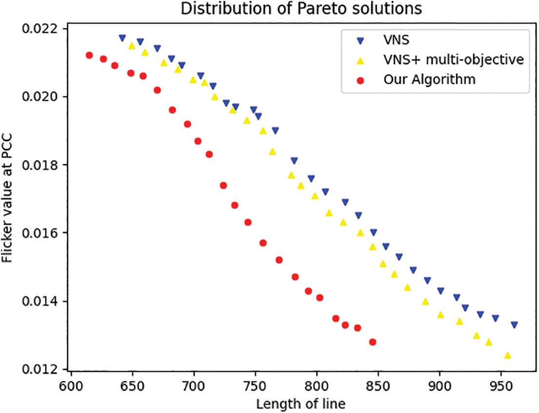
Figure 8: Distribution of Pareto solutions after 100 iterations of ablation study

6  Conclusion

An improved GNN Representation Learning and Multi-objective Variable Neighborhood Search Algorithm is proposed to solve the path network design problem of wind farms. The pre-processing of GCN improves the running speed and accuracy of the following algorithms. Meanwhile, the combination of the multi-objective algorithm and the variable neighborhood search algorithm improves the convergence of the algorithm, which is conducive to finding the optimal solution satisfying the multi-objective. While considering the PCC flicker value, the investment is minimized to ensure the power quality of the system. Our method has improved power quality by 6.1% compared to the latest algorithm and performance by 8.6% compared to the traditional VNS algorithm at a similar cost.

In our model, we focus on only two goals: economy and power quality. In fact, there are many more variables involved, such as the impact of the wind farm’s environment and the quality of components in the system. On the other hand, this paper improves the variable neighborhood search algorithm in two aspects, which increases the complexity and computation amount of the program. However, our method still has shortcomings. When GCN adds, deletes, or rearranges nodes in the graph, it needs to recalculate the representation of neighbor nodes, which leads to poor adaptability and long calculation time. Therefore, if GCN can be modified and set as an adaptive node, the calculation workload can be reduced. In addition, optimizing the neighborhood search algorithm is also one of our next research directions.

Acknowledgement: The support of all the members of the research group of CEPRI is especially acknowledged.

Funding Statement: This study was supported by the Natural Science Foundation of Zhejiang Province (LY19A020001).

Author Contributions: The authors confirm contribution to the paper as follows: study conception and design: Li Yingchao, Wang Jianbin and Wang Haibin; data collection: Li Yingchao, Wang Jianbin and Wang Haibin; analysis and interpretation of results: Li Yingchao and Wang Jianbin; draft manuscript preparation: Li Yingchao and Wang Haibin. All authors reviewed the results and approved the final version of the manuscript.

Availability of Data and Materials: Data supporting this study are included within the article.

Conflicts of Interest: The authors declare that they have no conflicts of interest to report regarding the present study.

References

1. Yang, K., Kwak, G., Cho, K., Huh, J. (2019). Wind farm layout optimization for wake effect uniformity. Energy, 183, 983–995. [Google Scholar]

2. Veers, P., Dykes, K., Lantz, E., Barth, S., Bottasso, C. L. et al. (2019). Grand challenges in the science of wind energy. Science, 366(6464), eaau2027. [Google Scholar] [PubMed]

3. Sorkhabi, S. Y. D., Romero, D. A., Beck, J. C., Amon, C. H. (2018). Constrained multi-objective wind farm layout optimization: Novel constraint handling approach based on constraint programming. Renewable Energy, 126, 341–353. [Google Scholar]

4. Ju, X., Liu, F., Wang, L., Lee, W. J. (2019). Wind farm layout optimization based on support vector regression guided genetic algorithm with consideration of participation among landowners. Energy Conversion and Management, 196, 1267–1281. [Google Scholar]

5. Yang, K., Cho, K. (2019). Simulated annealing algorithm for wind farm layout optimization: A benchmark study. Energies, 12(23), 4403. [Google Scholar]

6. Reddy, S. R. (2020). Wind farm layout optimization (WindFLOAn advanced framework for fast wind farm analysis and optimization. Applied Energy, 269, 115090. [Google Scholar]

7. Moreno, S. R., Pierezan, J., dos Santos Coelho, L., Mariani, V. C. (2021). Multi-objective lightning search algorithm applied to wind farm layout optimization. Energy, 216, 119214. [Google Scholar]

8. Verma, M., Ghritlahre, H. K., Chaurasiya, P. K., Ahmed, S., Bajpai, S. (2021). Optimization of wind power plant sizing and placement by the application of multi-objective genetic algorithm (GA) in Madhya Pradesh, India. Sustainable Computing: Informatics and Systems, 32, 100606. [Google Scholar]

9. Dhoot, A., Antonini, E. G., Romero, D. A., Amon, C. H. (2021). Optimizing wind farms layouts for maximum energy production using probabilistic inference: Benchmarking reveals superior computational efficiency and scalability. Energy, 223, 120035. [Google Scholar]

10. Cazzaro, D., Pisinger, D. (2022). Variable neighborhood search for large offshore wind farm layout optimization. Computers & Operations Research, 138, 105588. [Google Scholar]

11. Rizk-Allah, R. M., Hassanien, A. E. (2023). A hybrid equilibrium algorithm and pattern search technique for wind farm layout optimization problem. ISA Transactions, 132, 402–418. [Google Scholar] [PubMed]

12. Xiao, H., Liu, Y., Liu, H. (2011). Comparison of two calculation methods of flicker caused by wind power. Asia-Pacific Power and Energy Engineering Conference, pp. 1–4. Wuhan, China. [Google Scholar]

13. Redondo, K., Gutiérrez, J. J., Azcarate, I., Saiz, P., Leturiondo, L. A. et al. (2019). Experimental study of the summation of flicker caused by wind turbines. Energies, 12(12), 2404. [Google Scholar]

14. Wang, B., Yang, D., Cai, G. (2020). Dynamic frequency constraint unit commitment in large-scale wind power grid connection. Power System Technology, 44(7), 2513–2519. [Google Scholar]

15. Chakroborty, P., Wivedi, T. (2002). Optimal route network design for transit systems using genetic algorithms. Engineering Optimization, 34(1), 83–100. [Google Scholar]

16. Ren, Y., Zhang, C., Zhao, F., Triebe, M. J., Meng, L. (2018). An MCDM-based multiobjective general variable neighborhood search approach for disassembly line balancing problem. IEEE Transactions on Systems, Man, and Cybernetics: Systems, 50(10), 3770–3783. [Google Scholar]

17. Zhang, Z., Wang, K., Zhu, L., Wang, Y. (2017). A Pareto improved artificial fish swarm algorithm for solving a multi-objective fuzzy disassembly line balancing problem. Expert Systems with Applications, 86, 165–176. [Google Scholar]

18. Ma, X., Zhang, Q., Tian, G., Yang, J., Zhu, Z. (2017). On Tchebycheff decomposition approaches for multiobjective evolutionary optimization. IEEE Transactions on Evolutionary Computation, 22(2), 226–244. [Google Scholar]

19. Wang, J., Su, Y., Lin, Q., Ma, L., Gong, D. et al. (2020). A survey of decomposition approaches in multiobjective evolutionary algorithms. Neurocomputing, 408, 308–330. [Google Scholar]

20. Abdelsalam, A. M., El-Shorbagy, M. A. (2018). Optimization of wind turbines siting in a wind farm using genetic algorithm based local search. Renewable Energy, 123, 748–755. [Google Scholar]

21. Stanley, A. P., Roberts, O., King, J., Bay, C. J. (2021). Objective and algorithm considerations when optimizing the number and placement of turbines in a wind power plant. Wind Energy Science, 6(5), 1143–1167. [Google Scholar]