Multi-Time Scale Optimal Scheduling of a Photovoltaic Energy Storage Building System Based on Model Predictive Control

Nomenclature

1  Introduction

Given the “double carbon” policy proposed by China to reach its carbon peak in 2030 and carbon neutrality in 2060, a new type of power system based on renewable energy will be constructed to promote green and low-carbon development [1,2]. Given this premise, the construction industry is under increasing pressure to improve its energy management and environmental protection efforts. As an industry that consumes a considerable amount of energy and resources, the mitigation measures taken by the construction industry offer huge potential for improving energy utilization, energy conservation, and emission reduction. One such measure is the development of photovoltaic storage building systems, an emerging renewable energy technology that combines solar panels, battery energy storage systems, and building energy management systems [3].

However, the photovoltaic storage building system still faces many problems in terms of practical application, one of which is system scheduling optimization. How to effectively dispatch solar panels, energy storage systems, and building energy management systems in photovoltaic storage building systems to achieve efficient energy use and optimize building energy consumption is an urgent problem in this field [4].

In view of this, reference [5] described the use of a building optimization dispatching model, including vehicle-to-building smart charging piles and temperature-controlled and other types of adjustable loads to achieve energy savings and emission reduction goals as low-carbon buildings. Reference [6] proposed a double-layer intelligent-building group energy management method that uses the shared characteristics of electric vehicle (EV) mobile energy storage to optimize energy complementarity. Reference [7] introduced a distributed scheduling strategy based on the alternating direction multiplier method to solve the day-ahead economic operation problem of building groups. Reference [8] developed a day-ahead economic optimization scheduling strategy for building clusters by constructing an energy trading framework centered on the operators of smart building clusters equipped with energy storage systems. Reference [9] proposed an energy management framework for smart building clusters with peer-to-peer power sharing as the core, and the optimal strategy for smart building clusters day-ahead operation is obtained by solving the fast alternating direction multiplier method. Reference [10] took demand-side resource utilization into consideration and conducts research on integrated energy day-ahead optimization scheduling in smart communities that combines the energy supply side and the user side. Thus, the above mentioned studies focus on optimizing the energy dispatch in various buildings using day-ahead dispatch optimization strategies, without considering the error of source load prediction, resulting in a system operation that is not the optimal case.

The multi-time scale energy optimization strategy can predict the source load and optimize the system energy scheduling under different time scales, which greatly reduces the difference between the scheduling plan and the actual scheduling caused by the prediction error. Reference [11] proposed a multi-time scale optimal scheduling model for regional integrated energy systems with high percentage of PV penetration to balance the cost of risk due to new energy uncertainty under different risk attitudes. Reference [12] proposed a three-stage energy management strategy for EV photovoltaic charging stations in residential quarters to reduce operating costs and narrow the peak-to-valley difference of the power grid. Reference [13] proposed a multi-time scale optimal scheduling strategy for electric bus charging stations equipped with photovoltaics that takes into account the cost of power battery losses, which reduces the peak-to-valley difference of the distribution network load on the basis of improving the operating economy of the bus company. Reference [14] proposed an intelligent building energy management strategy based on MPC to improve control performance in a time-varying environment with predictive data uncertainty. However, the abovementioned literature does not fully explore the potential of dispatchable loads as demand response resources nor consider the impact of disorderly charging of EV loads on the power grid.

Here, in order to address the fluctuations in system operation due to source-load prediction errors and the impact of EVs on the energy management system, and to fully utilize the ability of dispatchable loads as demand response resources, this paper proposes a multi-time scale optimal scheduling strategy for photovoltaic energy storage building system based on MPC. This strategy optimizes the load for both EVs and air conditioning (AC), reducing the effects of inaccurate source-load forecasting. Our proposed strategy was analyzed under different scenarios to determine its effectiveness with respect to the economy, stability, and photovoltaic consumption rate of the photovoltaic storage building system.

2  Photovoltaic Storage Building System Structure

The structure of the photovoltaic storage building system is shown in Fig. 1. It mainly includes the upper-level power grid, photovoltaic power generation units, energy storage units, and building loads. The building loads are divided into rigid loads, such as lighting and equipment loads, and flexible loads such as EV charging loads and AC loads. The system is equipped with a building energy management system that communicates with an upper-level power grid to obtain tariff information released by the grid. The energy management system can predict the power generation of photovoltaic power-generating units, the power of various types of loads in the building, and the number of EVs arriving at the building according to a set prediction time domain to optimize the building load according to the prediction value in accordance with a set of optimization objectives. Decisions can then be made regarding the output of photovoltaic power-generating equipment and energy storage equipment, as well as the amount of electricity to be exchanged with the upper-level power grid.

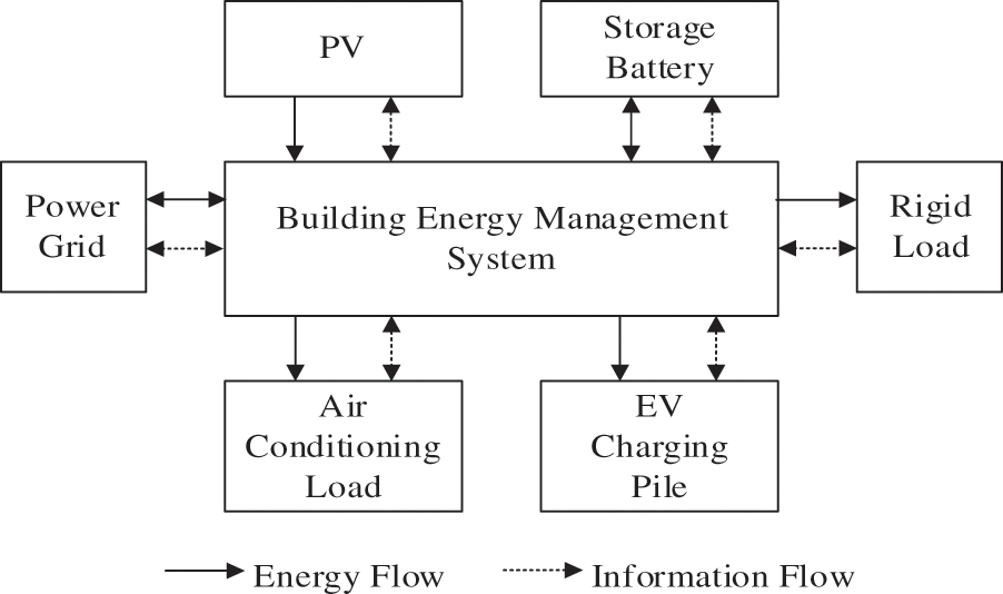
Figure 1: Photovoltaic storage building system structure diagram

For the AC load, the building can adjust the indoor temperature, and its internal energy management center can uniformly set the temperature of each room in the building and control the operating status of the AC. For the EV load, when the EV is connected to the charging pile in the building area, the built-in monitoring device of the charging pile records the access time, charging power, and departure time of the EV. According to the charging demand and vehicle information, the building energy scheduling center will conduct a unified dispatch of the charging piles connected to the EV load.

3  Building System Model

3.1 Building Photovoltaic Module Model

The rated power of photovoltaic power generation devices installed on buildings is usually taken as a fixed value. The actual output power is mainly related to the intensity of sunlight and the temperature of the photovoltaic panels, expressed as follows:

PPV(t)=PPV,NI(t)ISTC[1+Kp(T(t)−TSTC)](1)

where PPV(t) represents the photovoltaic power generation at time t, PPV,N is the photovoltaic device rated output power, I(t) is the solar light intensity at time t, ISTC is the standard test environment solar light intensity, Kp is the power temperature coefficient, T(t) is the photovoltaic solar panel surface temperature at time t, and TSTC is the standard test environment temperature.

3.2 Battery Model

As lithium-ion batteries have high energy density, high cycle life, low self-discharge rate and fast response capability, and with the continuous improvement of lithium-ion battery technology, its cost is also decreasing. Therefore, the lithium-ion battery is used as the supporting equipment for photovoltaic power generation. Its charging and discharging model is represented by the following:

{S(t+1)=S(t)+λchPESS,ch(t)Δt−PESS,dis(t)Δt/λdis0≤PESS,ch(t)≤UESS,ch(t)PESS,ch,max0≤PESS,dis(t)≤UESS,dis(t)PESS,dis,maxUESS,ch(t)+UESS,dis(t)≤1UESS,ch(t)∈{0,1},UESS,dis(t)∈{0,1}S(0)=S(T)(2)

where PESS,ch(t), PESS,dis(t) represent the charging and discharging power of the battery at time t, respectively; λch, λdis represent the charging and discharging efficiency of the battery, respectively; PESS,ch,max, PESS,dis,max denote the upper limit of the charging and discharging power of the battery, respectively; S(t) represents the energy stored in the battery at time t; UESS,ch(t), UESS,dis(t) are the charging and discharging state variable of the battery at time t, respectively; S(0), S(T) represent the energy stored in the battery at the beginning of the system and the end of the system, respectively; and Δt represents the time step.

3.3 Load Model

The building loads are divided into rigid loads and flexible loads. Flexible loads include AC loads and EV charging pile loads.

3.3.1 AC Load Model

In this paper, fixed-frequency AC is considered to participate in the regulation, and the electric power consumption of the AC is adjusted by changing the temperature setting value. Consider cooling in the summer as an example, in which the user sets the preferred temperature value to Tset, and the room temperature is maintained between [Tset−δ,Tset+δ]. The operation model of the AC can then be expressed as follows:

SAC(t)={1,Tin(t)≥Tset+δ0,Tin(t)≤Tset−δSAC(t−1),Tset−δ≤Tin(t)≤Tset+δ(3)

where SAC(t) is the running state of the air conditioner at time t, in which the value of 1 indicates that it is working, and the value of 0 indicates that it has stopped working; SAC(t−1) is the running state of the AC at time t − 1; and Tin(t) is the temperature of the room at time t.

In actual situations, when the fixed-frequency AC is working, it operates at the rated power state in which the operating state of the AC is only related to the temperature value set by the user. Its real-time power is given by

PAC(t)=PAC,NSAC(t)(4)

where PAC(t) is the operating power of the fixed-frequency AC at time t and PAC,N is the rated power of the fixed-frequency AC.

The cooling capacity provided by the AC at time t is as follows:

Qair(t)=ηACPAC(t)(5)

where ηAC is the energy efficiency ratio of the AC and Qair(t) is the cooling capacity of the AC at time t.

Room temperature variation is modeled using a first-order equivalent thermal parameter model, as given by

Tin(t+1)=Tout(t+1)−Qair(t)Req−[Tout(t)−Qair(t)Req−Tin(t)]e−ΔtReqCeq(6)

where Tout(t+1) is the outdoor temperature at time t + 1, Req is the equivalent thermal resistance of the AC room, Ceq is the equivalent heat capacity of the AC room, and Δt is the time step of the AC operation.

Optimizing the power consumption of the AC load is bound to have an impact on the user’s power consumption comfort. In this paper, temperature satisfaction is employed to describe user satisfaction with AC load participation in the demand response. The predicted mean vote (PMV) index, an indication of temperature satisfaction, represents the temperature at which most people feel comfortable in a certain environment [15], as represented by the following [16]:

IPMV=2.43−3.76(Ta−Tin)Mo(Icl+0.1)(7)

where Ta is the skin temperature, the value of which is 33.5 in this study; Mo is the metabolic rate of the human body, taken as 70.6 in this study; and Icl is the thermal resistance of the clothes worn by the user, which is assigned a value of 0.067 in this study.

From reference [17], the relationship between the PMV index value and human body comfort is shown in Table 1, which is divided into seven scenarios. When IPMV = 0, the human body feels the most comfortable. The optimal value in ISO-7730 is between −0.5 and 0.5 [17], and that in China is between −1 and 1 [18].

According to Eq. (7), when IPMV = 0, the indoor temperature is Tset. When IPMV = −1, 1, the indoor temperature is Tmin, Tmax, respectively.

In the day-ahead scheduling stage, the AC load adopts the most comfortable temperature control method, that is IPMV=0. In the intraday stage, to stabilize the source load prediction error, the AC load can fluctuate slightly based on the day-ahead scheduling results, but it needs to be between Tmin and Tmax.

3.3.2 Electric Vehicle Load Model

It is assumed that when the EV is parked at the charging pile in the building, the charging behavior of the EV is controlled by the building. The charging method before optimization is parking charging, that is, charging starts when the charging pile is connected after arriving at the building, and the charging process remains uninterrupted until the charging requirements are met and charging stops.

In contrast, the optimized charging control method uses sequential charging, in which the scheduling process is divided into multiple time periods of equal length. When the EV is connected to the charging pile, it will not be charged immediately. Instead, the charging start time is determined according to the optimization goal.

Assuming that there are n EVs in the building range, the matrix expression for the EV charging state variable at time t is

U(t)=[u1(t),u2(t),u3(t),⋯un(t)]1×n(8)

where U(t) is the charging state variable matrix of n EVs at time t; ui(t) is the charging state variable of the i-th EV at time t, in which ui(t)∈{0,1}, with a value of 0 indicating that the EV is not charging at time t and a value of 1 indicating that the EV is charging at time t.

The expression of the charge state variable matrix of n EVs over the whole dispatch period is

U=[u1(1)u2(1)⋯un(1)u1(2)u2(2)⋯un(2)⋮⋮⋱⋮u1(NT)u2(NT)⋯un(NT)](9)

If the charging power of the i-th EV is Pi,EV,N, then the charging power matrix of n EVs in the entire dispatch period is expressed as

PEV=[u1(1)P1,EV(1)u2(1)P2,EV(1)⋯un(1)Pn,EV(1)u1(2)P1,EV(2)u2(2)P2,EV(2)⋯un(2)Pn,EV(2)⋮⋮⋱⋮u1(NT)P1,EV(NT)u2(NT)P2,EV(NT)⋯un(NT)Pn,EV(NT)](10)

According to Eq. (10), it can be concluded that the charging power of the EV at time t in the dispatch period is

PEV,all(t)=∑i=1nui(t)Pi,EV(t),t=1,2,⋯,NT(11)

In this charging process, the charging state variable of the EV should be 0 before arriving at the building and after leaving the building, as given in the following:

{ui(t)=0,t<tstartui(t)=0,t>tend(12)

where tstart is the time when the EV arrives at the building and tend is the time when the EV leaves the building.

To ensure the power consumption satisfaction of EV users, it is necessary to satisfy the EV’s electric power to meet the user’s expectation when the user leaves the building. In addition, the charging process of EVs is modeled with the battery charging process.

4  Building Scheduling Optimization Model Based on Model Predictive Control

The multi-time scale scheduling process of the photovoltaic storage building system described in this paper is shown in Fig. 2.

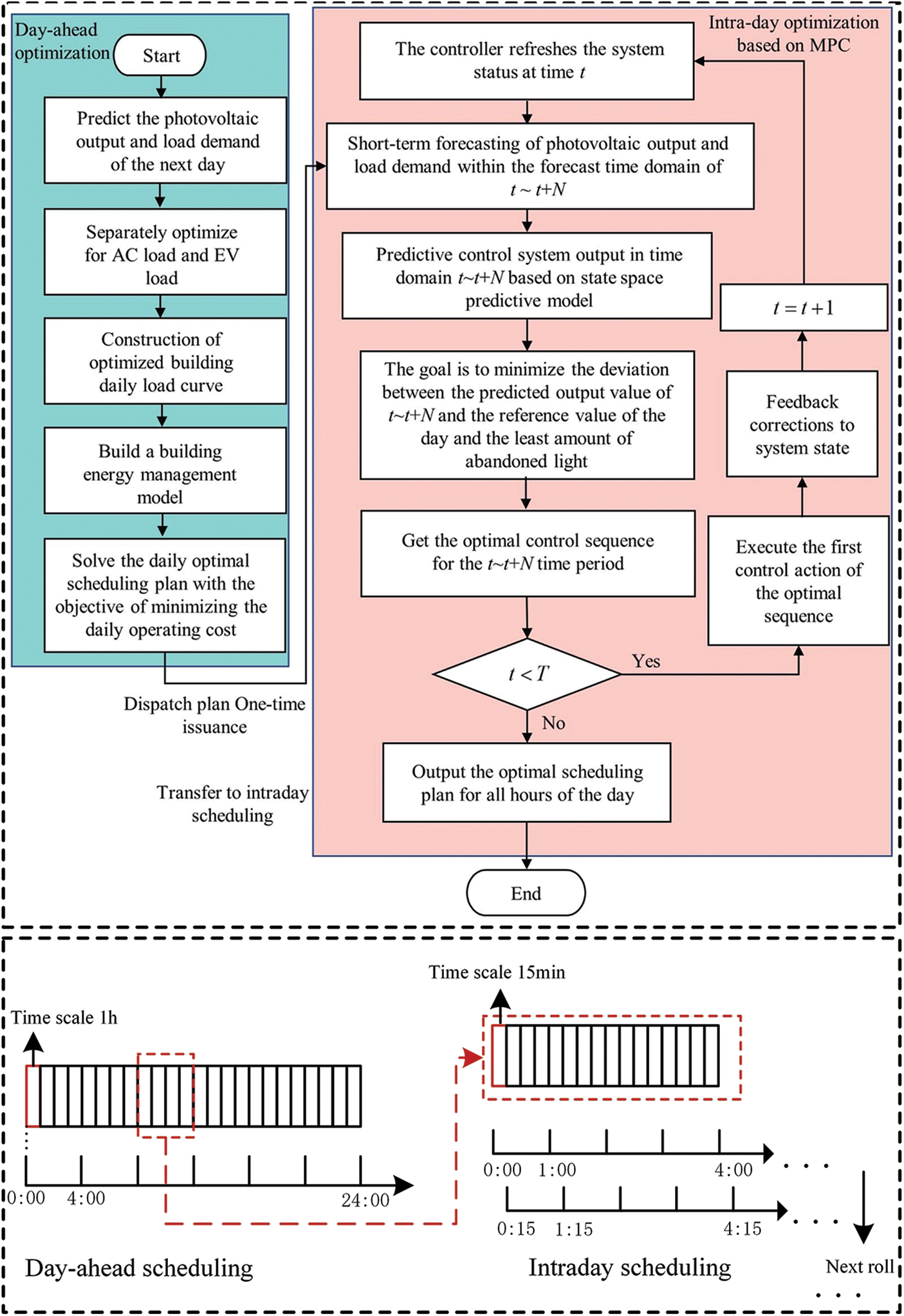
Figure 2: Multi-time scale energy management flow chart

In the day-ahead optimization stage, the scheduling cycle is 24 h, and the control time step is 1 h. The photovoltaic output and load demand of the next day are predicted, and the AC load and EV load are optimized according to the load optimization strategy described earlier. The building energy management model is then constructed, and the optimal day-ahead scheduling plan is solved with the goal of minimizing the cost to prepare for the intraday scheduling.

In the intraday optimization stage, rolling optimization of the MPC is used to continuously adjust and correct the day-ahead scheduling plan. The specific steps are as follows. The scheduling plan is formulated 4 h in advance, the control time step is 15 min, the length of the scheduling zone is 4 h, and the photovoltaic and load are re-predicted every 15 min. When t time according to the intraday scheduling model to get the time period for t to t + 4 h of the best scheduling program, only t time after the implementation of a time step that is t + 1 time after the results and the day-ahead scheduling plan is corrected. This process is then repeated based on the new forecast data until the 24-h intraday scheduling plan is completed.

4.1 Day-Ahead Optimal Scheduling Strategy

4.1.1 Objective Function

The goal of day-ahead scheduling optimization is to minimize the total cost within the scheduling cycle, including the cost of purchasing electricity from the grid, the revenue from selling electricity to the grid, the operation and maintenance costs of photovoltaic power generation equipment, and the operation and maintenance costs of batteries, as given by

minCtotal,a=Cbuy,a−Csale,a+CPV,a+CESS,a(13)

{Cbuy,a=∑t=1NT,aλbuy,a(t)Pbuy,a(t)ΔtCsale,a=∑t=1NT,aλsale,a(t)Psale,a(t)ΔtCPV,a=∑t=1NT,aKPVPPV,a(t)ΔtCESS,a=∑t=1NT,aKESS[PESS,dis,a(t)+PESS,ch,a(t)]Δt(14)

where NT,a is the number of steps in the day-ahead scheduling cycle, Cbuy,a is the cost of purchasing electricity from the grid in the day-ahead, Csale,a is the income from selling electricity to the grid in the day-ahead, CPV,a is the operation and maintenance cost of photovoltaic power generation equipment in the day-ahead, CESS,a is the operation and maintenance cost of the storage battery in the day-ahead, λbuy,a(t) is the electricity purchase price from the grid at time t, λsale,a(t) is the price of electricity sold to the grid at time t, Pbuy,a(t) is the power purchased from the grid at time t, Psale,a(t) is the power sold to the grid at time t, KPV is the operation and maintenance coefficient of the photovoltaic power generation equipment, and KESS is the operation and maintenance coefficient of the storage battery.

4.1.2 Constraint Conditions

Constraint conditions are divided into equality constraints and inequality constraints, where equality constraints are power balance constraints, and inequality constraints are equipment constraints and tie line power constraints.

(1) Power balance constraint:

PAC,a(t)+PEV,a(t)+Pload,a(t)=PPV,a(t)+PESS,dis,a(t)+Pbuy,a(t)−Psale,a(t)−PESS,ch,a(t)(15)

where Pload,a(t) is the rigid load power at time t.

(2) Power balance constraint:

0≤PPV,a(t)≤PPV,a,max(t)(16)

where PPV,a,max(t) is the maximum output of the photovoltaics at time t; this paper takes the predicted value of photovoltaics as the maximum output.

(3) Power balance constraint:

{QESS,a(0)=20%QESS,max0≤PESS,dis,a(t)≤UESS,dis,a(t)PESS,dis,max0≤PESS,ch,a(t)≤UESS,ch,a(t)PESS,ch,maxUESS,ch,a(t)+UESS,dis,a(t)≤1UESS,ch,a(t)∈{0,1},UESS,dis,a(t)∈{0,1}(17)

where QESS,a(t) is the energy capacity value of the battery at time t; QESS,max is the maximum energy capacity value of the battery; UESS,dis,a(t), UESS,ch,a(t) are the state variables of battery discharge and charging at time t, taking values of 0 and 1, respectively; and PESS,ch,max, PESS,dis,max are the maximum charging and discharging power of the battery, respectively.

(4) Power balance constraint:

{0≤Pbuy,a(t)≤Ubuy,a(t)Pgrid,max0≤Psale,a(t)≤Usale,a(t)Pgrid,maxUbuy,a(t)+Usale,a(t)≤1Ubuy,a(t)∈{0,1},Usale,a(t)∈{0,1}(18)

where Pgrid,max is the maximum power value of the tie line; and Ubuy,a(t), Usale,a(t) are the state variables of electricity purchase and sales at time t, respectively, taking a value of 0 or 1.

4.2 Intraday Rolling Optimization Scheduling Strategy

The day-ahead scheduling calls the forecasted values of photovoltaics and loads on the previous day. The use of earlier forecasted values will inevitably lead to large error relative to the actual situation. Therefore, intraday scheduling needs to be based on new forecasts of photovoltaic power generation and various loads. With this approach, the lead time of the forecast in the intraday period is shortened, the forecast occurs 4 h in advance, and the minimum step size in the intraday optimization process is 15 min. Rolling optimization of the MPC is used to formulate the intraday scheduling strategy.

4.2.1 Objective Function

The purpose of intraday scheduling is to minimize the output deviation of each unit of the system caused by the day-ahead-intraday source load prediction error and absorb photovoltaic power generation to the maximum extent. Therefore, the optimal goal of intraday scheduling is to minimize the deviation in the charging and discharging power of the storage battery and the power of the tie line in the day-ahead-intraday, as well as to minimize the intraday light abandonment. Its objective function is given by

minCtotal,b=Cgrid,b+CESS,b+CPV,b(19)

{Cgrid,b=∑t=1NT,bωgrid[|Pbuy,b(t)−Pbuy,a(t)|+|Psale,b(t)−Psale,a(t)|]ΔtCESS,b=∑t=1NT,bωESS[|PESS,ch,b(t)−PESS,ch,a(t)|+|PESS,dis,b(t)−PESS,dis,a(t)|]ΔtCPV,b=∑t=1NT,bωPV[PPV,b,max(t)−PPV,b(t)]Δt(20)

where NT,b is the number of intraday scheduling cycle steps, Cgrid,b is the power offset penalty cost of the tie line in the day-ahead-intraday, CESS,b is the battery power offset penalty cost in the day-ahead-intraday, CPV,b is the intraday cost of abandoned light, ωgrid is the power offset penalty coefficient of the tie line in the day-ahead-intraday, ωESS is the penalty coefficient of the battery power offset in the day-ahead-intraday; and ωPV is the penalty coefficient for the intraday light abandonment.

4.2.2 Constraint Condition

The constraints are the same as the day-ahead constraints, including power balance, equipment, and electricity purchase and sale constraints. The difference is that compared with the day-ahead constraints, in the intraday rolling optimization process, the cycle of single optimal scheduling is 4 h. After obtaining the optimal scheduling plan for the time period from t to t + 4 h, only the result of a time step after time t, that is, time t + 1, is executed. The scheduling plan is then employed with a time period from t + 1 to t + 1 + 4 h, and the data before t + 1 follows the result of the previous scheduling period, that is, from t to t + 4 h. This is the coupling constraint of the time before and after the intraday equipment, expressed as

{PESS,ch,b(t)=PESS,ch,b′(t)PESS,dis,b(t)=PESS,dis,b′(t)Pbuy,b(t)=Pbuy,b′(t)Psale,b(t)=Psale,b′(t)(21)

where PESS,ch,b′(t), PESS,dis,b′(t), Pbuy,b′(t), Psale,b′(t) are the charging and discharging power of the battery and the power of purchasing and selling electricity from the grid at time t in the last scheduling cycle, respectively.

5  Case Analysis

5.1 Case Setting

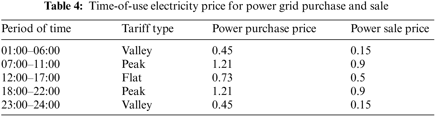
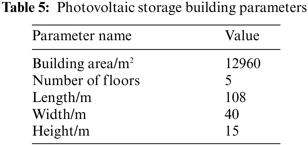
Taking a smart office building on a work day during the summer as an example, the system operation structure is shown in Fig. 1. In the case scenario, the photovoltaic capacity on the roof of the building is 300 kW, the photovoltaic operation and maintenance cost is 0.02 ¥/kWh, and the battery capacity is 500 kWh. The maximum charging and discharging power of the battery is 100 kW, the initial capacity of the battery is 150 kWh, and the operation and maintenance cost of the battery is 0.15 ¥/kWh. The outdoor temperature condition is shown in Fig. 3. The rigid load demand inside the building is shown in Fig. 4. There are 100 ACs in the building; the specific parameters of the ACs are shown in Table 2. There are 20 EV charging piles in the building; the EV parameters are listed in Table 3. The grid time-of-use electricity price is shown in Table 4. The photovoltaic storage building parameters is shown in Table 5.

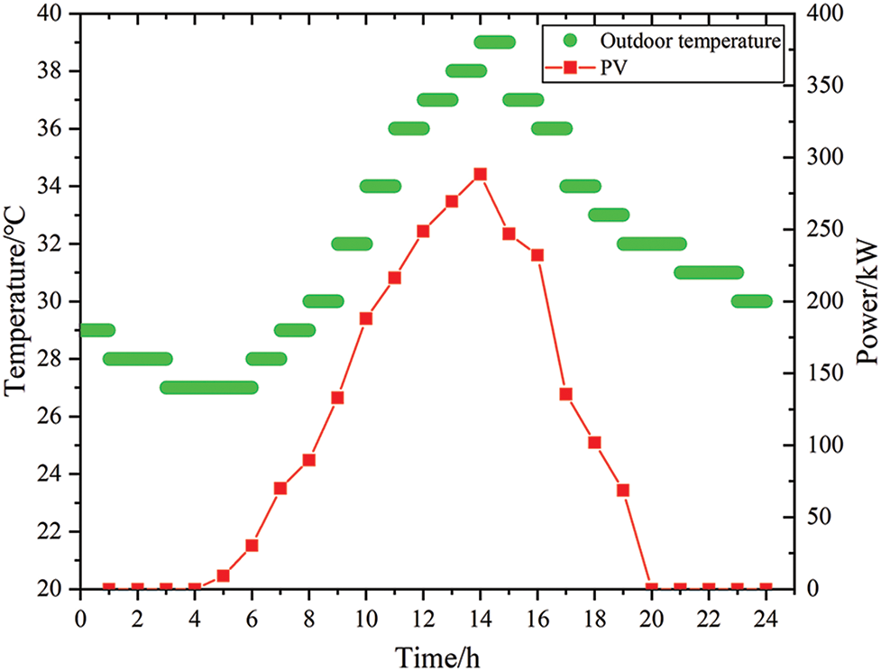
Figure 3: Building outdoor temperature and photovoltaic forecast results

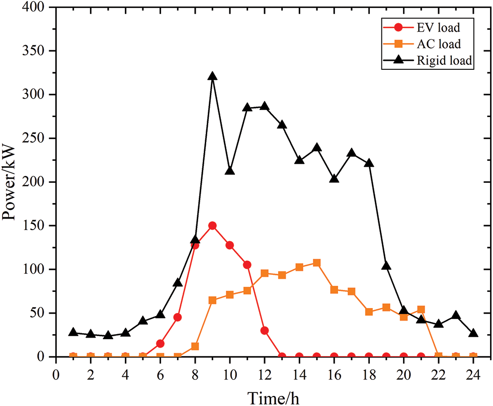
Figure 4: Load forecast results

5.2 Day-Ahead Scheduling Analysis

The outdoor temperature and photovoltaic forecast results of the building are shown in Fig. 3, and the load forecast results are presented in Fig. 4. The EV load and AC load were simulated according to the data described in the table. The peak charging load of EV charging piles in the building area is from 8:00–9:00, as this corresponds to the arrival time of building staff (Fig. 4). After an EV is parked, it is directly connected to the charging pile for charging; at this point, no reasonable load optimization has been performed. As for the AC load, the AC is turned on successively from around 8:00 (Fig. 4). The AC load increases gradually with the outdoor temperature. After 18:00, as the staff leave, the AC load gradually decreases until 22:00, when all the personnel have left, at which point the AC load decreases to 0.

(1) Day-ahead load optimization analysis

For the EV and AC loads, load optimization is carried out using the method described above. The optimized results are shown in Figs. 5 and 6.

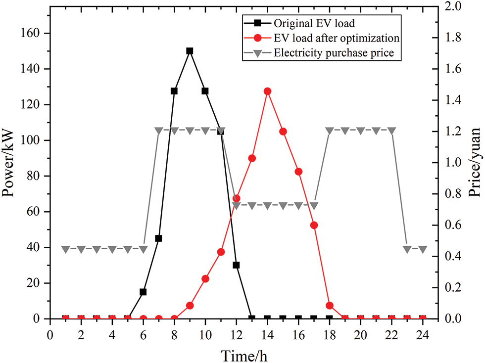
Figure 5: Electric vehicle load optimization results

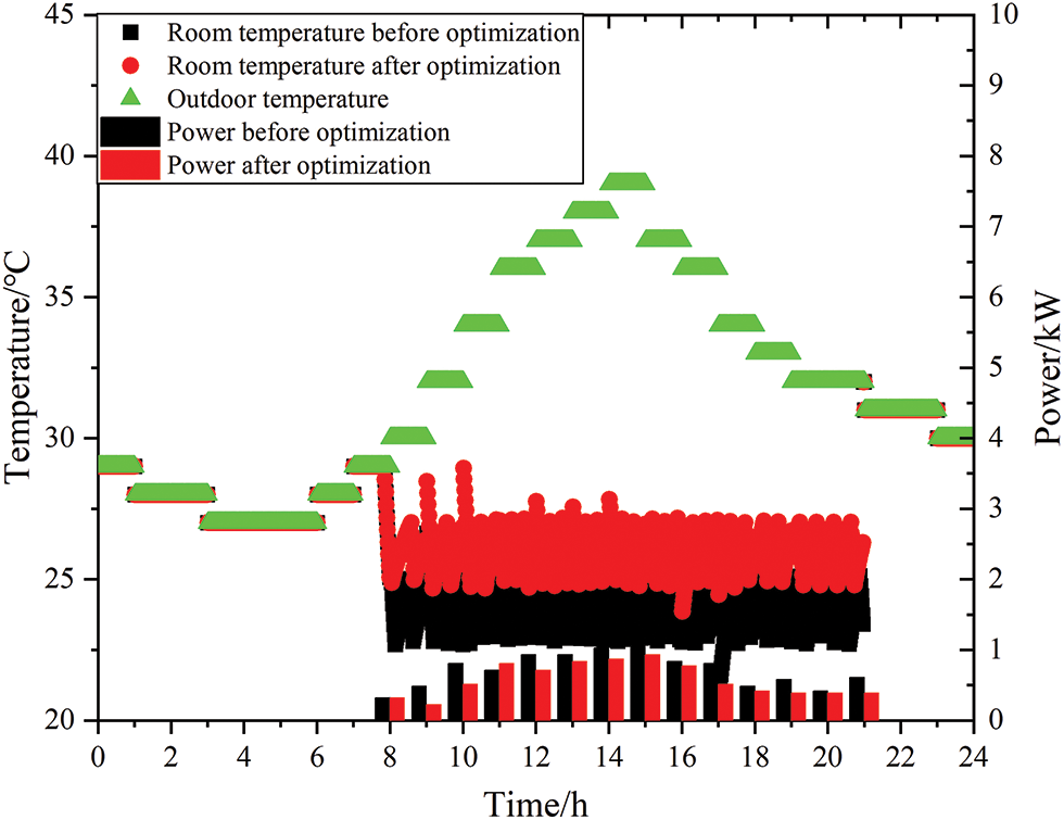
Figure 6: Air conditioner load optimization results

From Fig. 5, the EV load showed a significant shift over time. The peak load period changed from 8:00–11:00 to 12:00–17:00, and moved from the peak electricity price period to the normal electricity price period, which reduces the charging cost of EVs. The EV load remains unchanged in terms of the total amount, but the peak value decreases, which reduces the impact of the EV load on the building power supply system.

Fig. 6 shows that the overall AC load is in a state of load reduction. This is because the building can adjust the indoor temperature, and its internal energy management center uniformly sets the temperature of each room in the building and controls the operating status of the AC. Before optimization, the cooling temperature of the AC is set at about 24°C; after optimization, the cooling temperature of the AC is set at about 26°C.

The results of the total load optimization are shown in Fig. 7. The total load showed a trend of reduction in the peak period and a smoother load curve. The total load before and after optimization changed from 4,783.40 to 4,598.41 kW, a decrease of 184.99 kW, which is a 4.02% reduction; the cost dropped from 4,601.78 to 4,193.30 ¥, a decrease of 408.47 ¥, which is a 9.74% decrease; and the peak load changed from 534.72 to 440.34 kW, a reduction of 94.38 kW, which is a 21.43% decrease. Therefore, the load optimization strategy of the building can effectively optimize the load distribution, allowing for enhanced system stability and economy and reduced system load expenditure.

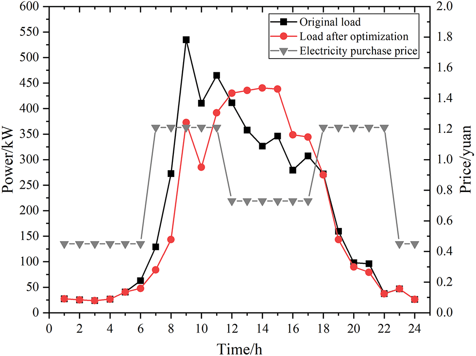
Figure 7: Total load optimization results

(2) Day-ahead scheduling plan analysis

The day-ahead scheduling plan of the system is obtained by reasonably scheduling each unit in the system according to the day-ahead objective function, that is, the minimum total system cost, as shown in Fig. 8. When the electricity price of the grid is at the valley price from 0:00 to 6:00, the system starts to purchase electricity from the grid and charge the battery. From 7:00 to 11:00, the power grid is at peak electricity price. To reduce the cost, the battery starts to discharge to the system, and all photovoltaics are consumed. When the electricity price of the grid is at the normal electricity price from 12:00 to 17:00, the battery starts to charge, because the charging and discharging costs of the battery and the cost of loss are less than the cost of purchasing electricity from the grid during the peak period of the electricity price. When the electricity price of the grid is at its peak from 18:00 to 22:00, the battery will be discharged first to supply power to the load. When the electricity price of the grid is at a valley price from 23:00 to 24:00, the battery is charged to supply the next day’s output.

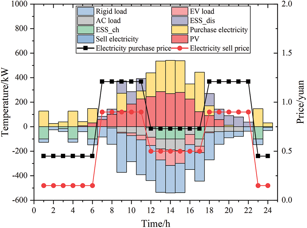
Figure 8: System day-ahead scheduling plan results

(3) Model validity analysis

To verify the effectiveness of the system scheduling control strategy, here, five scenarios are set up for comparative analysis in terms of economy and carbon emission reduction. The specific costs and carbon emission reductions of each scenario are listed in Table 6.

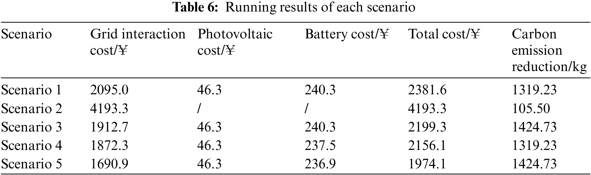
Scenario 1: The system contains photovoltaic and battery units, and load optimization is not considered.

Scenario 2: The system does not contain photovoltaic or battery units, and load optimization is considered.

Scenario 3: The system contains photovoltaic and battery units, and only AC load optimization is considered.

Scenario 4: The system contains photovoltaic and battery units, and only EV load optimization is considered.

Scenario 5: The system contains photovoltaic and battery units, and load optimization is considered.

From Table 6, the total operating cost of Scenario 5 within 1 day is the lowest, at 1,974.1 ¥, and the carbon emission reduction is the highest, at 1,424.73 kg. This represents a reduction of 407.5 ¥ in total system cost compared to Scenario 1, a decrease of 17.11%, and an increase in carbon emission reduction by 105.5 kg, which is an increase of 7.99%. This is because when load optimization is considered, the system will move the EV load from the high electricity price period to the low electricity price period, and adjust the output of the AC load according to the comfort of the human body, thus reducing costs and carbon emissions. Compared with Scenario 1, the total system cost of Scenario 2 increases by 1,811.7 ¥, which is an increase of 43.21%, and the carbon emission reduction decreases by 1,213.73 kg, which is a decrease of 92.00%. This is because there are no photovoltaics or battery units in Scenario 2; the system directly purchases electricity from the grid without using clean energy, and carbon reduction is achieved solely by load optimization. Compared with Scenario 4, the carbon emission reduction in Scenario 3 increases by 105.5 kg, which is an increase of 7.99%. This is because the charging amount of the EVs does not change during EV load optimization; only the charging time changes. Comprehensive analysis of the model proposed in this paper could reduce costs, improve system economy, reduce carbon emissions, and facilitate the construction of low-carbon building environments.

5.3 Intraday Scheduling Analysis

Before the intraday scheduling of the system, the short-term forecast for the photovoltaics and load within 1 day is carried out first. The random error of normal distribution is superimposed on the previous forecast results to simulate the short-term intraday forecast data [19,20]. Specifically,

{PPV,b,max(t)=PPV,a,max(t)[1+εPV(t)]Pload,b,max(t)=Pload,a,max(t)[1+εload(t)](22)

where εPV, εload are the forecast error deviation rates of the photovoltaics and load in the day-ahead-intraday, respectively.

The curves of short-term intraday photovoltaics and load forecasts obtained from Eq. (22) are shown in Fig. 9.

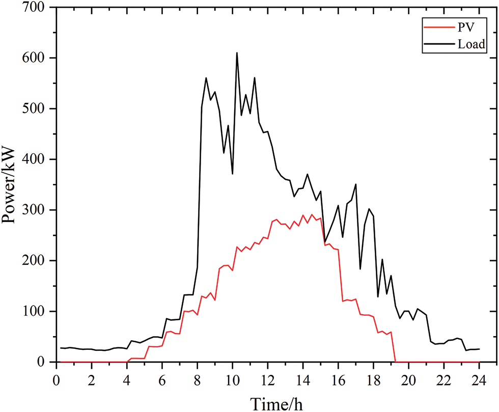
Figure 9: Intraday photovoltaic and load short-term forecast

(1) Analysis of intraday scheduling results

Based on the more accurate intraday short-term forecast, the system scheduling is optimized with a smaller time step to obtain the intraday scheduling results, as shown in Fig. 10. It can be seen that the minimum step size of the intraday scheduling strategy is 15 min, and the power of the entire system is balanced. Compared with the day-ahead scheduling, the output of each unit of the system does not change significantly in the intraday scheduling. Only a slight adjustment is made to eliminate the power deviation caused by the day-ahead-intraday source–load forecast error.

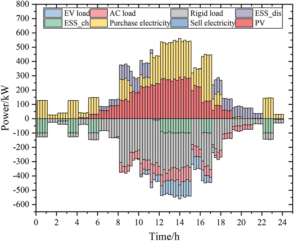
Figure 10: System intraday scheduling plan results

The day-ahead-intraday output deviation of the battery and the tie line in the system are shown in Figs. 11 and 12, respectively. The status flags of the battery’s day-ahead-intraday charge and discharge status have not changed; only the output values at each time point change slightly, making intraday adjustments less expensive. The battery does not undergo frequent charge and discharge state transitions, which slows down the loss of battery life. Regarding the output of the tie line, the intraday optimization results are basically consistent with the day-ahead, avoiding any impact of frequent purchase and sale of electricity, which is conducive to the stability of system operations.

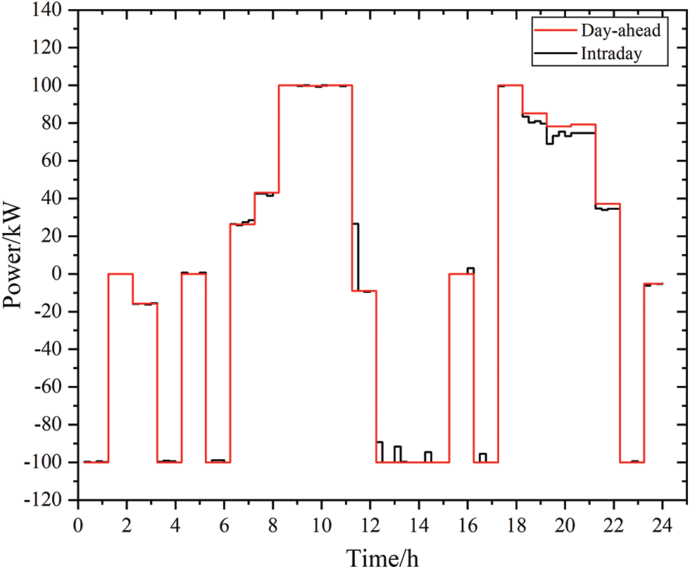
Figure 11: Battery day-ahead-intraday output deviation

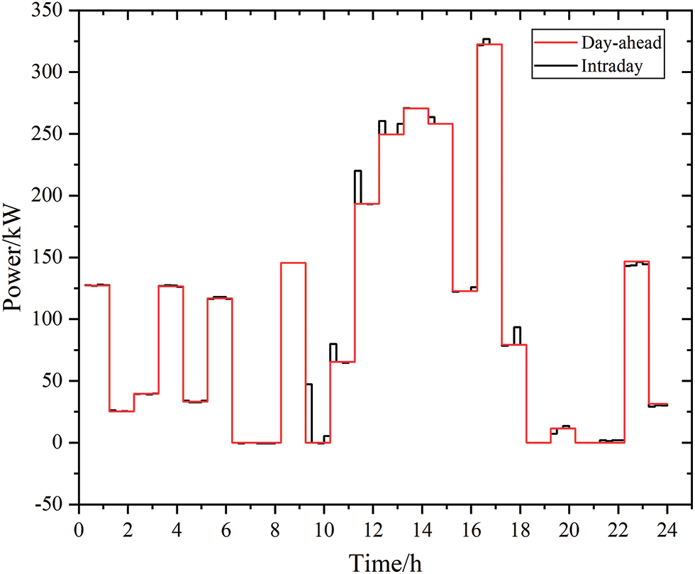
Figure 12: Day-ahead-intraday output deviation of the tie line

(2) Comparison of different control methods

To verify the smoothing effect of the MPC rolling optimization proposed in this paper on the fluctuation of the system tie line, three control methods are set up for comparative analysis. The output results of the tie line under the three control modes are shown in Fig. 13.

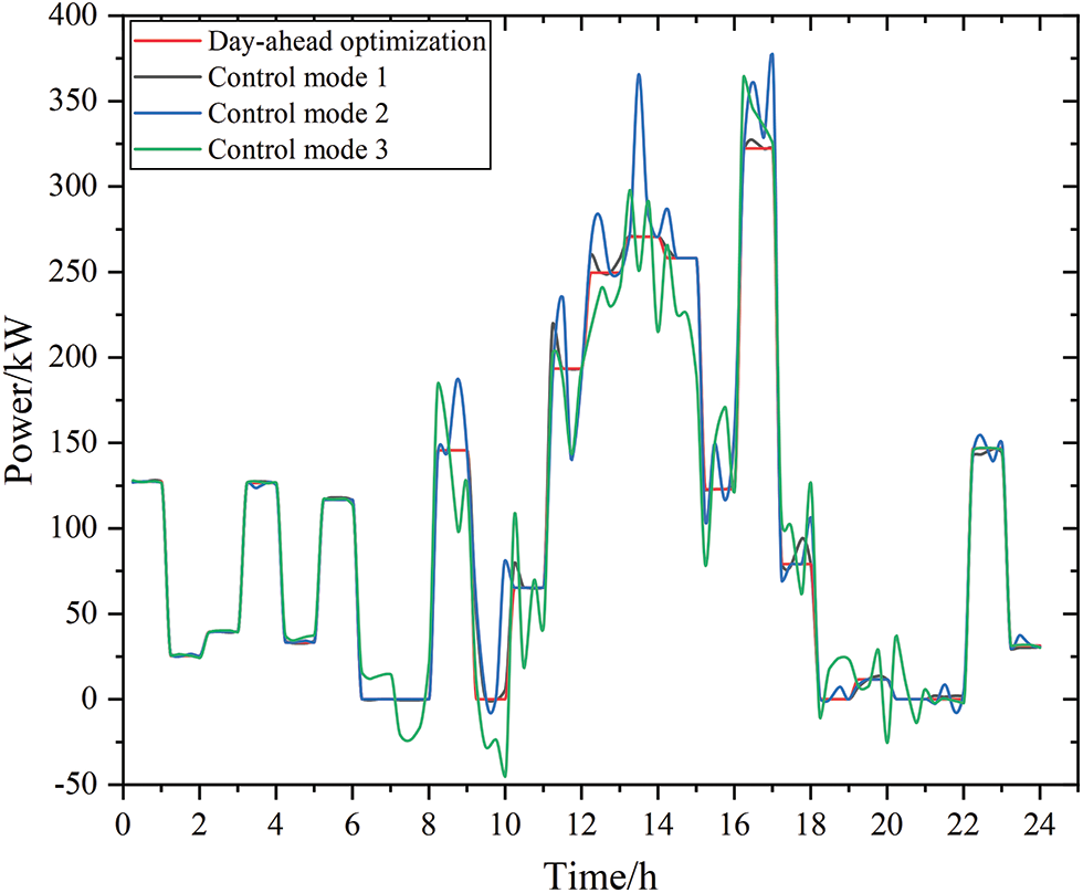
Figure 13: Diagram of the output results for the tie line under the three control modes

Method 1: Use the intraday MPC rolling optimization mentioned in this article.

Method 2: Intraday non-rolling optimization. That is, based on the intraday short-term forecast results, the intraday output plan for all time periods is solved, and all intraday scheduling plans are issued together to correct the day-ahead scheduling results.

Method 3: Execute the day-ahead scheduling optimization strategy during the intraday period, and for the deviation of the day-ahead-intraday source-load prediction, all the deviations are smoothed by the external grid through the contact line.

Fig. 13 shows that the MPC rolling optimization control method proposed in this paper is the most effective for stabilizing the fluctuation of the tie line. This is because the control method based on MPC rolling optimization will re-predict the source load every 15 min, has an optimal scheduling strategy within the scheduling cycle that is based on newer state predictions, and executes only the first control action within the cycle after obtaining the result of the scheduling optimization. This allows for more flexible, real-time adjustment of the state of the system, so as to better cope with the deviation of the output of the day-ahead-intraday contact line and reduce the impact of inaccurate source and load predictions.

In control method 2, the system calculates the intraday output plan for all time periods based on the intraday short-term forecast results and issues all intraday scheduling plans together. This control method only relies on a single optimization to adjust the state of the system. When late prediction error occurs, it cannot accurately stabilize the error, resulting in a sudden change in the power of the tie line.

In control method 3, the tie line power fluctuates greatly, and it is difficult to effectively track the day-ahead planned value. This is because, in this control method, the impact of the day-ahead-intraday source load prediction error is smoothed by the tie line, and other scheduling units in the system do not optimize scheduling.

(3) System photovoltaic consumption analysis

The model established in this paper considers the light abandonment penalty in the intraday stage to ensure that each unit of the system can track the day-ahead scheduling plan as accurately as possible, and at the same time adjust the power of the AC load in the intraday stage to maximize photovoltaic power generation consumption under the premise of satisfying the user comfort constraints and reducing the occurrence of light abandonment. To verify the superiority of the model proposed in this paper in terms of photovoltaic consumption, the following scenarios are established for comparative analysis.

Scenario 6: Consider day-ahead-intraday scheduling optimization, but the optimization goal of intraday scheduling only considers the output deviation penalty; it does not consider the light abandonment penalty.

Scenario 7: Consider day-ahead-intraday scheduling optimization; the goal of intraday scheduling optimization is consistent with this paper, but the AC load control method is consistent with the day-ahead.

Scenario 8: Application of the model proposed in this paper.

It can be seen from Table 7 that the photovoltaic consumption rate of the model proposed in this paper is as high as 98.57%, thus, using the proposed model (Scenario 8), the system is able to efficiently consume photovoltaic energy with consideration of the impact of the day-ahead-intraday source load prediction error. This is because the system can control the power of the AC load to stabilize system power fluctuations when the power of the intraday source load is unbalanced. In Scenario 6, the photovoltaic consumption rate decreased by 10.67% compared to Scenario 8. This is due to the fact that the objective function of intraday scheduling does not consider PV consumption; thus, when the actual PV power generation is higher than the day-ahead scheduling value during system optimization, the system will choose to abandon PVs to minimize deviation in the equipment output. In Scenario 7, the photovoltaic consumption rate decreased by 10.87% compared to Scenario 8. This is because the AC load control method is the same as the day-ahead and lacks the AC load regulation capability, when the actual PV power generation is higher than the day-ahead scheduling value, the system can only adjust the output of the battery or tie line or choose to abandon PVs.

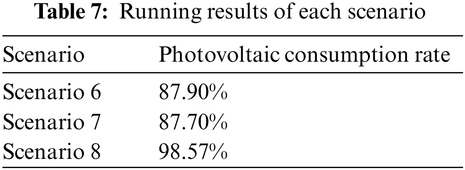
In summary, the model proposed in this paper can effectively improve the PV consumption capacity of the system, stabilize the equipment output fluctuations caused by the prediction error of the day-ahead-intraday source load, and improve the economy and robustness of the system.

6  Conclusion

To effectively optimize the operation of photovoltaic storage building systems, improve the energy consumption of the building, and realize the efficient use of energy, this paper proposes a multi-time scale optimal scheduling model for the system based on MPC. The following conclusions can be drawn from the cases/scenarios presented:

(1)   The load optimization strategy proposed in this paper has reduced the total operating cost of the photovoltaic storage building systems by 17.11% while increasing carbon emission reduction by 7.99%. This effectively enhances the economic and low-carbon performance of the system.

(2)   The MPC-based multi-time scale optimal scheduling strategy for the photovoltaic storage building system proposed in this paper can more flexibly adjust the state of photovoltaic storage building systems, reduce the impact of inaccurate source–load predictions, and enhance system operation stability.

(3)   The photovoltaic storage building system stabilizes system power fluctuations by controlling the power of the AC load, increasing the photovoltaic consumption rate by 10.87%, achieving a system photovoltaic consumption rate of 98.57%, and further enhancing the economic efficiency of the system.

Acknowledgement: None.

Funding Statement: The authors received no specific funding for this study.

Author Contributions: Study conception and design: Ximin Cao, Xinglong Chen, He Huang; data collection: He Huang, Qifan Huang, Yang Chen; analysis and interpretation of results: Xinglong Chen, He Huang; draft manuscript preparation: He Huang; review and editing: Ximin Cao, Yang Chen. All authors reviewed the results and approved the final version of the manuscript.

Availability of Data and Materials: The data presented in this study are available on request from the corresponding author. The data are not publicly available due to patent protection.

Conflicts of Interest: The authors declare that they have no conflicts of interest to report regarding the present study.

References

1. Li, H., Liu, D., Yao, D. (2021). Analysis and reflection on the development of power system towards the goal of carbon emission peak and carbon neutrality. Proceedings of the CSEE, 41(18), 6245–6258 (In Chinese). [Google Scholar]

2. Yun, B., Zhang, E., Zhang, G., Ma, K., Zhang, B. (2022). Optimal operation of an integrated energy system considering integrated demand response and a dual carbon mechanism. Power System Protection and Control, 50(22), 11–19. [Google Scholar]

3. Wang, L., Gao, H., Liu, C., Cai, W., Hu, M. et al. (2022). Electricity carbon coupling sharing among intelligent buildings considering time-of-use carbon emission measurement. Power System Technology, 46(6), 2054–2063. [Google Scholar]

4. Wei, W., Skye, H. M. (2021). Residential net-zero energy buildings: Review and perspective. Renewable and Sustainable Energy Reviews, 142, 110859. https://doi.org/10.1016/j.rser.2021.110859 [Google Scholar] [PubMed] [CrossRef]

5. Yu, S., Du, Y., Shi, Y., Su, H., Feng, D. et al. (2021). Optimal scheduling of low-carbon building considering V2B smart charging pile groups. Electric Power Automation Equipment, 41(9), 95–101. [Google Scholar]

6. Hu, H., Ai, X., Hu, J., Wang, K. (2022). Energy management method of smart building cluster considering mobile energy storage characteristics of electric vehicles. Electric Power Automation Equipment, 42(10), 227–235. [Google Scholar]

7. Yang, Z., Ai, X. (2020). Distributed optimal scheduling for integrated energy building clusters considering energy sharing. Power System Technology, 44(10), 3769–3776. [Google Scholar]

8. Hu, J., Li, P., Lin, S., Ding, J. (2021). Energy-sharing method for smart building clusters considering differences of time-of-use prices and based on master-slave game. Power System Technology, 45(12), 4738–4748. [Google Scholar]

9. Zhou, J., Li, J., Ma, H., Jiang, D., Zhang, H. (2021). Distributed optimal scheduling for smart building clusters considering peer-to-peer electric energy sharing. Electric Power Automation Equipment, 41(10), 113–121. [Google Scholar]

10. Cai, Z., Peng, M., Shen, M. (2021). Day-ahead optimal scheduling of smart integrated energy communities considering demand-side resources. Electric Power Automation Equipment, 41(3), 18–24+32 (In Chinese). [Google Scholar]

11. Wang, C., Sun, J., Xu, Q., Ge, J. (2023). Optimal scheduling based on the CVaR method for regional integrated energy system with high proportion photovoltaic. Advanced Engineering Sciences, 55(2), 97–106. [Google Scholar]

12. Wei, J., Liu, Q. (2017). Tri-period energy management strategy for PV-assisted EV charging station in residential area. Electric Power Automation Equipment, 37(8), 249–255. [Google Scholar]

13. Chen, L., Qin, M., Gu, S., Qian, K., Xu, X. (2020). Optimal dispatching strategy of electric bus participating in vehicle-to-grid considering battery loss. Automation of Electric Power Systems, 44(11), 52–60. [Google Scholar]

14. Jin, X., Jiang, T., Mu, Y., Long, C., Li, X. et al. (2019). Scheduling distributed energy resources and smart buildings of a microgrid via multi-time scale and model predictive control method. IET Renewable Power Generation, 13(6), 816–833. [Google Scholar]

15. International Organization for Standardization (2005). Ergonomics of the thermal environment-analytical determination and interpretation of thermal comfort using calculation of the PMV and PPD indices and local thermal comfort criteria. https://www.iso.org/standard/39155.html (accessed on 25/11/2023). [Google Scholar]

16. Ning, N., Li, Q., Yang, Y., Wu, T., Li, L. (2021). Optimal configuration of multi-energy storage system based on comprehensive demand side response. Science Technology and Engineering, 21(15), 6322–6329. (In Chinese). [Google Scholar]

17. Jiang, Y., Zeng, C., Huan, J., Zhao, J., Liu, Y. et al. (2019). Integrated energy collaborative optimal dispatch considering human comfort and flexible load. Electric Power Automation Equipment, 39(8), 254–260. [Google Scholar]

18. Wang, Y., Peng, H., Wang, D., Liu, M., Yang, H. et al. (2015). Optimization method for indoor air temperature based on thermal comfort. Journal of Central South University (Science and Technology), 46(11), 4083–4090. [Google Scholar]

19. Zou, Y., Zeng, A., Hao, S., Ning, J., Ni, L. (2023). Multi-time-scale optimal dispatch of integrated energy systems under stepped carbon trading mechanism. Power System Technology, 47(6), 2186–2195. [Google Scholar]

20. Hu, J., Lai, X., Guo, W., Zhang, Y., Yang, Y. (2022). Multi-time-scale scheduling for regional power grid considering flexibility of electric vehicle and wind power accommodation. Automation of Electric Power Systems, 46(16), 52–60. [Google Scholar]