Research on Quantitative Identification of Three-Dimensional Connectivity of Fractured-Vuggy Reservoirs

1  Introduction

As exploration and development of carbonate oil and gas resources in China continue to deepen, carbonate reservoirs have gradually become the mainstay of global oil and gas resource development. It is reported that the current carbonate reservoirs account for nearly 60% of the total explored petroleum reserves [1], making it a key direction for improving China's petroleum reserve quality and production capacity in the future [2,3].

Fractured-vuggy reservoirs always exhibit high heterogeneity. Most of these reservoirs are deep, exhibit significant size variations, and have complex distribution patterns. Due to the influence of multi-stage structural movements and various types of diagenesis on fractured reservoirs, it is challenging to clearly understand and effectively describe their geological characteristics. This severely impacts the exploration and development of carbonate reserves [4–7].

Under the influence of multiple tectonic movements, the connectivity between fractures and vugs has a significant impact on the state of residual oil. The connectivity between different medium including vugs, fractures and pores is crucial for studying the connectivity of fractured-vuggy reservoirs. There are primarily two methods for representing fracture-vug connectivity: static connectivity analysis and dynamic connectivity analysis. Static connectivity characterization includes the characterization of fracture-vug assemblies, fracture characterization techniques, and cavity carving. The fracture-vug assemblies involve calculating the root-mean-square amplitude attribute within the first depth range of the carbonate rock surface and calculating the relative wave impedance attribute within the second depth range. By calculating these two sets of data for the fractured reservoirs, one obtains a coupled data set for the surface fractures in carbonate rocks. This improves the alignment between the characterization results and actual drilling, providing a reliable basis for enhancing the recovery of remaining oil and increasing the recovery rate of fractured-vuggy reservoirs [8–10]. The fracture characterization technique is aimed at identifying connecting units, understanding the connectivity modes of connected units, and the distribution pattern of remaining oil. It also involves conducting connectivity analysis of single-well dynamic data to further validate the impact of static data connectivity on characterizing fracture representation results [11,12]. The key concept of cavity carving is to analyze the geometric characteristics of seismic waveforms and establish a geometric spatial structure model for fractures. By considering fractures as entry points, spatial structure research is conducted for fractured reservoirs, analyzing the inherent relationship between vugs and fractures, and exploring the connectivity modes of fractured reservoirs [13,14]. Dynamic connectivity analysis methods include streamline simulation and tracer tests. The principle of streamline simulation involves tracking streamlines within a grid system, which can depict the flow path relationships between injection and production wells, but may have poor convergence. Tracer testing involves analyzing the concentration curve of tracer agents, providing high accuracy but being time-consuming and expensive. These methods can qualitatively assess the connectivity of fractured reservoirs but cannot quantitatively evaluate the degree of connectivity in fractured reservoirs [15,16].

Recently, Zhao et al. [17–19] proposed an Inter-Well Network Connection Model (INSIM) based on gridless models. In this model, three-dimensional reservoir connectivity is equivalently represented as nodes in a one-dimensional inter-well connection network. It characterizes the flow paths of one-dimensional reservoirs primarily using two main characteristics: conductivity and connectivity volume. Currently, INSIM-type methods have been widely applied in efficient history matching, production optimization, and connectivity representation in conventional water-flooded oil reservoirs [20–22].

This work employs adaptive point cloud technology to capture the shape of fractured-vuggy reservoirs. Then, a numerical simulation approach called the Connectivity Element Method (CEM) is applied for the quantitative identification, characterization, and numerical simulation of three-dimensional connectivity in fractured reservoirs, as well as for on-site application development.

2  Methodologies

2.1 Construction of Connectivity Unit System in Fractured-Vuggy Reservoir

Firstly, adaptive point cloud generation technology is employed to extract point cloud data from geological models. Then, the unstructured Connectivity Element Method is used to flexibly characterize the three-dimensional assembly morphology of fractures and vugs in the formation. Based on the node types at both ends of the connectivity unit, the connectivity units are classified to three types: fracture-fracture type, fracture-vug type, and vug-vug type. Combining node influence domains, connectivity units between each node are established to construct the connectivity unit system that characterizes the geometric model of the fractured-vuggy reservoir. A direct connectivity-based encryption method is used for node connections, and the characteristic parameters of each connectivity unit are calculated.

2.1.1 Adaptive Point Cloud Generation Technology

Adaptive point cloud generation technology is a method used to generate three-dimensional point clouds from images or other sensor data. The main idea behind this technology is to dynamically generate point clouds of varying resolutions and densities based on information such as the shape, size, and depth of objects in the scene. This approach minimizes irrelevant information and noise while preserving valuable data as much as possible [23]. Adaptive point cloud generation technology exhibits significant advantages in characterizing and representing carbonate fractured reservoirs. It can utilize CT scans to acquire point cloud data for modeling and replicate the structure of fractured reservoirs, digital core samples, geological formations, and more. Alternatively, it can directly use point cloud data obtained from Petrel geological models, as shown in Fig. 1. For fractured-vuggy reservoir, we need to choose characteristic points. First, the points on the boundary should be chosen to maintain the general shape of the model. Second, the points on the surface of vugs should be kept for the same reason. Other points in the cloud can be chosen randomly with a certain distance. This technology can objectively display the spatial structure and distribution patterns of fractured reservoirs, identify fracture boundaries and internal structures, and quantitatively represent connectivity relationships within the reservoir. It provides guidance for subsequent production dynamic predictions and flow simulations, greatly enhancing the accuracy and efficiency of actual reservoir development.

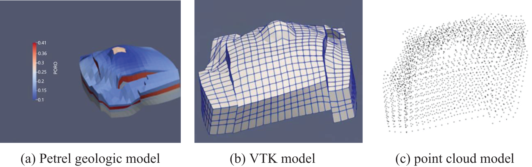
Figure 1: Process of generating point cloud model of reservoir using Adaptive Point Cloud Generation Technology

Convolutional networks, as commonly used intelligent algorithms for point cloud reconstruction, often require regularization of point clouds during reconstruction. Point clouds themselves are irregular, so they must first be regularized before being divided into grids. As a result, this algorithm can lead to a significant number of unnecessary voxel partitions, causing issues such as point cloud sparsity, which seriously affects its stability. Currently, Point Net, as a deep neural network, is widely used for the analysis of point cloud data. The Point Net does not require mapping point clouds into 2D or 3D models. You only need to input the point cloud into the model for processing. The Point Net's network structure is shown in Fig. 2. It primarily consists of a T-Net module, an MLP (Multi-Layer Perceptron) with shared weights, and a max-pooling layer, which respectively addresses the issues of rigid transformation invariance, point correlation in 3D Euclidean space, and the unordered nature of point cloud data. Finally, feature extraction is performed on the entire connected layer, enabling image classification and segmentation.

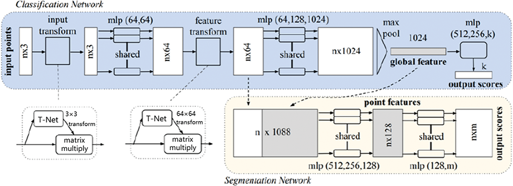
Figure 2: Point Net network structure used in this work

2.1.2 Connectivity Element Method

Provided with the point cloud model, the Connectivity Element Method is then applied to generate the network. The CEM establishes connectivity between grids in a way different from traditional numerical simulations. It replaces the traditional grid topology with unstructured nodes, and simplifies node connectivity units. Based on the node’s influence radius, a series of one-dimensional connectivity units can be constructed. On this basis, flow simulation analysis is performed. The connectivity element system is illustrated in Fig. 3. The principle of CEM is to first select influence domains with an appropriate radius as node centers and establish a one-dimensional connectivity unit system between nodes. Compared to existing discrete fracture models and embedded discrete models, this technique does not require a complex geometric parameter calculation process to obtain the connectivity between grids, which gives it a significant advantage.

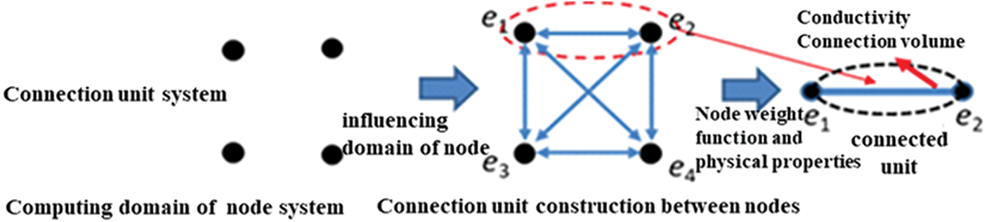
Figure 3: Connection unit system

In order to build the transport equation within the connectivity unit system, it is necessary to compute the characteristic parameters representing the connectivity units. Building upon the principles of INSIM-like methods, this work calculates and solves the characteristic parameters as follows. Firstly, the fluid transport capacity of connectivity units is characterized using the conductivity Ti,j. The connectivity volume Vp,i,j represents the geometric properties of connectivity units. A schematic diagram of the model representation parameters is defined, as shown in Fig. 4, where the blue circles represent well nodes, the red dashed circles represent the connectivity volume within the range centered around well points, and the gray ellipses represent the connectivity volume between wells. Conductivity is the volume flow rate of fluid in the flow channel per unit pressure difference, measured in m3/d/MPa. Connectivity volume represents the capacity of the unit between two nodes to store fluid, measured in cubic meters (m3).

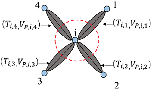
Figure 4: Schematic diagram of model parameter representation

Assuming that the conduction rates between nodes (i,j) computed with node i and node j as the center nodes, respectively:

Tij=αλijkijVi∑m=34em,ji(1)

where k is the permeability in millidarcies (mD), u is the fluid viscosity (water phase, oil phase) in millipascal-seconds (mPa/s), t is time in days, α is the unit conversion factor with a value of 0.0864, V is the control volume of the node, Tij represents the connectivity conductivity between nodes i and j with i as the central node, measured in m3/d/MPa, and Tij represents the connectivity conductivity between nodes i and j with j as the central node, also measured in m3/d/MPa. λij=(kroμo+krwμw)ijtVTijjαAijLijVijiO(m)mG(m)Nu, kro represents the relative permeability of the oil phase, krw represents the relative permeability of the water phase, μo represents the viscosity of the oil phase, and μw represents the viscosity of the water phase.

When using traditional connectivity conductivity, and the sum of the control volumes of all connectivity units equals the total reservoir volume, the calculation expression for the control volume of connectivity units can be obtained as follows:

Vij=GijLij2∑i=1N−1∑i<jNGijLij2⋅VR(2)

where Aij represents the cross-sectional area of adjacent grid sections in square meters (m2), and Lij is the distance between the centers of two grids in meters (m). Vij can be considered as the control volume between grid i and grid j. Gij=αVj∑m=34em,ij. In traditional numerical models, the connectivity volume has a similar relationship with conductivity.

2.2 Parameter Inversion of Connectivity Units in Fractured Reservoirs

2.2.1 Establishment of Historical Matching Objective Function

This project is based on Bayesian theory and focuses on reservoir numerical simulation. It aims to build a dynamic parameter that aligns with mathematical principles, reflects reservoir characteristics, and is closely related to reservoir properties while also being applicable to real-world scenarios. Considering the unique reservoir characteristics of fractured reservoirs, there might be communication between oil and water wells and surrounding aquifers. Therefore, when considering incompressible water bodies, the volume of water is also an important influencing factor that can be adjusted during the fitting process.

Establishing the mathematical model results in the following system of equations:

min O(m)=12[G(m)−dobs]TCd−1[G(m)−dobs],m=[⋯,Tij0,Vij0,⋯]Tmlow≤m≤mupVR,low≤0.5∑i=1Nw∑j=1NwVijk0≤VR,up(3)

where O(m) is the mathematical function for history matching, m is the vector of inversion parameters, which refers to the vector composed of connectivity volume, conductivity, and phase permeability parameters; dobs represents the actual observed values (in conceptual model studies, it refers to the observed values of the true model); G(m) represents the vector composed of production data generated through data-driven models; Cd represents the dynamic covariance matrix. VR is the total effective pore volume of the model in cubic meters (m³); mlow and mup are vectors representing the lower and upper limits of the characteristic parameters, respectively.

2.2.2 History Matching and Inversion Optimization Algorithm

Using the existing method for fitting inter-well connectivity data in fractured reservoirs, a mathematical model for fitting inter-well connectivity data in fractured reservoirs was established. Based on the principle of optimality, it was historically matched and iteratively solved to obtain local minima and their corresponding model parameters. Based on the general formula of the SPSA (Simultaneous Perturbation Stochastic Approximation) gradient method, considering the first-order Taylor expansion and the expected value, we have:

E[g(uoptl)]=E[CU1/2ZlZLTCUT/2∇J(uoptl)]=CU1/2E[ZlZLT]CUT/2∇J(uoptl)(4)

In the equation: uoptl represents the optimal control quantity obtained in the i-th iteration step; εl represents the perturbation step size; Δl represents the random perturbation vector Nu, where the included elements Δli, (i=1,2,…,Nu) follow a symmetric Bernoulli distribution with a parameter of ±1. Under certain conditions, the SPSA gradient based on the covariance matrix of control variables remains an upward gradient, and the expected value is the product of the covariance matrix and the actual gradient.

2.2.3 Establishment of Historical Fitting Constraints

For actual fractured reservoirs composed of vugs, fractures, and matrix, compared to traditional sandstone reservoirs, they exhibit strong heterogeneity. Parameters such as reservoir thickness, permeability, porosity, and pore volume differ significantly. In the inversion process, the initial values of these two parameters (conductivity and connectivity volume) are calculated based on the static reservoir physical properties. Therefore, before conducting model inversion, preliminary geological knowledge should be integrated to impose boundary constraints on these characteristic parameters (conductivity and connectivity volume) to ensure that the inversion results better reflect the real geological features. During history matching, both connection transmissibility and connection volume will be tuned. Restrictions should be set for history matching. In this work, the upper and lower limit of connection transmissibility and connection volume are 0.8 and 1.2, respectively. Note that, though tuned, the summation of connection volume will not be changed.

3  Results and Discussions

3.1 Conceptual Modes for Validation

To validate the accuracy of the connectivity methods for fractured reservoirs presented in this paper, a connectivity model of a fractured reservoir was established using Petrel geological modeling software, as shown in Fig. 5. Then, with the help of Eclipse model for corner-point grid generation, the adaptive point cloud generation technique was used to reconstruct and characterize the reservoir space of fractures and vugs. Independent fractures or vugs were identified and numbered, and characteristic points were extracted for fractures and vugs based on their reservoir features. The CEM method was then employed to discretize and simplify the connectivity units of fractures and vugs. Path tracing simulation was used to calculate the connectivity between fractures and fractures, vugs and fractures, and vugs and vugs, as well as to calculate the connection conductivity and connection volume. Production dynamic predictions were performed using cumulative oil production, water cut, single well oil production rate, water cut, and other dynamic indicators as historical fitting observations. The conductivities and connection volumes of various connectivity units were considered as the characteristic parameters to be modified. Based on the SPSA gradient-free algorithm, the model's characteristic parameters were inverted to make them reflect the actual connectivity of the reservoir more realistically.

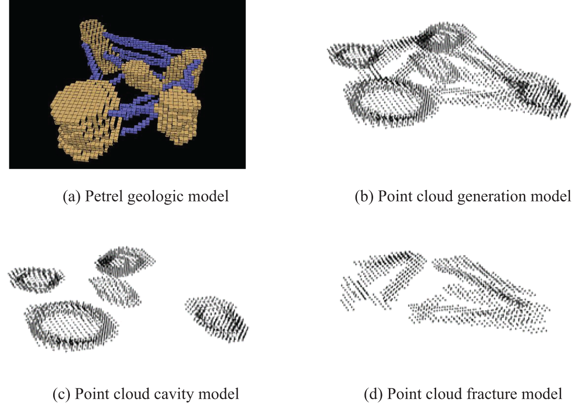
Figure 5: Schematic diagram of processing of conceptual mode

Based on the quantitative recognition and characterization of the three-dimensional connectivity of fractured reservoirs, this work established a conceptual model using Petrel, as shown in Fig. 6a. The model had a grid size of 50 × 50 × 30, with grid dimensions of 5 m × 5 m × 1 m, resulting in 19,447 effective grids. The initial average reservoir pressure was 40 MPa, and the initial water saturation was set to 0.2. The average porosity for vugs and fractures was set at 0.2 and 0.05, respectively, with permeabilities of 4000 mD for vugs and 80 mD for fractures. The model featured five vugs of different sizes and 21 fractures of various scales, forming complex structures. The modeling was carried out using Eclipse software as reference solution, as shown in Fig. 6b. Injection-production development was set up with controlled injection and production rates. The adaptive point cloud generation technique was used to extract characteristic points and construct the CEM connectivity unit system, as shown in Fig. 6c. When characterized using the connectivity unit method, the model has 1398 nodes and 22,769 connection units, and a single simulation (forward modeling) took only 32 s. As comparison, the simulation time using Eclipse takes 2 h.

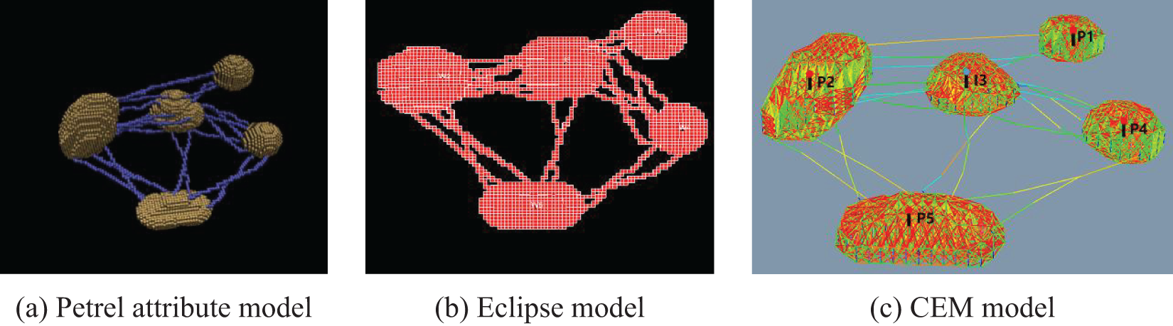
Figure 6: Comparison between the fine grid model and CEM model

A 3-injection-2-production CEM connectivity model was constructed, as shown in Fig. 7. In this model, I2, I3, and I5 represented injection wells with injection rates of 6, 6, and 6 m³/d, respectively. P2 and P4 represented oil production wells with production rates of 8 and 10 m³/d, respectively. The simulation time was 2800 days. Dynamic fitting of single well oil production and water cut was carried out, as illustrated in Fig. 8. In this figure, the blue values represent the results calculated by the Eclipse model, serving as reference solution. The orange values represent the results of forward modeling (or simulation), while the red values represent the results of inverse modeling (or fitting) in this work. Through the adjustment of characteristic parameters, the fitting accuracy can reach over 90%. This validates the accuracy of the proposed model.

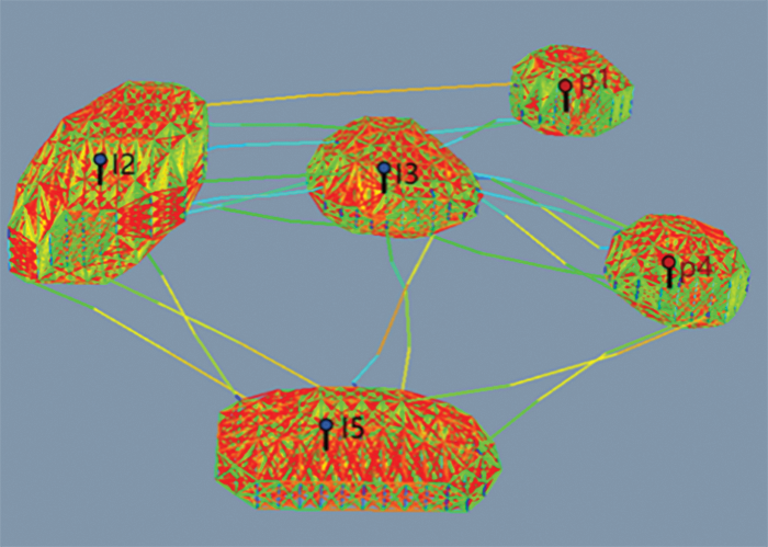
Figure 7: CEM model for 3-injection and 2-production procedure

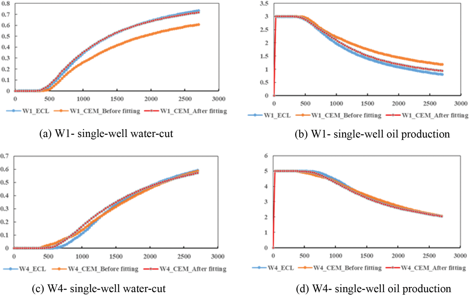
Figure 8: Comparison of simulation results between Eclipse and CEM simulation

Fig. 9 further compares water saturation from Eclipse model and CEM model. Note that the water saturations from CEM are interpolated based on the node saturations. It is observed that there is good match between saturations from the two methods.

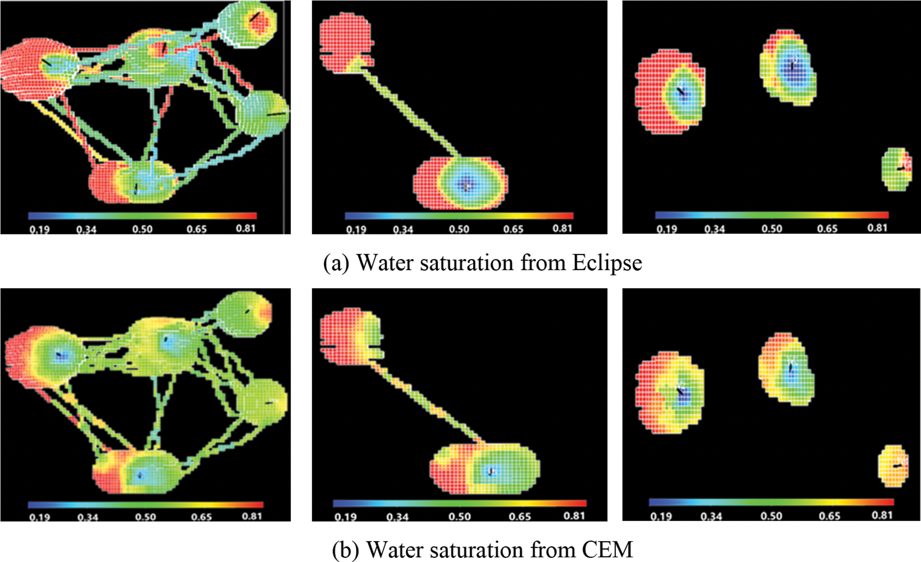
Figure 9: Comparison of water saturation from Eclipse and CEM

3.2 Field Application

We further apply the proposed method to a real fractured-vuggy reservoir in Xinjiang Province, China. In this application, formation is divided into three blocks, consisting of a total of 10 wells. Each well group was used to establish a connection unit model and fit production data, as shown in Fig. 10. When dealing with the actual field block, the first step involved filtering the matrix data of the grid, retaining only the vug-fracture structure. During this process, it was also necessary to filter the parameter data (permeability, porosity, etc.) for each well group in the block. This study will use one of the well groups as an example for illustration.

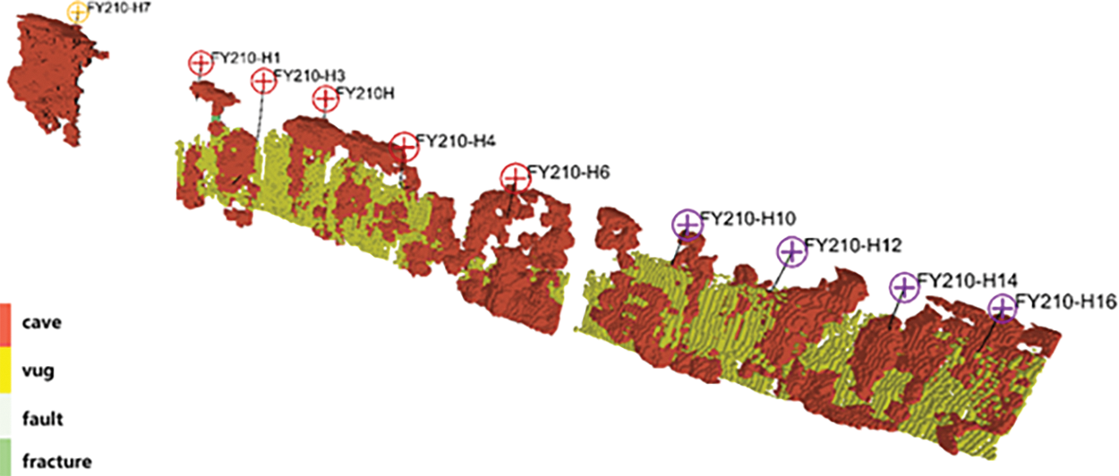
Figure 10: Petrel fine grid model of a fractured-vuggy formation

The central part of the block of this well group, which is a multi-well unit of carbonate reservoirs, has five wells, with a total grid number of 4,494,000 in the block. Fig. 11 shows the comparison between the Petrel model and the CEM model of this well group. In the CEM model, the number of nodes is 1311 and the number of connections is 16,318. The average porosity is 0.032, the initial water saturation is 0.3, the reservoir pore volume is 6.7 × 106 m3, the average initial reservoir pressure is 88 MPa, the rock compression factor is 0.00014, MPa−1, the oil phase compression factor is 0.000426, MPa−1, the water-phase compression coefficient 0.000426 MPa−1, oil-phase viscosity 0.65 mPa/s, oil-phase volume coefficient 1.682, water-phase viscosity 0.233 mPa/s, water-phase volume coefficient 1.0438. Fig. 12 compares the cumulative oil production, water cut, single-well oil production rate with the historical field data. It is shown that by adjusting the characteristic parameters of connection units, the fitting accuracy can reach more than 90%.

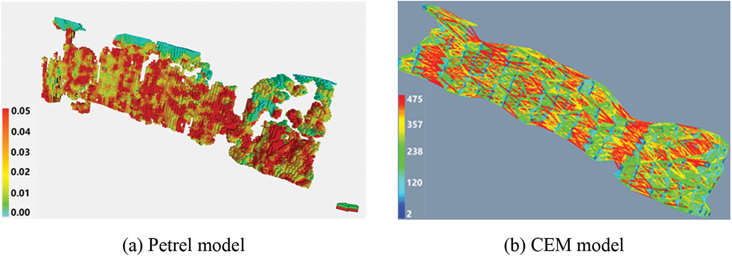
Figure 11: Comparison between the Petrel grid model and the CEM model

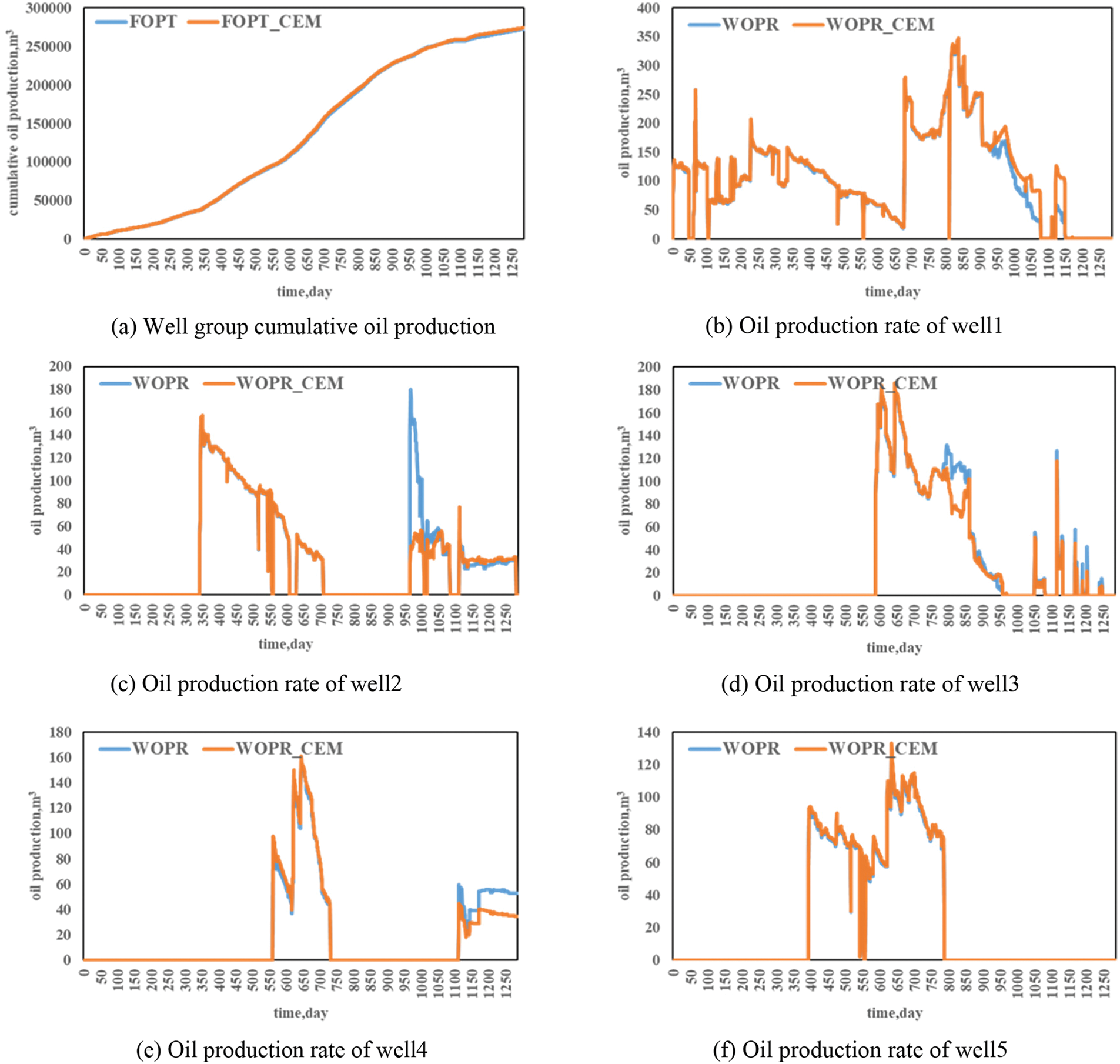
Figure 12: Comparison of simulated results using CEM with history data

4  Conclusions

Based on the adaptive point cloud generation technology, the gridless connective element method can flexibly portray the three-dimensional morphology of fractured-vuggy reservoirs. By establishing the connection unit system, the three-dimensional reservoirs can be efficiently described by two characteristic parameters, namely, the connection conductivity and connection volume. Through the establishment of the conceptual model, it is shown that by the inverse calculation of characteristic parameters and fitting of production data, the established connection model can efficiently and accurately represent the actual fine grid model. The field case study shows the potential of the proposed model in dealing with large-scale problems.

Acknowledgement: None.

Funding Statement: This study is funded by the Natural Science Foundation of Xinjiang Uygur Autonomous Region (No. 2022D01A330), the CNPC (China National Petroleum Corporation) Scientific Research and Technology Development Project (Grant No. 2021DJ1501), National Natural Science Foundation Project (No. 52274030) and “Tianchi Talent” Introduction Plan of Xinjiang Uygur Autonomous Region (2022).

Author Contributions: The authors confirm their contribution to the paper as follows: study conception and design: Xingliang Deng, Peng Cao and Yuhui Zhou; data collection: Yintao Zhang, Xiao Luo, Liang Wang; analysis and interpretation of results: Xingliang Deng, Peng Cao; draft manuscript preparation: Xiao Luo, Liang Wang. All authors reviewed the results and approved the final version of the manuscript.

Availability of Data and Materials: Data supporting this study are included within the article.

Conflicts of Interest: The authors declare that they have no conflicts of interest to report regarding the present study.

References

1. Jin, Z. Y., Cai, L. G. (2007). Inheritance and innovation of marine petroleum geological theory in China. Acta Geologica Sinica, 2007(8), 1017–1024. [Google Scholar]

2. Lu, H. T., Han, J., Zhang, J. B., Liu, Y. L., Li, Y. T. (2021). Development characteristics and formation mechanism of ultra-deep carbonate fault-dissolution body in Shunbei area, Tarim Basin. Petroleum Geology & Experiment, 2021(1), 14–22. [Google Scholar]

3. Qi, L. X., Yun, L. (2020). Carbonate reservoir forming model and exploration in Tarim Basin. Petroleum Geology & Experiment, 2020(5), 867–876. [Google Scholar]

4. Choquette, P. W., Pray, L. C. (1970). Geologic nomenclature and classification of porosity in sedimentary carbonate. AAPG Bulletin, 54(2), 207–250. [Google Scholar]

5. Wang, X. T., Wang, J., Cao, Y. C., Han, J., Wu, K. Y. et al. (2022). Characteristics, formation mechanism and evolution model of Ordovician carbonate fault-controlled reservoirs in the Shunnan area of the Shuntuogole lower uplift, Tarim Basin, China. Marine and Petroleum Geology, 145, 105878. [Google Scholar]

6. Kerans, C. (1988). Karst-controlled reservoir heterogeneity in Ellenberger Group carbonates of west Texas. AAPG Bul1etin, 72(10), 1160–1183. [Google Scholar]

7. Liu, J., Chen, Q. L., Wang, P., You, D. H., Xi, B. B. et al. (2021). Characteristics and main controlling factors of carbonate reservoirs of Middle-Lower Ordovician, Shunnan area, Tarim Basin. Petroleum Geology & Experiment, 2021(1), 23–33. [Google Scholar]

8. Wu, M. L., Chai, X., Zhou, B. H., Li, H., Yan, N. et al. (2022). Connectivity characterization of fractured-vuggy carbonate reservoirs and application. Xinjiang Petroleum Geology, 43(2), 188–193. [Google Scholar]

9. Li, Z. J. (2021). Fault recognition in a fractured-vuggy reservoir. The SEG/AAPG/SEPM First International Meeting for Applied Geoscience & Energy, Denver, USA. [Google Scholar]

10. Tian, F., Luo, X. R., Zhang, W. (2019). Integrated geological-geophysical characterizations of deeply buried fractured-vuggy carbonate reservoirs in Ordovician strata, Tarim Basin. Marine and Petroleum Geology, 99, 292–309. [Google Scholar]

11. Jiang, Y., Zhang, H., Zhang, K., Wang, J., Cui, S. et al. (2022). Reservoir characterization and productivity forecast based on knowledge interaction neural network. Mathematics, 10(9), 1614. [Google Scholar]

12. Li, Y., Hou, J. G., Li, Y. Q. (2016). Features and classified hierarchical modeling of carbonate fracture-cavity reservoirs. Petroleum Exploration and Development, 43(4), 655–662. [Google Scholar]

13. Xiao, Y., Yu, B. S., Guo, H. H. (2020). Fracture prediction method with narrow azimuth seismic data in tazhong district of Tarim Basin. International Journal of Advanced Materials Chemistry and Physics, 3(1), 13–17. [Google Scholar]

14. Guo, H. H., Xiao, Y. (2019). Quantitative engraving technology and application of ordovician carbonate reservoir in Tarim Basin. International Journal of Computational Intelligence Systems and Applications, 7(1), 1–7. [Google Scholar]

15. Zhao, X. Q., Wu, C. D., Ma, B. S., Li, F., Xue, X. H. et al. (2023). Characteristics and Genetic mechanisms of fault-controlled ultra-deep carbonate reservoirs: A case study of ordovician reservoirs in the Tabei Paleo-uplift, Tarim Basin, Western China. Journal of Asian Earth Sciences, 254, 105745. [Google Scholar]

16. Xing, C. Q., Yin, H. J., Li, X. K., Zhao, X. Y., Fu, J. (2018). Well test analysis for fractured and vuggy carbonate reservoirs of well drilling in large scale cave. Energies, 11(1), 80. [Google Scholar]

17. Zhao, H., Kang, Z. J., Zhang, X. S., Sun, H. T., Cao, L. et al. (2016). A physics-based data-driven numerical model for reservoir history matching and prediction with a field application. SPE Journal, 21(6), 2175–2194. https://doi.org/10.2118/173213-PA [Google Scholar] [CrossRef]

18. Zhao, H., Liu, W., Rao, X., Sheng, G. L., Li, H. et al. (2021). INSIM-FPT-3D: A data-driven model for history matching, water-breakthrough prediction and well-connectivity characterization in three-dimensional reservoirs. The SPE Reservoir Simulation Conference. https://doi.org/10.2118/203931-MS [Google Scholar] [CrossRef]

19. Zhao, H., Xu, L. F., Guo, Z. Y., Zhang, Q., Liu, W. et al. (2020). Flow-path tracking strategy in a data-driven interwell numerical simulation model for waterflooding history matching and performance prediction with infill wells. SPE Journal, 25(2), 1007–1025. [Google Scholar]

20. Zhao, H., Kang, Z. J., Sun, H. T., Zhang, S. X., Li, Y. (2016). An interwell connectivity inversion model for waterflooded multilayer reservoirs. Petroleum Exploration and Development, 43, 99–106. [Google Scholar]

21. Zhao, H., Xu, L. F., Guo, Z. Y., Liu, W., Zhang, Q. et al. (2019). A new and fast waterflooding optimization workflow based on INSIM-derived injection efficiency with a field application. Journal of Petroleum Science and Engineering, 179, 1186–1200. [Google Scholar]

22. Liu, W., Zhao, H., Sheng, G. L., Li, A. H., Xu, L. F. et al. (2021). A rapid waterflooding optimization method based on INSIM-FPT data-driven model and its application to threedimensional reservoirs. Fuel, 292, 120219. [Google Scholar]

23. Bello, S. A., Yu, S., Wang, C., Adam, J. M., Li, J. (2020). Deep learning on 3D point clouds. Remote Sensing, 12(11), 1729. [Google Scholar]