A Wind Power Prediction Framework for Distributed Power Grids

1  Introduction

With the promotion of global carbon reduction policies, wind power generation has gained more attention. However, wind power generation is greatly affected by the meteorological environment, and accurate output prediction is required during actual operation [1]. The fluctuation of wind power affects the reliability of wind power grid connection [2], and may also increase system operating costs [3]. As more wind power is connected to the grid in a distributed form, distributed grid stabilization requires higher and higher wind power prediction accuracy.

The inherent variability and uncertainty of wind power can have a significant impact on the grid [4,5], requiring accurate and reliable forecasts of wind power on different time scales [6]. The prediction methods of wind power correspond to the prediction time scale [7], which are mainly classified into three categories according to the prediction time scale: 1) Short-term forecasts within a few hours, mainly considering the stable grid connection of wind power and real-time operation of the grid [8]. 2) Medium-term forecasts spanning a few hours to a week can provide a basis for generation and reserve decisions [9]. 3) Long-term forecasts are at least one week long, or even on a monthly and yearly forecasting scale, and the maintenance and construction of wind farms need to be dependent on this task [10].

Forecasting methods fall into three main categories:

1) Statistical methods are used to perform short-term recursive prediction of wind farm output power based on collected wind turbine power sequences [11]. Statistical methods include differential integrated moving average model (ARIMA) [12], continuous model (PM) [13], Kalman filtering (KF) [14], and principal component analysis (PCA) [15]. Statistical methods require low computational resources, but can only make short-term predictions within a few hours, and the error will significantly increase with the increase of prediction persistence [16].

2) Physical methods first require the implementation of NWP for wind farms, including grid prediction of meteorological factors such as wind speed, humidity, and direction [17], in order to complete wind power prediction for wind farms. The modeling of physical models considers atmospheric motion and geographical environment, and the calculation process reflects the coupling effect of multiple influencing factors. This method maintains stable performance with the extension of the prediction time scale, but relies heavily on computational resources [18], and has high geographic accuracy, which may result in spatiotemporal deviations [19].

3) Artificial Intelligence (AI) methods can be trained with large amounts of historical data to achieve effective fitting for the complex nonlinearities and uncertainties in wind power time series [20]. AI trained with big data has better generalization ability [16], including Gaussian Process (GP) [19], Support Vector Machine (SVM) [21], Evolutionary Algorithms (AI) [22], Neural Networks (NN) [23].

Deep neural networks (DNNs) [24] incorporating big data have demonstrated excellent prediction performance in recent years. Special structures suitable for time series prediction such as Recurrent Neural Networks (RNN) [25], Long Short-Term Memory Networks (LSTM) [26], and hybrid CNN-LSTM models incorporating Convolutional Neural Networks [9,27,28] are widely used for wind power prediction. These network architectures allow deeper mining of time-series evolution features to obtain more accurate wind power forecasts. However, the performance of a single model is still limited.

In order to compensate for the shortcomings of a single method and improve the accuracy of wind power prediction, current research has proposed many combination methods, including combining the prediction results of multiple models [29], using decomposition methods to process input data [30], and adding error correction (EC) models [31]. The combination of four neural network models and one linear model significantly reduces the uncertainty of prediction output [32]. Reference [33] uses variational modal decomposition (VMD) to decompose the input variables into multiple components, and then integrates nine sub models for prediction. After completing the basic prediction, a specialized EC model is trained based on the prediction results [34]. The application of the above prediction strategies has improved prediction accuracy, but the combination of multiple models poses challenges to the combination method and parameter optimization strategy. The increase in input dimensions after variable decomposition and the separate EC model increase the cost of model training.

Based on the discussion and analysis in this article, a wind power prediction framework suitable for distributed power grids is proposed. The main innovations and work are as follows: 1) Combining the weather research and forecast (WRF) model with Kriging interpolation to accurately localize the NWP to the location of a single wind turbine, which improves the geographic accuracy of forecasts in complex terrain. Positioning NWP at each fan position reduces the impact of fan arrangement and terrain. 2) Propose a hybrid deep prediction architecture (TCN-LSTM) combining multiple TCN sub-networks and LSTM to effectively deal with individual turbine output characteristics and complex wake effects between turbines. The proposed model not only combines the advantages of AI and physical methods, but also shares the loss function through end-to-end training, reducing the difficulty of parameter tuning and training costs. 3) Filtering and reconstruction processing of recorded power sequences using VMD to reduce the impact of sequence randomness on accuracy. The reconstructed recorded power sequence removes volatility while not increasing variable dimensions. 4) A wind farm connected to a distributed power grid was used to validate the proposed method, and the results indicate that the proposed method outperforms multiple comparative models in predicting performance.

The paper is structured as follows: Section 2 describes the mathematical modeling and forecasting framework for forecasting. Section 3 details the theory underlying the methodology used in the article. Section 4 is a simulation experiment, which compares the proposed method with multiple comparison models based on three error indicators, and analyzes and discusses the prediction error. Finally, a summary of the entire work is pro-vided in Section 5.

2  Basic Theory and Methodology

2.1 WRF Introduction and Parameter Setting

The WRF model is jointly developed by multiple research institutions such as the NCAR and the NCEP, and is currently widely used as a mesoscale numerical prediction model. The WRF mode has obvious advantages, such as high modularity and layered design, and can be used for parallel computing. The model integrates the most advanced physical process solutions currently available for simulating future atmospheric processes over multiple days.

In this article, the NWP prediction grid for distributed wind farms is provided by the WRF model. Set the grid with three nested layers to 80 × 80 (18 km), 100 × 100 (6 km), 121 × 121 (2 km), including 51 vertical layers, Fig. 1 shows the grid division and simulation range of distributed wind farm. The driving data is provided by the Global Forecasting System (GFS) and is initialized every 6 h.

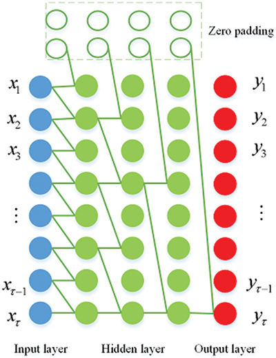
Figure 1: A case study of four layer 1-D convolutional TCN architecture with k = 2, d = 1, 2, 4, 8

2.2 Kriging Interpolation

Kriging interpolation is a commonly used method of interpolating geospatial data to infer values at unknown locations by analyzing spatial correlation of known discrete data points [35]. Its object of study is the regionalized variables in a finite region, and it is a method for linearly optimal and unbiased estimation of spatial data.

Within the designated spatial area, the variable value Z (x) is determined by multiple spatial sampling points xi (i = 1, 2, 3..., n), with each point taking the value Z (xi). Finally, the weighted sum of n known variable values is used to obtain Z*, as shown in Eq. (5).

Z∗=∑i=1nλiZ(xi)(1)

In the equation λi (i = 1, 2, 3..., n) is the weight value of each spatial point, indicating the degree of influence that point has on the current number of points Z* in the region. The solving equation that the weight coefficient needs to satisfy is shown in Eq. (6).

{∑i=1n⁡∑j=1n⁡λiγ(xi,xj)+μ=y(xi,x)∑i=1n⁡λi=1(2)

In Eq. (6), xi represents the spatial position of the i-th sample, and x represents the position of the unknown point. It is necessary to solve for the semi variogram value γ(h) through Formula (7); λi is the weight coefficient; μ is the Lagrange constant. The weight coefficient is obtained from the Kriging equation system, and the estimated value is obtained through Eq. (5).

γ(h)=12E[Z(x)−Z(x+h)]2(3)

2.3 VMD Mathematical Formula

VMD is a signal processing algorithm with adaptive and non recursive modal decomposition characteristics [36]. A typical variational model is as follows:

min{uk}{wk}{∑k‖∂t[(δ(t)+jπt)uk(t)]e−jwkt‖22}(4)

s.t.∑kuk(t)=f(t)

where uk(t) represents the functional expression of the input signal sequence; {uk} denotes the modal set; wk represents the center frequency of the k-th mode corresponding to the initial signal; {wk} represents the center frequency of a decomposed set of modes; f(t) represents the original signal sequence; δ(t) represents the unit pulse function. Eq. (8) introduces Lagrange multipliers λ and quadratic penalty factors α, which can be rewritten as follows:

L({uk},{wk},λ)

α∑k‖∂t[(δ(t)+jπt)uk(t)]e−jwkt||22+||f(t)−∑kuk(t)||22+⟨λ(t),f(t)−∑kuk(t)⟩(5)

Eq. (9) can be solved by the alternating direction method of the multiplication algorithm, and then the modal components of a certain group and the corresponding center frequency can be obtained. The modal can be estimated and solved in the frequency domain according to Eq. (10).

u^kn+1(w)=f^(w)−∑i=1k−1u^in+1(w)−∑i=k+1ku^in(w)+λ^n(w)21+2α(w−wkn)2(6)

where n is the number of iterations; f^(w), u^in+1(w), u^in(w) and λ^n(w) is the form after Fourier transform.

In Eq. (10), the modes in the Fourier domain can be updated. In addition, the modes in the time domain can be obtained by extracting the real part of the inverse Fourier transform of the filtering analysis signal.

wkn+1=∫0∞w|u^in+1(w)|2dw∫0∞|u^in+1(w)|2dw(7)

Finally, the center frequency wkn+1 of the modes needs to be calculated using Eq. (11), and the center frequency will be updated at the center of gravity of the respective modes’ power spectra.

2.4 Temporal Convolutional Network (TCN)

TCN is composed of stacked layers of 1-D CNN, and feature extraction is performed on variable sequences according to time sequence [37]. TCN has two significant characteristics compared to ordinary CNN: 1) when extracting convolutional features, the flow of information strictly follows the order of time before and after; 2) the length of the input sequence is not limited, and the output length remains unchanged after completing the convolution operation.

Fig. 1 shows the computational principle of the TCN network, where the upper level features are obtained through the lower level convolution operation, and the feature sequence has temporal causality. When extracting sequence features, the characteristics of causal convolution make the output of time t determined by time t and previous information during the calculation process, and the feature information flows forward along the time series. The 1-D full CNN structure ensures the consistency of sequence length before and after each layer’s computation. Before each convolution computation, the input sequence is filled with a zero value of k-1, where k is the size of the convolutional kernel of the network in that layer. Eq. (12) provides the calculation process of 1-D causal convolution layer.

F(s)=(x∗f)(s)=∑j=0k−1f(j)x(s−j)(8)

x∈RX represents lower level feature input and f represents a filter: {0,⋯,k−1}→R, F(⋅) represents one layer convolution calculation process.

TCN introduces dilation convolution to solve the gradient training problem caused by too many layers in the network. d represents the dilation factor, and the receptive field of each layer can be calculated as (k-1)d. The calculation principle of each layer’s convolution and network is shown in Eq. (13). In order to ensure that distant historical information can be obtained by the upper layer without causing any omission of lower level information, the general selection of d in the rth hidden layer is 2r−1.

F(s)=(x∗f)(s)=∑j=0k−1f(j)x(s−dj)(9)

In order to solve the gradient optimization problem caused by the excessive number of TCN layers, a residual network was added to skip layers and connect convolutional network layers. The architecture of the residual network is referred to in reference [37]. The residual structure design of TCN is shown in Fig. 2. A residual block consists of two layers of dilated causal convolutions, which are batch-normalized after the convolution operation, using a rectified linear unit (ReLU). Additionally, a dropout is added after each dilated convolution within the residual block used for regularization.

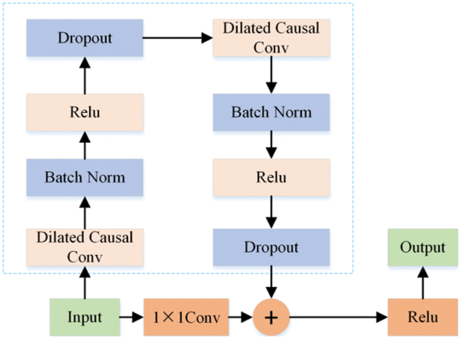
Figure 2: The internal structure of a residual block

2.5 LSTM Mathematical Formula

LSTM has made special improvements to address issues such as RNN gradient vanishing and gradient explosion [38], providing more stable performance in longer-term sequence prediction tasks.

In an LSTM unit (Fig. 3), it consists of three parts: input gate, output gate, and forgetting gate. The calculation process for a single LSTM time unit is as follows:

it=g(wi[xt,st−1]+bi)(10)

ft=g(wf[xt,st−1]+bi)(11)

ot=g(wo[xt,st−1]+bi)(12)

c_int=tanh⁡(wc[xt,st−1]+bc_in)(13)

ct=ftct−1+itc_int(14)

st=ottanh⁡(ct)(15)

where xt indicates lower level input at moment t; st indicates the output of the hidden layer; c_int indicates the output of the previous unit; it indicates the input gate, which decides how much prior information can participate in the calculation of this unit; and ft is the forgetting gate, which controls the level of forgetting in the amount of information in the front layer network; ot represents the output gate, which determines the output information of the current time unit state; where g and tanh serve as the activation function during the training process; and w and b are the weights and deviation values between neurons within each unit.

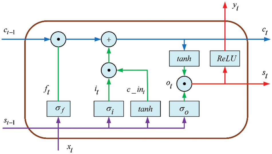
Figure 3: An LSTM time unit architecture

3  Presentation of the Forecasting Framework

3.1 Mathematical Model

The fundamentals of power prediction can be described by a concise formula model:

Z=E(X,Y:ω)X={xt−(n−1)T,xt−(n−2)T,⋯,xt}Y={yt+T,yt+2T,⋯,yt+mT}Z={zt+T,zt+2T,⋯,zt+mT}(16)

X and Y represent the previous wind power series and the wind power series based on the wind speed power conversion curve, respectively. n and m represent the number of time points, T represents the interval between time points, and t represents the current operating time. Z represents the power sequence to be predicted, E(X,Y:ω) represents the mapping calculation between input data and output data, and ω represents the network node parameter set of the prediction model, including network architecture and node weights.

The forecasting model proposed in Eq. (1) enables rolling forecasts for T time intervals in the form of a multi-step sequence of wind power point forecasts for a future period of time. The proposed methodological framework combines NWP-based physical methods with AI deep models.

3.2 Forecasting Process

The prediction process includes multiple stages, and Fig. 4 shows the specific details of the proposed prediction framework. The training and testing data are respectively from the meteorological prediction data output by the WRF model and the historical operating data of each wind turbine provided by the SCADA system.

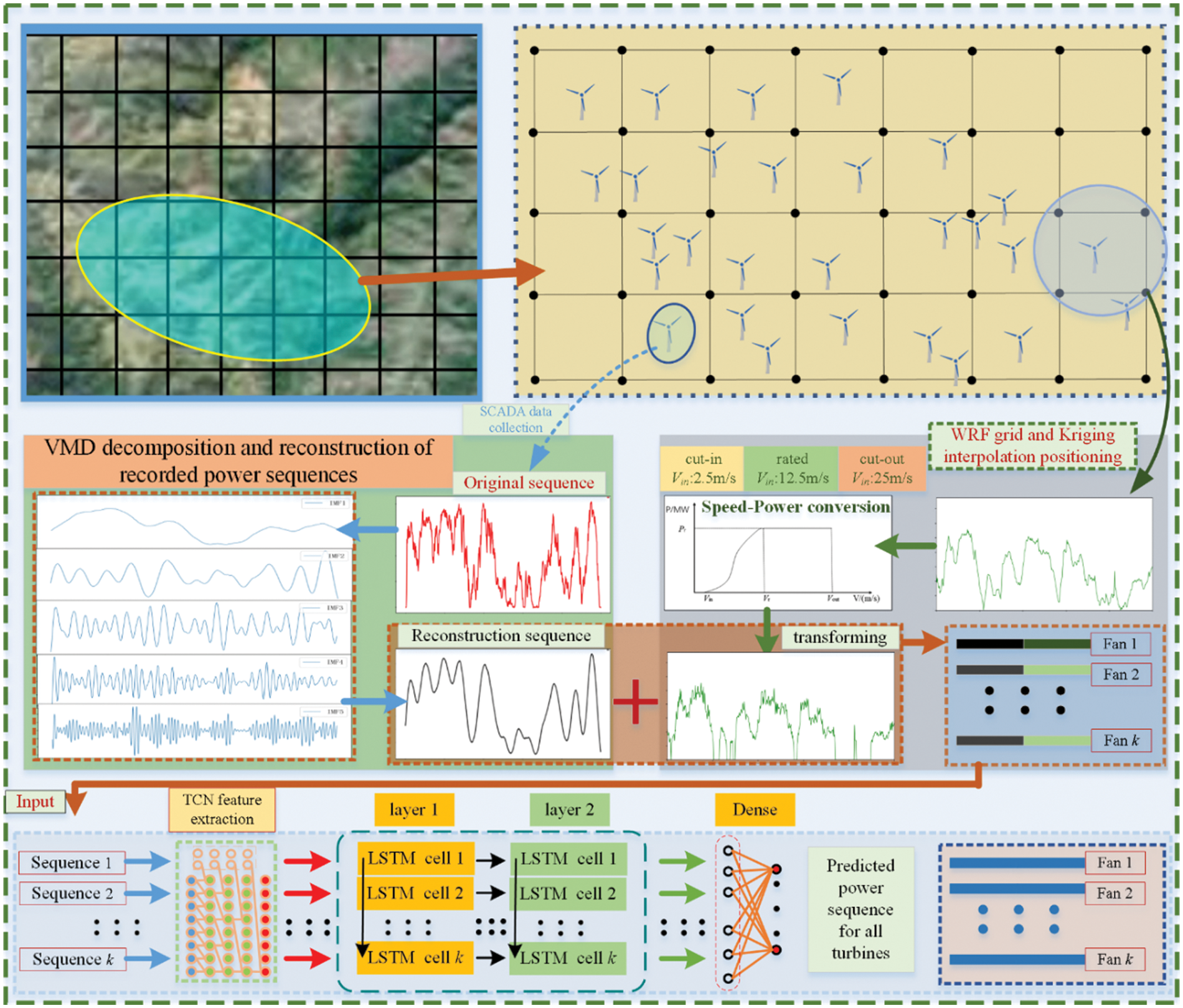
Figure 4: Flow chart of wind power prediction

Firstly, run the WRF mode to extract the innermost geographic grid prediction data based on the geographical location of the wind farm. The case distributed wind farm is from the southeastern part of the mountain, and the turbine distribution terrain is in the mountainous area. The size of the wind turbine distribution area is about 4 × 10 km, and the arrangement of the turbines is extremely irregular due to the mountainous terrain. We used Kriging interpolation to interpolate the four prediction grid wind speed points around the site to the turbine hub height (80 m), and then obtained a preliminary predicted power sequence based on the wind speed-power conversion curves of the turbine manufacturers.

In the daily operation of wind farms, the SCADA system of the wind turbine records equipment operation data, including output power at certain intervals. However, due to the high degree of discreteness in system data collection, historical power exhibits significant volatility and randomness. The obvious random and irregular high-frequency components can affect the predictive performance of the model. After decomposing the recorded power sequence into multiple IMF components by VMD, high-frequency random components can be removed for reconstruction. As shown in the prediction framework in Fig. 1, the volatility of the reconstructed historical power series curve is reduced, which better reflects the actual trend of wind power changes over a period of time. It is important to state that we only process the VMD for the recorded power sequences that are inputs to the model, and the power sequences used to judge the prediction effect are not processed.

After the above processing, the historical power sequence and preliminary predicted power sequence were obtained, we need to perform data sequence splicing. As shown in Fig. 4, after the splicing is completed or obtained the input sequences of all the turbine locations, the number of sequences is k and the length of the sequences is n+m. Where k represents the number of fans, n represents the sequence length of historical wind power, and m represents the sequence length of converted wind power. Each sequence goes into a separate TCN network for timing feature extraction. The input sequence in the TCN network does not change the timing length, and the number of filters determines the feature dimension after completing feature extraction. By adjusting the size of the convolutional kernel to adapt to feature extraction of short sequences. Subsequently the sub-network outputs of the k TCNs are feature merged into a unified LSTM network for feature training. Finally the predicted power sequences of all turbines are output through a fully connected layer.

In the proposed TCN-LSTM model, the input dimensions of the data and the matrix changes during training require careful design. Based on the completed data collection and splicing, the input of each sub TCN network is a one-dimensional time series of n+m. After completing feature extraction through four layers of causal expansion convolution with d = [1, 2, 4, 8,16], the length of the time series remains unchanged, and the number of features increases to 64. At this point, the output of TCN is a two-dimensional array of 64 × (n + m). Subsequently, two LSTM layers were entered for temporal feature learning, with 32 and 64 neurons, respectively. The output of the LSTM layer is still a two-dimensional array of 64 × (n + m), and the feature one-dimensional flattening is performed in the fully connected layer and converted into k predicted wind power sequences with a length of m. Thus, all wind turbines have completed the power prediction task.

3.3 Evaluation Indicators

The performance of model prediction needs to be tested from multiple indicators to evaluate the performance stability of the prediction model. This article uses three indicators, MAE, RMSE, and MAPE, to test the predictive performance of the proposed method and compare the models. The formula is as follows:

MAE=1Q∑j=1Q|p^(j)t+τ−p(j)t+τ|(17)

RMSE=(1Q∑j=1Q(p^(j)t+τ−p(j)t+τ)2)(18)

MAPE=1Q∑j=1K|p^(j)t+τ−p(j)t+τp(j)t+τ|(19)

p^(j)t+τ with p(j)t+τ represent the predicted and true power, t represents the current moment, τ represents the prediction benchmark, and Q represents the number of actual power points used for testing.

4  Case Study

The main work of this section is to evaluate the predictive performance of the proposed method, with a dataset from a wind farm in a distributed power grid, and to compare it with multiple typical methods based on three error indicators. The wind farm that collected data is located in the mountainous area of Southern Shandong, China, and the prediction goal is to predict the multistep power of each wind turbine in the wind farm for the next 6 h. The single wind turbine capacity of the distributed wind farm in the case is 1 MW, with a total of 100 units. The collected data has a time range of 2019 and 2020, including 70176 time points.

4.1 Baseline Methodology

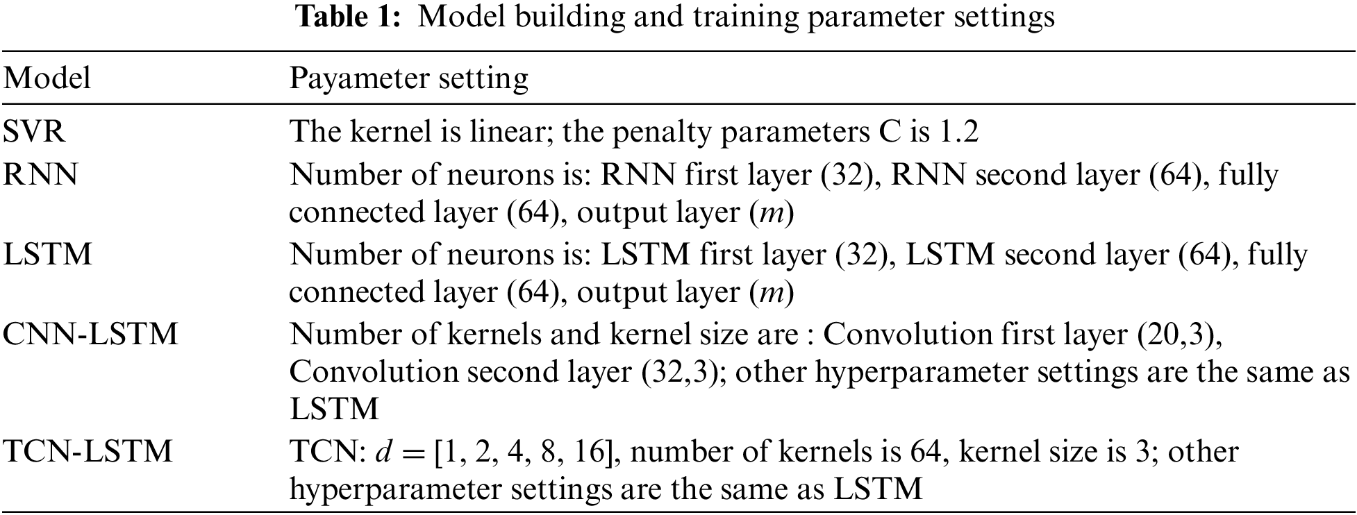
In order to demonstrate the superiority of combining TCN temporal feature ability with LSTM long-term temporal learning ability, the article uses four models: SVR, RNN, LSTM, and CNN-LSTM for wind power prediction, and compares them with the proposed method.

SVR, in fact, is a variant of SVM for regression tasks, which can effectively cope with prediction work. RNN is a special neural network architecture designed for temporal data, which has better learning performance for the evolution trend of temporal data. LSTM is a further improvement of RNN, solving the gradient training problem. The convolutional extraction of the CNN-LSTM hybrid model enhances the feature extraction ability of the data sequence. The parameters of the benchmark algorithm are selected using trial and error methods and determined in conjunction with references.

4.2 TCN-LSTM Model Training

This article uses Python’s Keras modules to build a TCN-LSTM model. The model training process uses the same loss function and optimization algorithm, which is an end-to-end training architecture.

Firstly, the initialization of model parameters is determined by a normal distribution. During the training process, the adaptive moment estimation (Adam) optimization algorithm is used to update the network node parameters [39]. Adam can dynamically adjust the learning rate during the training process, ensuring training speed while avoiding falling into local optima. The training parameters for the other comparative models are presented in Table 1 together.

4.3 Comparison with Baseline Methodology

The dataset is divided according to 4:1 between the training set and the test set. It is first necessary to determine the value of n in Eq. (1), which represents the length of the read history power sequence. When n ≥ 12, the three error indicators tend to stabilize. In order to cope with the complex randomness of the wind power sequence, n = 16 is ultimately determined. The length of the prediction sequence is determined by m in Eq. (1) and can be set according to specific prediction tasks. In actual prediction experiments, this article sets m = 6 to achieve multi-step power prediction for the next 6 h. The test results of MAE, RMSE, and MAPE for the five models are shown in Tables 2 to 4.

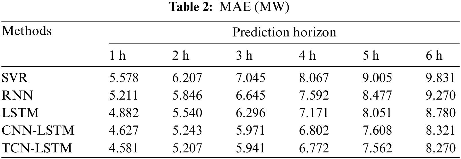
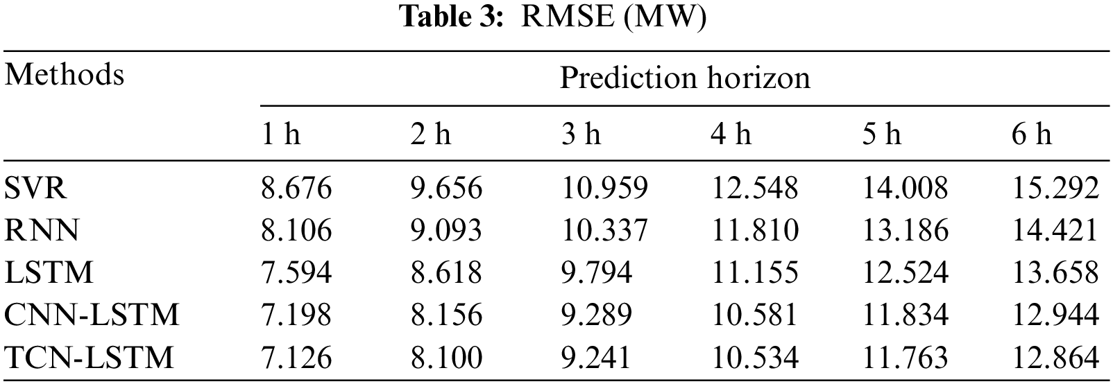
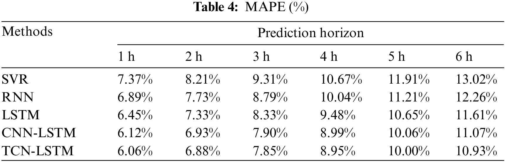
In comparison with the four benchmarks, TCN-LSTM achieved the best prediction results at all prediction levels. Of these, SVR had the worst predictions, which was to be expected. Because the power output of the wind turbine is affected by continuous changes in wind speed, the sequence has obvious temporal characteristics, while the other four prediction models have special designs for time series, which are more suitable for predicting continuously changing wind power sequences. LSTM has better predictive performance than RNN and has been repeatedly validated in other predictive studies [26,40]. This is because the improved working mechanism of LSTM solves the local optimization problem of RNN gradient training, and has better sequence feature learning ability. Adding CNN for feature extraction in front of the LSTM network helps improve the model’s prediction ability, slightly better than simply LSTM in multiple prediction time scales. Overall, it can be concluded that TCN has better feature extraction ability for temporal sequences than ordinary CNN. From the comparison of results, it can be concluded that the proposed method in this paper has obvious superiority in predicting performance.

The performance trends of the four methods are relatively consistent, and the three error indicators significantly decrease with the extension of the prediction horizon. Fig. 5 shows the power comparison of TCN-LSTM with different prediction durations, and the 1 and 2-h prediction curves are very close to the real wind speed curve. Not only is the absolute error basically limited to within 10MW, but trend fitting is also achieved in the peak range of 100–150. As the predicted horizon extends to 4–6 h, the error value gradually increases, and significant outliers will first appear in the range of power series fluctuations. In addition, the trend following effect of the model’s predicted power on real wind power gradually decreases, and the volatility of the sequence curve also decreases.

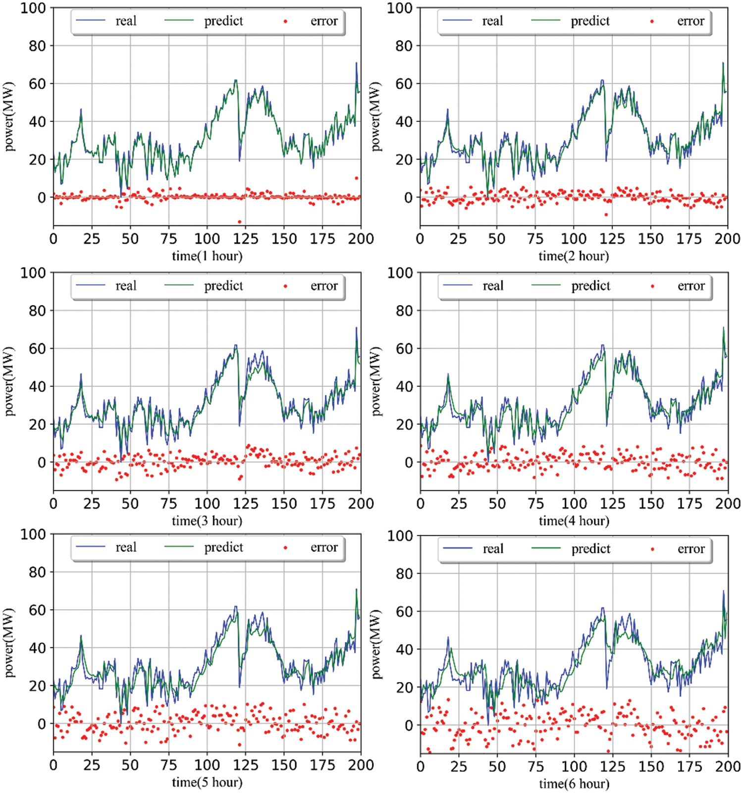
Figure 5: Actual power and predicted power 1–6 h curve and error

4.4 VMD Processing Analysis

The wind power sequence collected by the SCADA system is decomposed into 5 IMFs based on frequency using VMD decomposition (Fig. 4). After gradually removing high-frequency components for reconstruction, the reconstructed sequence is smoother than the original sequence, and some random extreme points are removed.

Fig. 6 shows the trend of test results for MAE, RMSE, and MAPE of the TCN-LSTM model under different IMF component reconstructions. It can be seen that the original sequence IMF (1–5) has the worst prediction performance, and the randomness brought by the recorded power sequence affects the prediction performance of the model. With the gradual removal of high-frequency components, the IMF (1–3) achieved the best prediction performance. However, with the subsequent removal of more components, the error tends to increase. From the perspective of three indicators, the processing of record power de-composition and reconstruction by VMD shows a prediction performance improvement of about 20% compared to the original sequence.

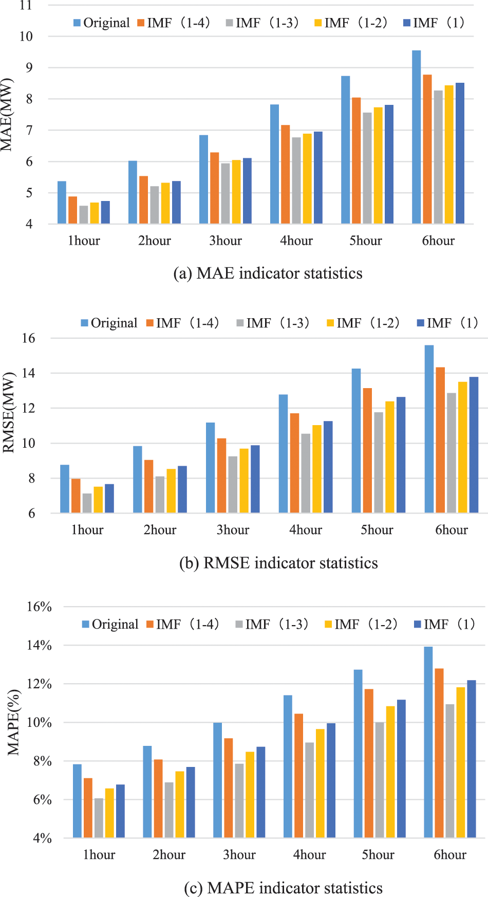
Figure 6: Comparison of prediction effects of different IMF reconstructions in 1–6 h

4.5 Further Error Analysis and Discussion

From the above actual data simulation results, it can be seen that the wind power prediction framework proposed in this article, which is suitable for distributed power grids, has achieved the best prediction results. The method proposed in this article is designed for distributed wind farm power prediction in multiple aspects, and further error analysis and discussion are conducted in this section.

As mentioned throughout the article, the deep model TCN-LSTM of the prediction framework combines artificial intelligence and WRF physical models. The wind power prediction task has obvious spatiotemporal continuity, and the wind speed power conversion curve based solely on wind turbine design will bring significant errors. However, NWP implemented in WRF physical mode may exhibit significant spatiotemporal biases due to the rough initial modeling data, resulting in insufficient accuracy in near prediction. Based on the above two unfavorable factors, the use of the TCN-LSTM depth model combined with a large amount of historical data for secondary prediction improved the accuracy of continuous wind power prediction sequences and to some extent corrected the prediction bias caused by complex terrain. In addition to improving prediction accuracy, the TCN-LSTM depth model also has good universality. By using a single wind turbine equipped with a TCN sub network, all wind turbines in a distributed wind farm are integrated into a unified deep architecture. And an LSTM network is used to receive the out-puts of all TCN subnetworks, taking into account the influence of wind turbine wake in training and prediction, which can simultaneously achieve multi-step power prediction for all wind turbines.

5  Conclusions

This article proposes a wind power prediction framework suitable for distributed power grids. Compared to the benchmark method, the proposed prediction framework exhibits better prediction performance in a distributed wind farm on a mountainous terrain.

Based on the analysis of real case prediction results, the conclusions drawn from this work are summarized as follows:

1) The use of WRF model prediction grid and Kriging interpolation can effectively improve the geographical accuracy of NWP prediction for distributed wind turbines, and to some extent avoid prediction errors caused by mountainous terrain.

2) The TCN-LSTM architecture is very flexible and is not limited by the number and arrangement of wind turbines in the wind farm. It can use an end-to-end trained model to achieve power prediction for all wind turbines at all locations.

3) VMD is used to record power sequence decomposition and reconstruction without adding model input sequences, which can significantly improve prediction performance.

4) TCN-LSTM can also be seen as a secondary prediction of wind power, providing more accurate WSF for wind farm operation.

In future research, we plan to further expand the proposed distributed grid wind power prediction framework, taking into account the actual situation of the wind farm, and introducing meteorological factors such as temperature, pressure, humidity, and wind turbine operation status into the model to further improve the accuracy of wind power prediction.

Acknowledgement: Thanks to all collaborators who have made outstanding contributions to this article, as well as the support of the relevant staff of the Energy Engineering journal.

Funding Statement: This research was funded by National Key Research and Development Program of China (2021YFB2601400).

Author Contributions: Conceptualization, B.C.; Methodology, B.C.; Software, B.C.; Validation, Z.L.; Investigation, B.C., Z.L., S.L., Q.Z.; Writing—original draft, B.C.; Writing—review & editing, L.Z. and X.L.; Funding acquisition, B.C. All authors have read and agreed to the published version of the manuscript.

Availability of Data and Materials: Unfortunately, we hereby declare that the data used in the article comes from the wind farm operator and is accompanied by a confidentiality agreement, and we cannot directly provide the dataset.

Conflicts of Interest: The authors declare that they have no conflicts of interest to report regarding the present study.

References

1. Wang, L., Xue, A. (2023). Wind speed modeling for wind farms based on deterministic broad learning system. Atmosphere, 14, 1308. [Google Scholar]

2. Hu, Q., Su, P., Yu, D., Liu, J. (2014). Pattern-based wind speed prediction based on generalized principal component analysis. IEEE Transactions on Sustainable Energy, 5(3), 866–874. [Google Scholar]

3. Chen, N., Qian, Z., Nabney, I., Meng, X. (2014). Wind power forecasts using gaussian processes and numerical weather prediction. IEEE Transactions on Power Systems, 29, 656–665. [Google Scholar]

4. Khodayar, M., Kaynak, O., Khodayar, M. (2017). Rough deep neural architecture for short-term wind speed forecasting. IEEE Transactions on Industrial Informatics, 13, 2770–2779. [Google Scholar]

5. Rosales-Asensio, E., García-Moya, F., Borge-Diez, D., Colmenar-Santos, A. (2019). Review of wind energy technology and associated market and economic conditions in Spain. Renewable and Sustainable Energy Reviews, 101, 415–427. [Google Scholar]

6. Barbounis, T. G., Theocharis, J. B. (2006). Locally recurrent neural networks for long-term wind speed and power prediction. Neurocomputing, 69, 466–496. [Google Scholar]

7. Simankov, V., Pavel, B., Semen, T., Stefan, O., Anatoliy, K. et al. (2023). Review of estimating and predicting models of the wind energy amount. Energies, 16, 5926. [Google Scholar]

8. Chang, W. (2014). A literature review of wind forecasting methods. Journal of Power Energy English, 2, 161–168. [Google Scholar]

9. Khodayar, M., Wang, J. H. (2019). Spatio-Temporal graph deep neural network for short-term wind speed forecasting. IEEE Transactions on Sustainable Energy, 10, 670–681. [Google Scholar]

10. Chandra, D. R., Kumari, M. S., Sydulu, M., Mussetta, M. (2014). Adaptive wavelet neural network based wind speed forecasting studies. Journal of Electrical Engineering & Technology, 9, 1812–1821. [Google Scholar]

11. Bhaskar, K., Singh, S. N. (2012). AWNN-assisted wind power forecasting using feed-forward neural network. IEEE Transactions on Sustainable Energy, 3, 306–315. [Google Scholar]

12. Chen, P., Pedersen, T., Bak-Jensen, B., Chen, Z. (2010). Arima-based time series model of stochastic wind power generation. IEEE Transactions on Power Systems, 25, 667–676. [Google Scholar]

13. Bludszuweit, H., Dominguez-Navarro, J., Llombart, A. (2008). Statistical analysis of wind power forecast error. IEEE Transactions on Power Systems, 23, 983–991. [Google Scholar]

14. Louka, P., Galanis, G., Siebert, N., Kariniotakis, G., Katsafados, P. et al. (2008). Improvements in wind speed forecasts for wind power prediction purposes using kalman filtering. Journal of Wind Engineering and Industrial Aerodynamics, 96, 2348–2362. [Google Scholar]

15. Hu, Q., Su, P., Yu, D., Liu, J. (2014). Pattern-based wind speed prediction based on generalized principal component analysis. IEEE Transactions on Sustainable Energy, 5, 866–874. [Google Scholar]

16. Zhang, C. Y., Philip Chen, C. L., Gan, M., Chen, L. (2015). Predictive deep boltzmann machine for multiperiod wind speed forecasting. IEEE Transactions on Sustainable Energy, 6, 1416–1425. [Google Scholar]

17. Shirzadi, N., Nasiri, F., Menon, R. P., Monsalvete, P., Kaifel, A. et al. (2023). Smart urban wind power forecasting: Integrating weibull distribution, recurrent neural networks, and numerical weather prediction. Energies, 16, 6208. [Google Scholar]

18. Andrade, J. R., Bessa, R. J. (2017). Improving renewable energy forecasting with a grid of numerical weather predictions. IEEE Transactions on Sustainable Energy, 4, 1571–1580. [Google Scholar]

19. Chen, N., Qian, Z., Nabney, I. T., Meng, X. (2014). Wind power forecasts using Gaussian processes and numerical weather prediction. IEEE Transactions on Power Systems, 29, 656–665. [Google Scholar]

20. Xu, Q. Y., He, D. W., Zhang, N., Kang, C., Xia, Q. et al. (2015). A short-term wind power forecasting approach with adjustment of numerical weather prediction input by data mining. IEEE Transactions on Sustainable Energy, 6, 1283–1291. [Google Scholar]

21. Zeng, J., Qiao, W. (2012). Short-term wind power prediction using a wavelet support vector machine. IEEE Transactions on Sustainable Energy, 3, 255–264. [Google Scholar]

22. El-attar, E. E. (2011). Short term wind power prediction using evolutionary optimized local support vector regression. 2011 2nd IEEE PES International Conference and Exhibition on Innovative Smart Grid Technologies (ISGT Europe), pp. 1–7. [Google Scholar]

23. Quan, H., Srinivasan, D., Khosravi, A. (2014). Short-term load and wind power forecasting using neural network-based prediction intervals. IEEE Transactions on Neural Networks and Learning Systems, 25, 303–315. [Google Scholar] [PubMed]

24. Marino, D. L., Amarasinghe, K. M., Manic, M. (2016). Building energy load forecasting using deep neural networks. Proceedings of the IECON 42nd Annual Conference of the IEEE Industrial Electronics Society, pp. 7046–7051. Florence, Italy. [Google Scholar]

25. Barbounis, T. G., Theocharis, J. B. (2005). Locally recurrent neural networks optimal filtering algorithms: Application to wind speed prediction using spatial correlation. 2005 IEEE International Joint Conference on Neural Networks, pp. 2711–2716. Canada. [Google Scholar]

26. Liu, B. T., Xie, Y. Q., Wang, K., Yu, L. Z., Zhou, Y. et al. (2023). Short-term multi-step wind direction prediction based on OVMD quadratic decomposition and LSTM. Sustainability, 15, 11746. [Google Scholar]

27. Woo, S., Park, J., Park, J., Manuel, L. (2020). Wind field-based short-term turbine response forecasting by stacked dilated convo-lutional LSTMs. IEEE Transactions on Sustainable Energy, 11, 2294–2304. [Google Scholar]

28. Subin, I., Xie, H., Hur, D., Yoon, M. (2023). Comparison and enhancement of machine learning algorithms for wind t urbine output prediction with insufficient data. Energies, 16, 5810. [Google Scholar]

29. Khosravi, A., Machado, L., Nunes, R. O. (2018). Time-series prediction of wind speed using machine learning algorithms: A case study Osorio wind farm, Brazil. Applied Energy, 224, 550–566. [Google Scholar]

30. Wang, J. H., Niu, T., Lu, H. Y., Guo, Z. H., Yang, W. D. et al. (2018). An analysis-forecast system for uncertainty modeling of wind speed: A case study of large-scale wind farms. Applied Energy, 211, 492–512. [Google Scholar]

31. Liu, H., Chen, C. (2019). Multi-objective data-ensemble wind speed forecasting model with stacked sparse autoencoder and adaptive decomposition-based error correction. Applied Energy, 254, 113686. [Google Scholar]

32. Niu, X. S., Wang, J. Y. (2019). A combined model based on data preprocessing strategy and multi-objective optimization algorithm for short-term wind speed forecasting. Applied Energy, 241, 519–539. [Google Scholar]

33. Zhang, L. F., Wang, J. Z., Niu, X. S., Liu, Z. K. (2021). Ensemble wind speed forecasting with multi-objective Archimedes optimization algorithm and sub-model selection. Applied Energy, 301, 117449. [Google Scholar]

34. Li, C. S., Tang, G., Xue, X. M., Saeed, A., Hu, X. (2020). Short-term wind speed interval prediction based on ensemble GRU model. IEEE Transactions on Sustainable Energy, 11(3), 1370–1380. [Google Scholar]

35. Matheron, G. (1963). Principles of geostatistics. Economic Geology, 58(8), 1246–1266. [Google Scholar]

36. Dragomiretskiy, K., Zosso, D. (2014). Variational mode decomposition. IEEE Transactions on Signal Processing, 62, 531–544. [Google Scholar]

37. Bai, S. J., Kolter, J. Z., Koltun, V. (2018). An empirical evaluation of generic convolutional and recurrent networks for sequence modeling. arXiv preprint arXiv:1803.01271. [Google Scholar]

38. Hochreiter, S., Schmidhuber, J. (1997). Long short-term memory. Neural Computation, 9, 1735–1780. [Google Scholar] [PubMed]

39. Kingma, D. P., Ba, J. L. (2015). Adam: A method for stochastic optimization. Computer Science. https://doi.org/10.48550/arXiv.1412.6980 [Google Scholar] [CrossRef]

40. Strobelt, H., Gehrmann, S., Pfister, H., Rush, A. M. (2018). LSTMVis: A tool for visual analysis of hidden state dynamics in recurrent neural networks. IEEE Transactions on Visualization and Computer Graphics, 24, 667–676. [Google Scholar] [PubMed]