Research on Scheduling Strategy of Flexible Interconnection Distribution Network Considering Distributed Photovoltaic and Hydrogen Energy Storage

Nomenclature

1  Introduction

To reduce environmental pollution and achieve the dual-carbon goal, China is vigorously promoting the development of renewable energy. Distributed PV has attracted a lot of attention due to its advantages such as flexible installation, low construction cost, and low fault impact. Although PV has great potential, its random fluctuation is strong, and the grid connection of a high proportion of distributed PV will lead to a substantial increase in power generation fluctuation, which may cause problems such as system line overload, power imbalance, and voltage over the limit, which will affect the operation of the distribution network [1–3].

Given the above problems, although the gas turbine fast response unit can be used to suppress the system fluctuations caused by distributed PV, the gas turbine needs to burn fossil fuels, which reduces the economic and environmental benefits brought by PV power generation, and the appropriate energy storage device can store excess electric energy and promote the timely consumption of PV power, which is a more economic and environmental protection means [4,5]. Reference [6] proposed a joint planning model of distributed power supply and energy storage for active distribution networks by using a two-layer programming method. An improved binary particle swarm optimization (IBPSO) algorithm based on chaos optimization is proposed, which realizes the optimal joint planning by alternating iterations between the two layers. Reference [7] combined distributed generator (DG) and battery energy storage system (BESS), and used a multi-objective evolutionary algorithm based on decomposition (MOEA/D) to s reduce the energy not supplied (ENS) of 30-bus and 69-bus distribution networks. Based on the combined operation of wind and coal, Reference [8] proposed a combined wind and coal energy storage system by adding a lithium iron and phosphorus battery energy storage system (LIPBESS) to adjust the system load. Reference [9] proposed an improved energy management strategy based on the combination of real-time electricity price and electricity state and used this strategy to optimize the allocation of energy storage capacity. In references [6–9], considering the regulating role of energy storage systems in distribution networks, battery energy storage with fast response is selected for adjustment. However, its storage time is short, which is generally only used for intra-day adjustment, and it is difficult to realize seasonal energy scheduling.

To achieve medium-long time-scale scheduling, seasonal energy storage, which supports long-term, large-scale, and wide-area spatial energy transfer, has become a key technology to cope with the high proportion of renewable energy access in the distribution network. Compared with seasonal energy storage methods such as pumped storage and compressed air energy storage, HS is convenient for expansion, less affected by geographical location, multiple storage methods, and energy conversion forms, and can achieve cross-regional transportation, with better storage effect [10,11]. At present, there have been some studies on SHS. Reference [12], aiming at the minimum annual total cost of hydrogen, established a dual-layer mixed integer programming model for an integrated electric-hydrogen energy system. By adjusting the proportion of renewable energy equipment in the system and purchasing power from the upper power grid, the price of hydrogen supply in the planning stage can be effectively reduced. Reference [13] established a two-stage stochastic programming model for hydrogen production, HS, and CCGT system, and proposed the minimum mean difference-entropy weight method to select typical years and the seasonal decomposition method of time series to establish the typical scenario set of stochastic planning. Reference [14] proposed an electric hydrogen integrated energy system (EH-IES) planning model considering hydrogen production and hydrogen storage technologies, which adopts a method combining robust optimization and stochastic optimization to deal with generation load uncertainty and N-1 contingency. References [12–14] have studied HS from the aspects of electric-hydrogen integration, the combination of HS with CCGT, and the planning of a comprehensive electric-hydrogen energy system, focusing on the analysis of the principle of SHS. However, because of the fluctuation characteristics of renewable energy under different time scales, the combination of SHS and short-term energy storage has rarely been involved. On this basis, this paper puts forward a hybrid energy storage system combining SHS and battery energy storage and points out its specific operation flow.

In addition to adding energy storage equipment, we can also start from the perspective of improving the distribution network to improve the economy and power quality of the grid. The use of flexible interconnection technology to build the AC/DC hybrid distribution network can eliminate the AC/DC commutation link and only control voltage, and the controllability and reliability of the system based on power electronics technology will be further improved [15]. In a flexible interconnected distribution network (FIDN) based on soft open point (SOP), Reference [16] proposed a two-stage optimization strategy based on location selection, capacity determination, and optimal operation of key distribution network equipment, considering the loss characteristics of distribution transformers and key distribution network equipment. Reference [17] proposed a flexible economic scheduling method for AC/DC distribution networks considering wind power uncertainty and used non-parametric kernel density estimation and confidence interval method to realize constraint transformation. Reference [18] proposed a two-stage optimization method based on interval optimization to adjust voltage fluctuations and improve the economy of the distribution network with soft open points of energy storage and a high penetration rate of distributed power supply. Reference [19] combined flexible interconnection technology with energy storage devices, studied and proposed a power optimization cooperative control strategy of flexible fast interconnection device with energy storage, to realize power complementarity between feeders. References [16,17] did not consider the role of energy storage in system regulation and only used flexible interconnection technology for regulation. References [18,19] adopted flexible interconnection devices including energy storage for regulation. Although the role of energy storage was taken into account, the scale of energy storage could only be adjusted in a short period, and the differences between different seasons could not be optimized for scheduling. Therefore, the combination of long-term energy storage and flexible interconnection technology to achieve real-time energy supply and demand balance and adjust the seasonal fluctuations of renewable energy is a worthy research direction.

Based on the above, this paper proposes a flexible interconnection distribution network system scheduling strategy that considers distributed PV and HS, that is, HS and flexible interconnection technology are used to promote PV consumption and reduce the impact of the high proportion of distributed PV access on the distribution network. The research work carried out in this paper is as follows:

(1) Based on AC/DC hybrid distribution network considering flexible interconnection, a SHS model is proposed, and a coordinated scheduling strategy model of HS and distributed PV is established.

(2) A multi-objective optimization model with minimum total active power loss, minimum node voltage deviation, and minimum operating cost as objective functions is proposed, and the NSGA-II algorithm is used to calculate the optimization objectives.

(3) Simulation verification is carried out on the improved IEEE33-node distribution network system, the operation results of related equipment of the energy storage system are analyzed, and multiple scenarios are set according to whether HS and flexible interconnection technology are considered. The simulation results show that the optimized scheduling strategy proposed in this paper can effectively improve the economy of the distribution network and improve the power quality of the system.

The rest of this article is structured as follows. The second section introduces the models of distributed PV and HS. The third section introduces the scheduling optimization model of a flexible interconnected distribution network. The fourth section carries on the simulation analysis. The fifth section summarizes the full article.

2  Distributed PV and HS Models

2.1 System Energy Flow Analysis

The distribution network investigated in this study is characterized by a substantial presence of PV and HS components, and the energy flow within the system is illustrated in Fig. 1. The system is primarily divided into three main components: the supply side, the conversion side, and the load side. On the supply side, we have the power grid and PV arrays, which are responsible for electricity generation. The conversion side involves the conversion of electrical energy and comprises a HS system consisting of the electrolyzer (EL), the hydrogen storage tank (HST), and the hydrogen fuel cell (HFC). This system is tasked with transforming surplus electrical energy into hydrogen through the EL. Subsequently, when the power grid experiences shortages, the HFC converts hydrogen back into electric energy, which is then fed back into the grid, facilitating the timely absorption of PV-generated power. The load side primarily comprises electrical loads, serving as the component that consumes the electric energy.

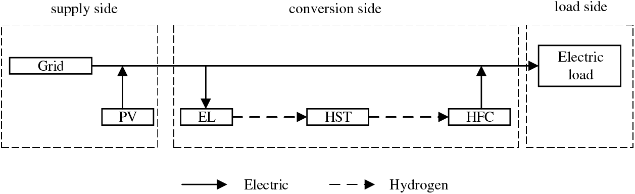
Figure 1: Energy flow diagram of distribution network system

2.2 Distributed PV Model

Since the PV output depends on the light intensity, there is uncertainty. Existing studies have shown that solar irradiance approximately follows Beta distribution [20] in a certain period, and its probability density function is shown in Eq. (1):

f(r)=Γ(π+ω)Γ(π)Γ(ω)(rrmax)π−1(1−rrmax)ω−1(1)

where r and rmax are the actual light intensity and maximum light intensity in a certain period (unit is W/m2), respectively; Γ is the Gamma function; π and ω are Beta distributed shape parameters.

The output power expression of PV [21] can be expressed as follows:

PPV(t)=PSTCGC(t)GSTC{1+kp[TC(t)−TSTC]}(2)

TC(t)=Ta(t)+GC(t)800×(TSTC−20)(3)

where PPV(t) represents the actual output power of photovoltaic cell during period t; PSTC represents the maximum output power of photovoltaic cell under standard test conditions (solar irradiation intensity GSTC is 1000 W/m2, battery surface temperature TSTC is 25°C); GC(t) indicates the actual light intensity of the photovoltaic cell during period t; kp is 0.00485/°C, which is the power temperature coefficient; TC(t) indicates the actual surface temperature of the photovoltaic cell during period t, which can be estimated by the specific ambient temperature and light intensity; Ta(t) indicates the ambient temperature.

In this paper, the Monte Carlo method and the K-means clustering method are used respectively to achieve scene generation and scene reduction [4]. By analyzing and calculating a large number of historical data, a deterministic typical scene is generated to reduce the processing difficulty of complex historical data.

2.3 HS Model

2.3.1 Conventional HS Model

The operational mechanism of the HS utilization link is illustrated in Fig. 2. The EL, HST, and HFC collectively constitute the HS system, forming an efficient electric-hydrogen-electric energy circulation loop. When the PV output exceeds immediate consumption requirements, the surplus electricity is directed into the EL, where it undergoes electrolysis to produce hydrogen, subsequently stored in the HST. Conversely, during periods of power grid demand exceeding supply, hydrogen stored in the HST is directed to the HFC. Through chemical reactions, this hydrogen is converted back into electric energy, which is then fed into the power grid to meet load requirements.

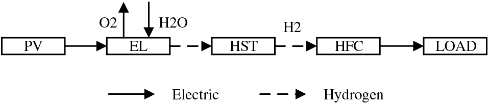
Figure 2: Operation mechanism of HS utilization link

(1) EL

Currently, water electrolysis stands as a prevalent method for hydrogen production, with the EL playing a pivotal role in this process. The EL is instrumental in ionizing water into hydrogen and oxygen, facilitating the conversion of electrical energy into hydrogen energy [13]. The mathematical model for the EL can be represented as follows:

PEL,t=ηELPEL,tin(4)

PEL,min≤PEL,tin≤PEL,max(5)

ΔPEL,min≤PEL,t+1in−PEL,tin≤ΔPEL,max(6)

where PEL,tin and PEL,tout are the input and output power of the EL during the period t, respectively; ηEL is the conversion efficiency of the EL; PEL,max and PEL,min are the upper and lower limits of the input power of the EL, respectively; ΔPEL,max and ΔPEL,min are the upper and lower climbing limits of the EL, respectively.

(2) HST

The HST serves the purpose of storing hydrogen generated by the EL and facilitating its transfer to the HFC. During periods of surplus power within the system, the EL initiates electric-hydrogen conversion, increasing the hydrogen content of the HST. Conversely, during power deficits in the system, the HFC becomes active for hydrogen-electricity conversion, leading to a reduction in hydrogen stored in the HST. In this paper, we focus on the energy transmission process and simplify the intricate compression and hydrogen conversion processes occurring within the HST [22]. Therefore, the mathematical model for the HST can be expressed as follows:

Et+1=Et+ηinPt+1in−Pt+1outηout(7)

Emin≤Et≤Emax(8)

Pminin≤Ptin≤Pmaxin(9)

Pminout≤Ptout≤Pmaxout(10)

PtinPtout=0(11)

ET=E1(12)

where Et is the storage capacity of HST during the period t; Ptin and Ptout are the input and output power of the HST during the period t, respectively; Emax and Emin are the upper and lower limits of HST capacity, respectively; Pmaxin, Pminin and Pmaxout, Pminout are the upper and lower limits of the input and output power of the HST, respectively; ηin and ηout are hydrogen storage and hydrogen discharge efficiency of HST, respectively.

(3) HFC

The HFC is the device responsible for the conversion of hydrogen into electrical energy. When integrated with the EL, the HFC facilitates a two-stage conversion process, converting electrical energy into hydrogen and then back into electricity. This dual conversion process effectively accomplishes the absorption and compensation of electrical energy fluctuations generated by distributed PV [23]. The mathematical model for the HFC can be expressed as follows:

PHFC,t=ηHFCPHFC,tin(13)

PHFC,min≤PHFC,tin≤PHFC,max(14)

ΔPHFC,min≤PHFC,t+1in−PHFC,tin≤ΔPHFC,max(15)

where PHFC,tin and PHFC,tout are the input and output power of the HFC during the period t, respectively; ηHFC is the conversion efficiency of HFC; PHFC,min and PHFC,max are the upper and lower limits of input power of HFC, respectively; ΔPHFC,min and ΔPHFC,max are the upper and lower climbing limits of HFC, respectively.

2.3.2 SHS Model

In Fig. 3, we observe the storage capacity and duration of various energy storage methods. The figure illustrates that conventional energy storage typically focuses on short-term adjustments within a day, often with an adjustment window of less than one week, with the majority of adjustments occurring within 24 h. In contrast, HS demonstrates a remarkable capacity for adjustments ranging from hourly to seasonal, offering a broader range of adaptability and more robust adjustment capabilities.

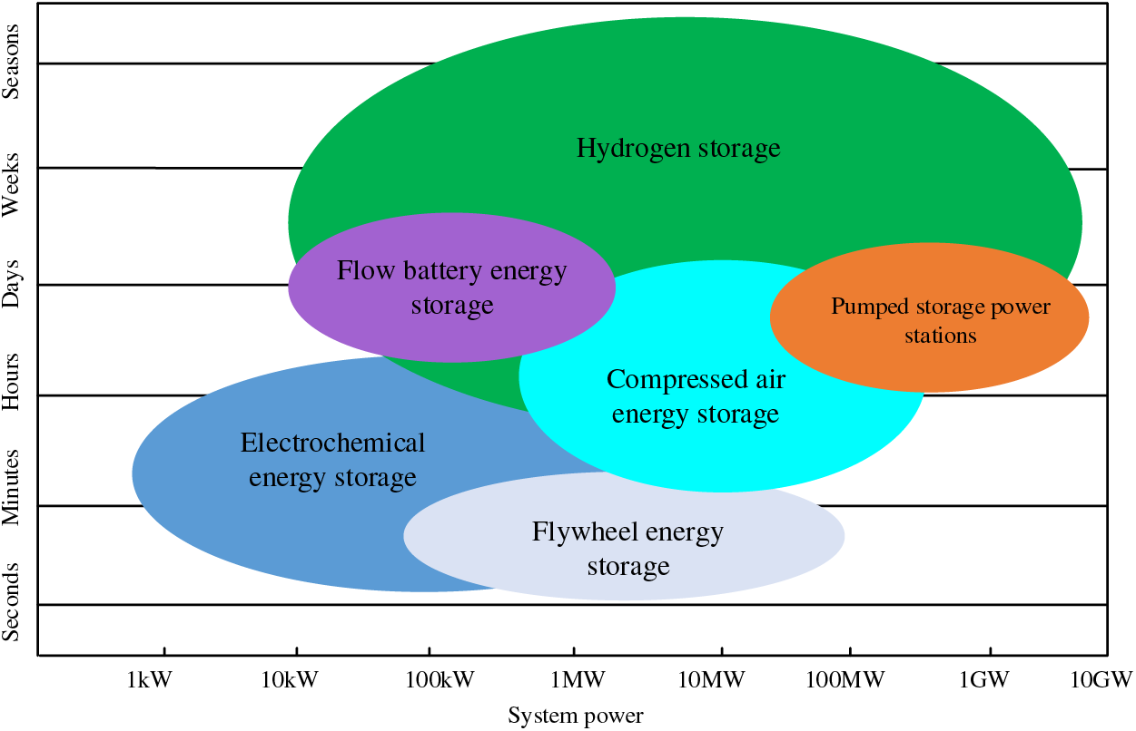
Figure 3: Storage power and time of different energy storage methods

(1) SHS

Compared with conventional HS, SHS involves a longer adjustment time. To streamline calculations, a minimum adjustment period of one day is employed for SHS, allowing it to have a single charge or discharge within 24 h. In the initial scenario, the SHS begins with an initial value equal to half of its installed capacity. On subsequent typical days, the initial value of SHS is derived by summing the charge and discharge power accumulated during the previous season, adjusted for self-discharge energy losses [12].

{λSHS,s,tinPSHS,minin≤PSHS,s,tin≤λSHS,s,tinPSHS,maxinλSHS,s,toutPSHS,minout≤PSHS,s,tout≤λSHS,s,toutPSHS,maxout0.2CapSHS,min≤PSHS,s,t≤0.8CapSHS,max;∀s,t(16)

{ESHS,1,0=0.5CapSHSESHS,1,t=(1−γSHS,loss)ESHS,1,t−1+(ηSHSin⋅PSHS,1,tin−PSHS,1,tout/ηSHSout)Δt;∀t(17)

{ESHS,s,0=(1−365γSHS,lossω(s−1)△t)(ESHS,s−1,0+365⋅ω(s−1)(ESHS,s−1,24−ESHS,s−1,0));∀2≤s≤Ns,tESHS,s,t=(1−γSHS,loss)ESHS,s,t−1+(PSHS,s,tin⋅ηSHSin−PSHS,s,tout/ηSHSout)△t(18)

ESHS,1,0=ESHS,Ns,24(19)

λSHS,s,tin+λSHS,s,tout≤1;∀s,t(20)

{λSHS,s,tin≤λsin≤∑t=1NtλSHS,s,tinλSHS,s,tout≤λsout≤∑t=1NtλSHS,s,toutλsin+λsout≤1;∀s,t(21)

where PSHS,s,t, PSHS,s,tin and PSHS,s,tout are the power, charging power, and discharging power of SHS in the scenario s during the period t, respectively; PSHS,minin and PSHS,maxin are the upper and lower limits of charging power of SHS in scenario s during the period t, respectively; PSHS,minout and PSHS,maxout are the upper and lower limits of the discharge power of SHS in scenario 4 during the period t, respectively; λSHS,s,tin and λSHS,s,tout are the charging and discharging states of SHS in scenario s during the period t, with a state of 1 if present and 0 if not present; CapSHS indicates the capacity of SHS; ESHS,s,t is the energy storage of SHS in scenario s during the period t; γSHS,loss is the self-loss rate of SHS; ηSHSin and ηSHSout are the charging and discharging efficiency of SHS; ω(s) is the probability of scenario s.

(2) Integrated Energy Storage System Considering SHS

Renewable energy and load exhibit distinct fluctuation patterns across various time scales. As a result, a high-proportion renewable energy power system imposes varying requirements on energy storage devices to address these fluctuations. Building upon conventional HS, a comprehensive energy storage system is formed by combining HS with BT energy storage. This combined system facilitates adjustments spanning from a few minutes to several months. Within this framework, short-term energy storage serves the purpose of managing intraday peak loads and maintaining system frequency, ensuring a real-time balance between energy supply and demand. Seasonal energy storage, on the other hand, plays a critical role in mitigating seasonal fluctuations in renewable energy, promoting seasonal demand side response, and fostering increased consumption of renewable energy [12]. The structural configuration of this system is presented in Fig. 4.

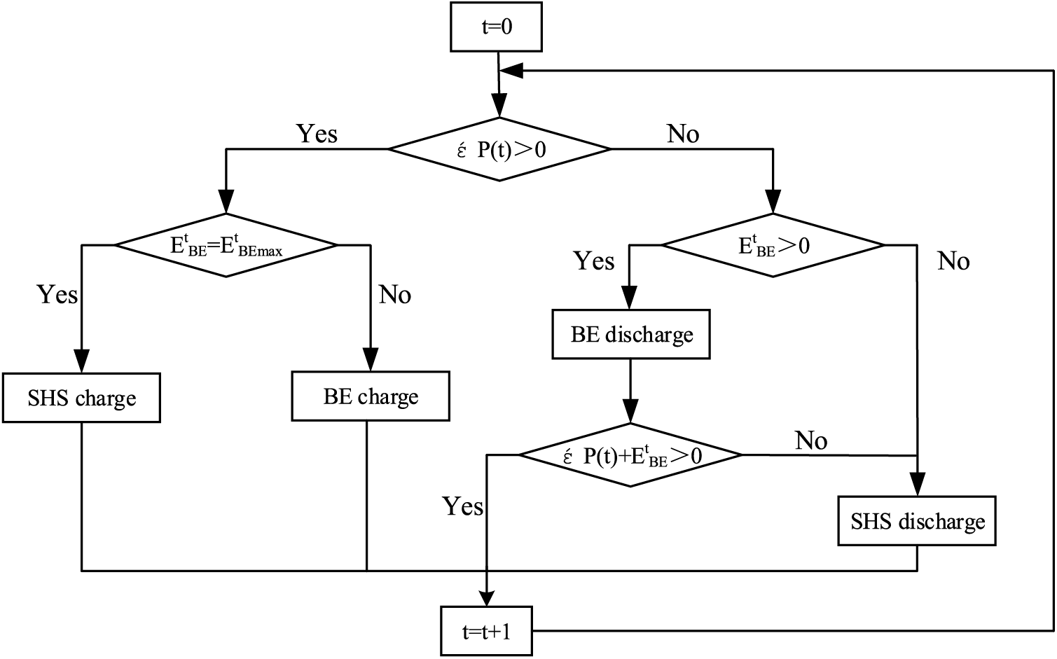
Figure 4: Integrated energy storage system with SHS

In this energy storage system, the response speed of BT energy storage is fast, and the BT is preferentially used for charging and discharging, followed by SHS. Set the net load ΔP(t)=PPV(t)−PLoss(t), when ΔP(t)>0, there is excess energy in the system, the energy storage system can be charged, if the BT is not full, the BT is charged first, when the BT is full, the SHS is charged. If ΔP(t)≤0, the distributed PV output in the system cannot support the load demand, the energy storage system is called and the BT is discharged preferentially. If the BT can support the net load, the cycle is carried out in the next period, otherwise, the SHS is called for discharge. The mathematical model of the BT involved in the integrated energy storage system can be expressed as follows [6]:

{λBT,tinPBT,minin≤PBT,tin≤λBT,tinPBT,maxinλBT,toutPBT,minout≤PBT,tout≤λBT,toutPBT,maxout0.2CapBT,min≤PBT,t≤0.8CapBT,max(22)

λBT,tin+λBT,tout≤1(23)

EBT,t=(1−γBT,loss)EBT,t−1+(ηBTin⋅PBT,tin−PBT,tout/ηBTout)(24)

where PBT,t, PBT,tin and PBT,tout are the power, charging power, and discharge power of BT during the period t, respectively; PBT,minin and PBT,maxin are the upper and lower limits of charging power of BT during the period t, respectively; PBT,minout and PBT,maxout are the upper and lower limits of discharge power of BT during the period t, respectively; λBT,tin and λBT,tout are the charge and discharge states of BT during the period t, with a state of 1 if present and 0 if not present; CapBT is the capacity of BT; EBT,t is the energy storage of BT during the period t; γBT,loss is the self-loss rate of BT; ηBTin and ηBTout are the charging and discharging efficiency of BT.

3  Flexible Interconnected Distribution Network Scheduling Optimization Model

3.1 Objective Function

This paper presents a distribution network optimization model that adopts a set of objective functions, including the minimization of total active power loss, node voltage deviation, and operating costs.

(1) Minimum Total Network Active Power Loss

minf1=minPloss=min(PACloss+PDCloss)(25)

PACloss=∑t=1T∑i=1NACRi(Pi,t2+Qi,t2)Ui,t2(26)

PDCloss=∑t=1T∑j=1NDCPj,t2RjUj,t2(27)

where PACloss is AC active power network loss; PDCloss is DC network loss; T is the time interval of a running optimization cycle, and the actual value of T is 24; NAC and NDC are the number of branches of AC and DC networks, respectively; Pi,t, Qi,t, Pj,t are the active and reactive power injected at the end of branch i and j of the network during the period t, respectively; Ri and Rj are branch resistors of AC and DC networks, respectively; Ui,t and Uj,t are the voltage values at the end of branch i and j during period t, respectively.

(2) Minimum Node Voltage Deviation

minf2=minΔU=min∑i=1NA(Ui−Uspec,iUmax,i−Umin,i)2(28)

where ΔU is the sum of voltage deviation; Uspec,i is the expected voltage of the node i; Umax,i and Umin,i are the upper and lower limits of the voltage of node i, respectively.

(3) Minimum Operating Cost

minf3=min(Cgrid+Co&m)(29)

Cgrid=∑t=1TcgridPloss(30)

Co&m=CPV+CES(31)

CPV=∑t=1TnPVcPVPPV(32)

CES=∑t=1T∑lL(ηlclPl+clstart)δl(t)(33)

where Cgrid, Co&m, CPV and CES are the grid interaction cost, operation, and maintenance cost, PV cost and energy storage cost, respectively; cgrid is the unit cost of grid-interactive power, cPV and cl are the unit maintenance cost of PV and energy storage related equipment, respectively; clstart is the start-up and shutdown cost of energy storage related equipment; nPV is the number of distributed PV access; PPV and Pl are the PV output and energy storage related equipment output during the period t; l is the number of energy storage related equipment; δ(t) is the running state of the device l, δ(t)=0 indicates that device l is in the shutdown state, and δ(t)=1 indicates that device l is in the running state.

3.2 Constraint Condition

(1) VSC Constraint

Flexible interconnected AC/DC systems are usually coupled through the voltage source converter (VSC). The structure of VSC and its equivalent circuit model are shown in Fig. 5 [24].

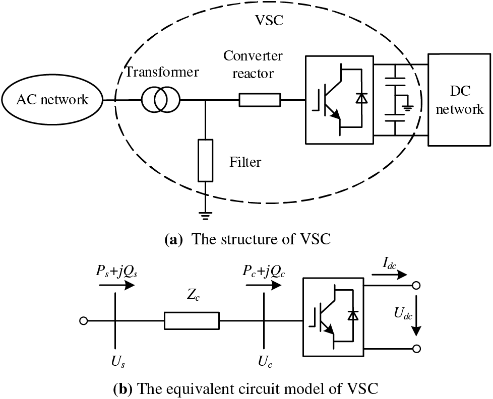
Figure 5: The structure of VSC and its equivalent circuit model

In Fig. 5, Ps and Qs are the active and reactive power on the AC side of the VSC; Us and Uc are the effective value of the line voltage on the AC side of the VSC and the line voltage on the converter side; Pc and Qc are the active and reactive power on the converter side; Udc is the DC side voltage; Idc is DC side current; Zc=Rc+jXc represents the equivalent impedance of the converter. If δs>δc, the converter runs in the rectified state, and if δs<δc, the converter runs in the inverter state. The figure shows that the power flow direction is positive.

It can be seen from the figure that the power flow constraints of VSC branches are as follows:

Ps−I2Rc=Pdc(34)

Qs−I2Xc=Qdc(35)

where I is the current flowing on the AC branch; Pdc is the active power transmitted by the converter to the DC system; Qc is the reactive power output of the converter.

In addition, the input active power Ps on the AC side of the converter, the active power loss Pc,loss of the equivalent resistance, the switching loss Ploss inside the converter, and the input active power Pdc on the DC side conform to the law of conservation of energy, which can be expressed as:

Ps=Pc,loss+Ploss+Pdc(36)

Pc,loss=Ps2+Qs2Us2Rc(37)

Ploss=a+bIc+cIc2(38)

Ic=Pc2+Qc23Uc(39)

Pdc=UdcIdc(40)

where Ic is the alternating current flowing through the inside of the converter; a, b and c are the loss coefficients that characterize different types of loss and are constants derived from practical experience, where a represents the inherent loss that is independent of Ic, b represents the loss that is proportional to Ic, and c represents the loss that is proportional to Ic square.

This paper employs a master-slave control strategy. Initially, a VSC is designated as the primary converter, implementing constant DC voltage control to guarantee system voltage stability. Subsequently, other VSCs are employed as slave converters, utilizing constant active power control to uphold consistent active power levels at nodes. The VSC control mode associated with this control strategy is illustrated in Fig. 6.

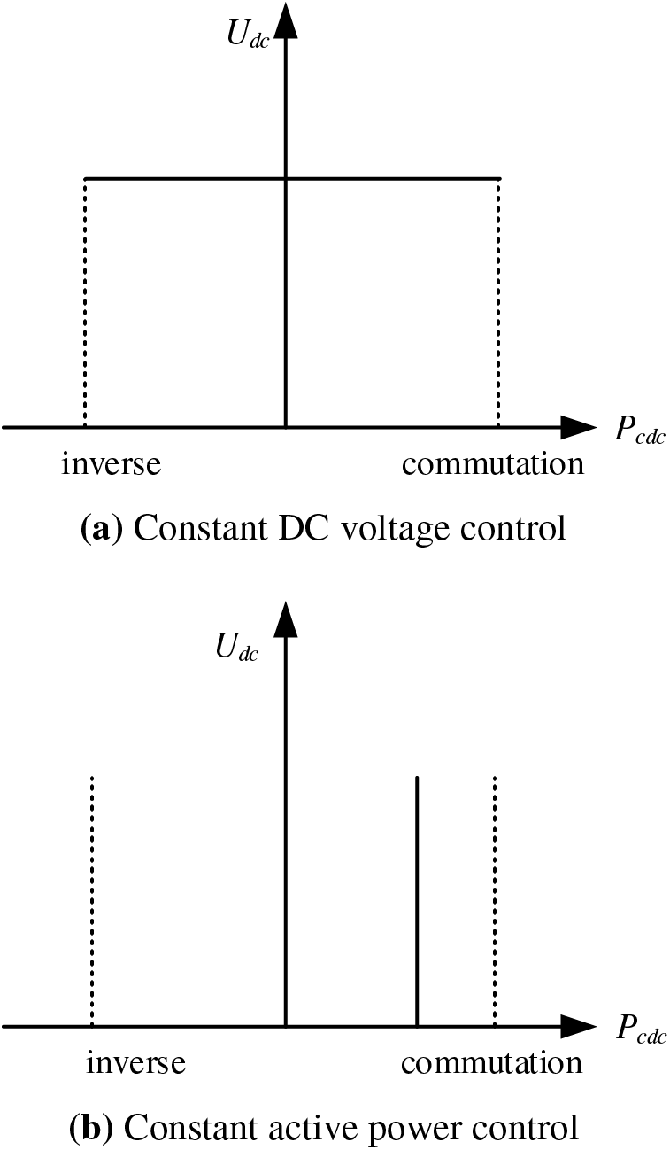
Figure 6: Two control modes of the master-slave control policy

(2) AC Power Flow Constraint

The nodes that are not connected to the VSC converter in the system are common, and the corresponding constraints are shown in Eqs. (41) and (42).

ΔP=Ui∑j=1NUj(Gijcos⁡θij+Bijsin⁡θij)(41)

ΔQ=Ui∑j=1NUj(Gijcos⁡θij−Bijsin⁡θij)(42)

where Ui and Uj are the node voltage of nodes i and j; θ is the phase Angle difference of nodes i and j.

For AC nodes that access VSC, the power injected by VSC at the AC side needs to be increased based on general nodes [25]. For example, the injected power at the node i of the flexible interconnected AC system includes the inflow of power supply and the outflow of load power, on this basis, it is also necessary to consider the active and reactive power of the converter into the AC system through the node i, as shown in Eqs. (43) and (44).

ΔPi=Ui∑j∈iUj(Gijcos⁡θij+Bijsin⁡θij)−(Pgi−Pli+Psi)(43)

ΔQi=Ui∑j∈iUj(Gijsin⁡θij−Bijcos⁡θij)−(Qgi−Qli+Qsi)(44)

where ΔPi is the unbalance of active power injected into node i; ΔQi is the unbalance of reactive power injected into node i; Pgi is the active power that the external power supply flows into the system through node i; Qgi is the reactive power that the external power supply flows into the system through node i; Pli is the active power flowing out of the system through the node i, which is the load active power; Qli is the reactive power that flows out of the system through the node i, which is the load reactive power; Psi is the active power that the converter flows into the AC system through node i; Qsi is the reactive power that the converter injects into the AC system through the node i.

(3) DC Power Flow Constraint

In contrast to the intricate steady-state power flow equations in AC power grids, DC power grids have a simpler set of equations. In DC power grids, there are no two-parameter variables like the phase angle of node voltage and reactive power flowing within the network. So, the steady-state power flow equations for DC power grids exclusively involve real variables, devoid of imaginary components. Due to the addition of a significant number of VSCs, the corresponding current constraints have been altered, and the underlying principles are similar to AC constraints.

ΔPdci=Udci∑j=1j≠indcGdcij(Udcj−Udci)−(Pc,dci+Pgdci−Pldci)(45)

where Pc.dci is the active power flowing into the DC side by the VSC converter through the node i; Pgdci is the active power that the external power supply flows into the DC side through the node i; Pldci is the active power that flows out of the DC network through the nodes i, which is the load power.

(4) Nodal Voltage Constraint

Ui,min≤Ui≤Ui,max(46)

where Ui,max and Ui,min are the upper and lower limits of the voltage of the node i, respectively.

(5) PV Output Constraint

0≤PPV(t)≤PPV,max(47)

where PPV(t) is the output power of PV during the period t; PPV,max is the upper limit of the output power of PV.

(6) Power Balance Constraint

Eq. (48) is the electrical equilibrium constraint of the system, and Eq. (49) is the hydrogen energy equilibrium constraint of the system.

Pload=PPV+PBT+PHFC−PEL(48)

PEL=PHFC+Pcf,in−Pcf,out(49)

where Pload is the electric load; PPV, PBT, PEL and PHFC are the output power of PV, BT, EL, and HFC, respectively; Pcf,in and Pcf,out are the charging and discharging power of HST, respectively.

3.3 Solution Procedure

This paper incorporates three objective functions. To enhance the visualization of optimization outcomes, we employ the non-dominated sorting genetic algorithm-II (NSGA-II) for solution optimization. This algorithm includes the elite strategy [26,27] and achieves the desired results through iterative optimization. Each objective is computed and presented individually, allowing the selection of the appropriate scheme by examining the trends within the final Pareto solution set.

The specific procedural steps in this paper can be summarized as follows:

(1) Determine the network structure of the flexible interconnection system, input the original data of the AC network and the DC network, as well as the population number and iteration times of the algorithm.

(2) According to the results of reference [4], distributed PV and HS are installed at the corresponding nodes.

(3) Determine control variables and objective functions.

(4) Encode the variables and generate the initial population randomly.

(5) The alternating iteration method is used to calculate the power flow results of the AC/DC hybrid distribution network, and three objective functions are calculated.

(6) The NSGA-II algorithm was used to solve the three objective functions iteratively.

(7) Determine whether the convergence condition of the iteration is met. If the condition is met, go to step (8); otherwise, go to step (5) and calculate again.

(8) Output the Pareto optimal solution set that meets the conditions, and the corresponding output status of load, PV, HS, etc.

Combined with the above steps, Fig. 7 illustrates the operational flowchart for a flexible interconnection distribution network that takes into account distributed PV and HS.

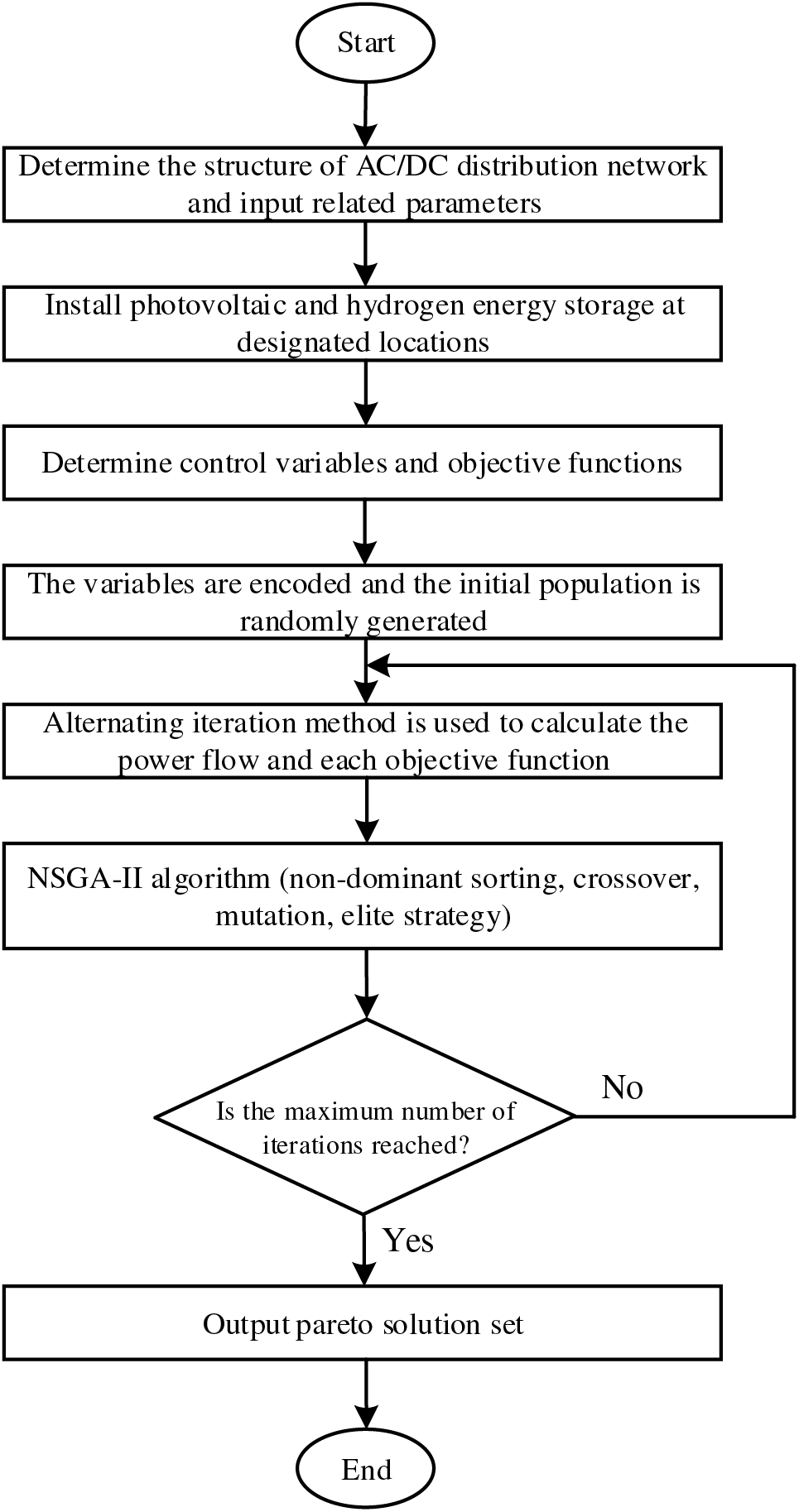
Figure 7: Operation flow

4  Case Studies

4.1 Test System Parameters

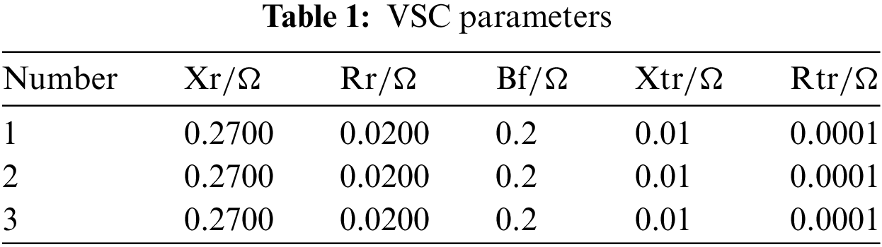
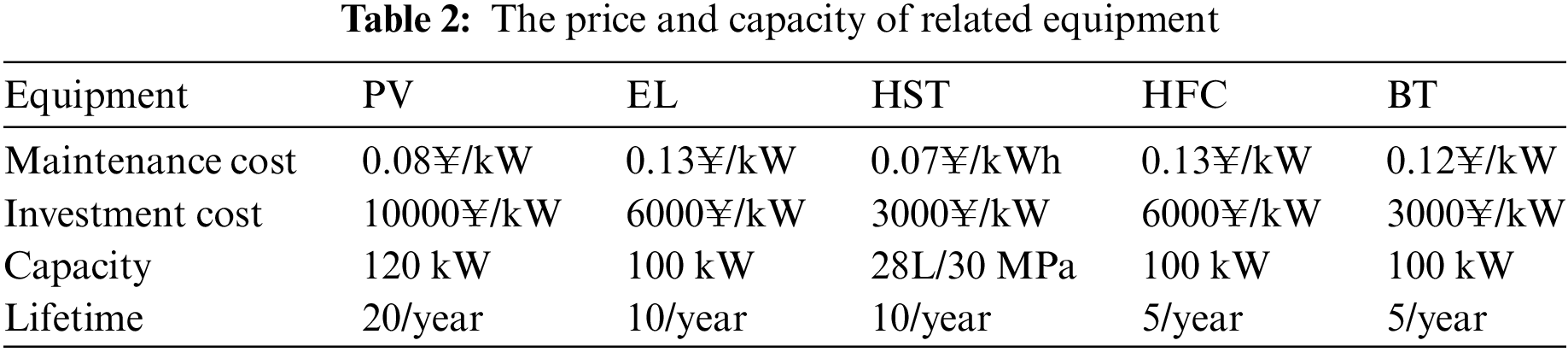
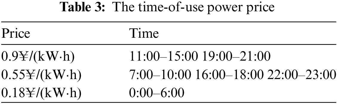
In the improved IEEE33 node system, converters VSC1, VSC2, and VSC3 have been introduced to transform it into an AC/DC hybrid distribution network. The AC terminals of these converters are linked to nodes 23, 29, and 17 of the AC distribution network, while the DC distribution network comprises three VSC DC terminals. Aside from the VSC ports, there are no other DC nodes, as depicted in Fig. 8. In this example, the reference power for the AC system is set at 10 MVA, with a reference voltage of 12.66 kV. For the DC system, the reference power is also 10 MVA, with a reference voltage of 10 kV. Detailed converter parameters are shown in Table 1, with LossA for all three inverters at 0.12, LossB at 0.029, and LossC at 0.00031. Furthermore, PV units have been installed at nodes 7, 10, 13, 14, 16, 18, 23, 26, and 31, and energy storage systems are situated at nodes 8, 11, 12, 19, 22, 27, 30, and 32. Reference prices for each of these devices are provided in Table 2 [4]. The NSGA-II algorithm employs a population size of 200 and a maximum iteration limit of 100 to achieve optimization. Additionally, Table 3 displays the time-of-use power prices.

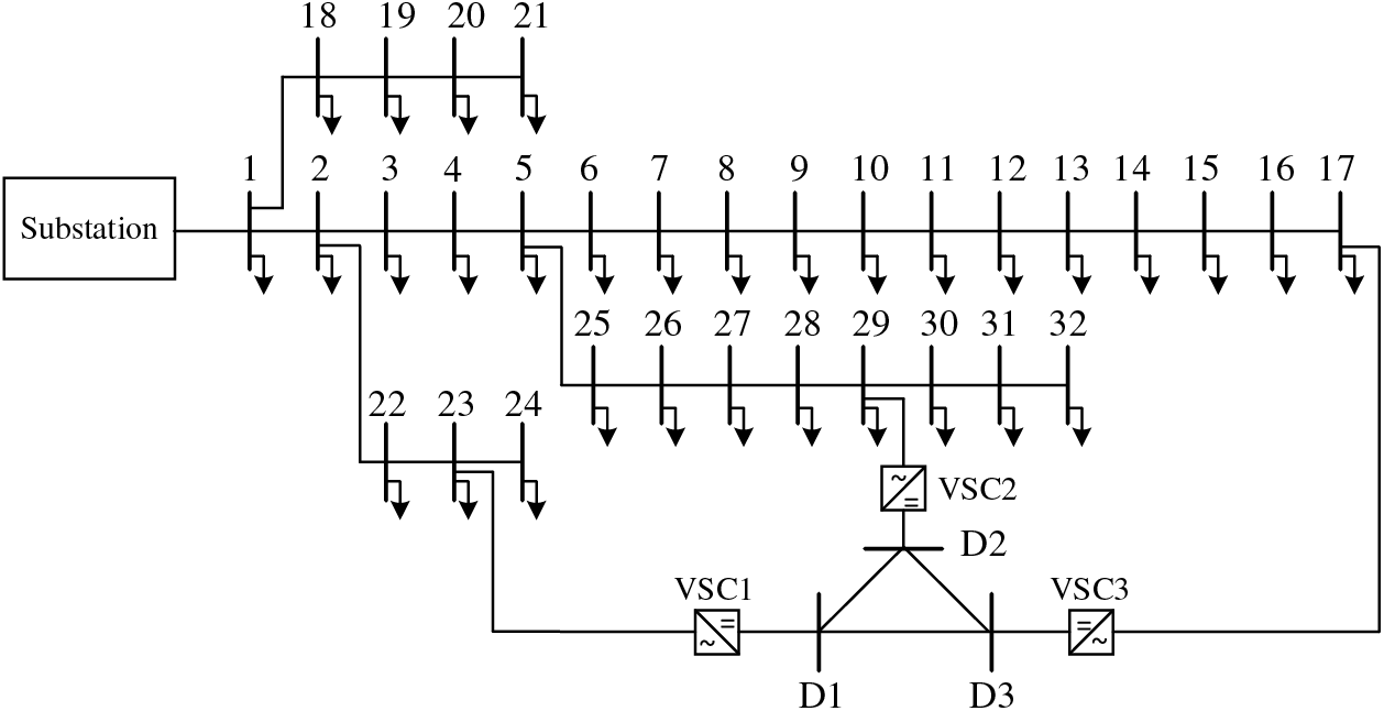
Figure 8: The improved IEEE33 node system

4.2 Simulation Analysis

4.2.1 Energy Storage System Operation Analysis

For the proposed flexible interconnection model, a representative 24-h PV output dataset is chosen, and the associated load fluctuations are computed, as illustrated in Fig. 9.

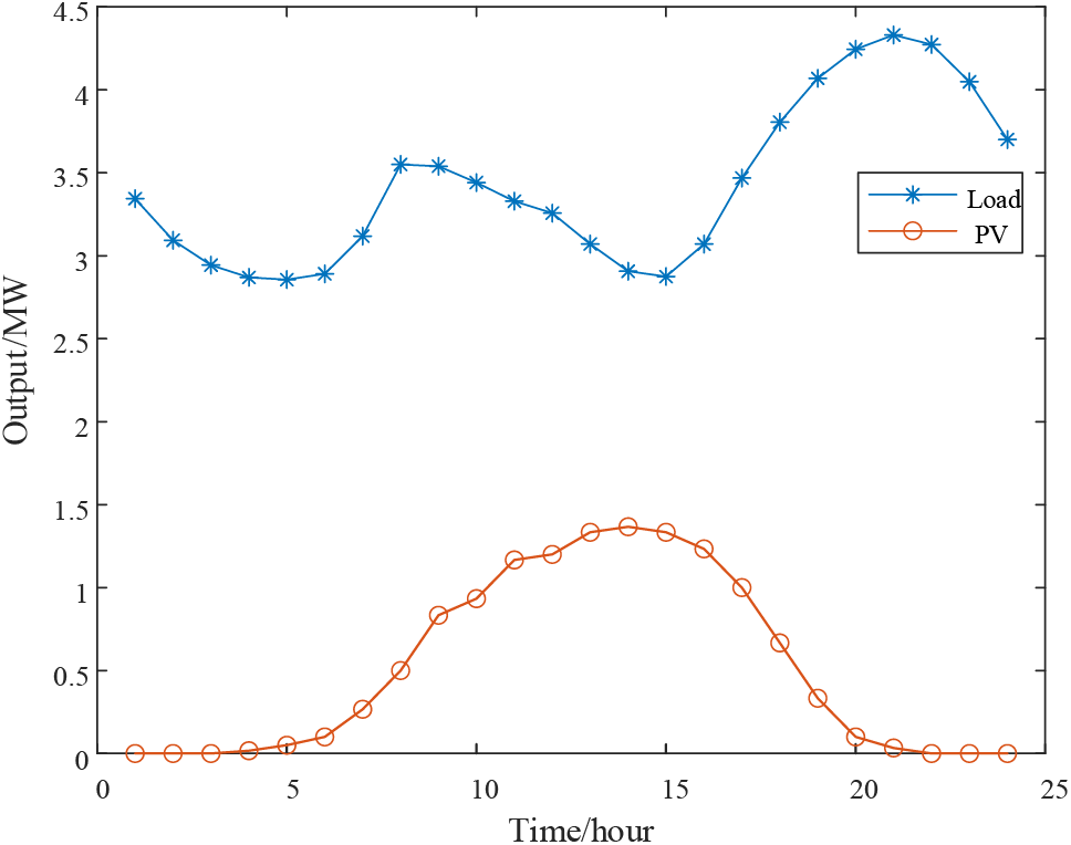
Figure 9: PV output and load fluctuation

The daily output of the conventional HS equipment is depicted in Fig. 10. From the figure, it can be observed that between 09:00 and 18:00, PV resources are abundant, resulting in PV output exceeding the load. The EL becomes operational during this period, converting surplus electrical energy into hydrogen and storing it within the HST. During the hours of 19:00–24:00 and 01:00–05:00, the intensity of light limits PV output, which falls to a lower level or even approaches zero, while the load surpasses the PV output. At this juncture, the hydrogen stored in the HST is reversed back into electrical energy through HFC, supplying the grid to compensate for the energy shortfall. Between 06:00 and 08:00, all the hydrogen gas in the HST has been depleted. During this period, the electric energy produced by the PV system is diminished and is not required for consumption, rendering the EL inactive. This observation underscores the effectiveness of the HS system in enhancing the consumption of distributed PV and optimizing system scheduling.

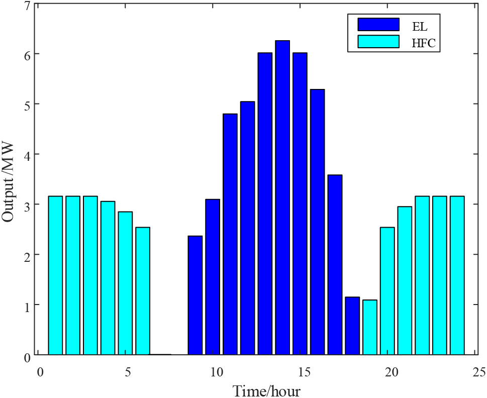
Figure 10: Conventional HS equipment output

Fig. 11 shows the 24-h capacity variation curve of the HST in the conventional HS system. From the figure, it can be observed that the HST capacity gradually decreases during 01:00–06:00 and 20:00–24:00, as the load levels are higher during this period, and there is less PV output, causing the HST to consume hydrogen to generate electricity. Meanwhile, during 10:00–19:00, when PV output is higher, the surplus electricity, after supplying the load, is redirected to the EL for hydrogen production, resulting in a gradual increase in the HST capacity. Between 6:00–9:00, the HST has already converted all the previously stored hydrogen into electricity, and with no new hydrogen replenishment, its capacity becomes zero.

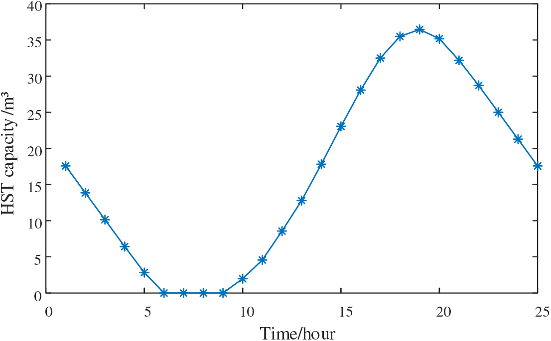
Figure 11: HST capacity change curve

Fig. 12 shows the PV output data and total load fluctuation of a certain node within a year. The peak of PV output is from August to October, and the trough period is January and December. Because the light intensity is high in summer and autumn, the PV power generation is large, and the light intensity is low in winter, and the PV power generation is less. The peak of load electricity consumption is from July to August and December, and the trough period is from February to March. Because the load demand is large in summer and winter, the electricity consumption is high, and the demand is less in spring and autumn, and the electricity consumption is less.

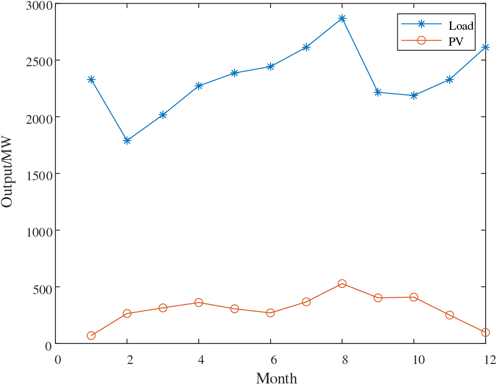
Figure 12: PV output data and total load fluctuation of a node

Fig. 13 shows the SHS charging and discharging status in one year. Combined with Figs. 12 and 13, it can be seen that in weeks 1–6 and 41–48, the PV output is low, while the load level is high due to heating and other reasons, the net load of the system is less than 0, and the energy storage system releases energy to supply the load. In weeks 7–16, the heating period ends, the load level decreases, the PV output begins to increase, there is excess electric energy after the distribution network operation, the net load of the system is greater than 0, and the energy storage system starts to charge. In weeks 17–24, the load continues to grow, the PV output fluctuates continuously, the load cannot be supplied in time, the grid has a shortage, the net load of the system is less than 0, and the energy storage system works to supplement the energy supply. In the 25–40 weeks, as the temperature rises, air conditioning and other equipment start, the load continues to increase, while the light intensity increases, the PV output rises, and there is still excess electricity after the supply load, the system net load is greater than 0, the energy storage system can be charged. It can be concluded that SHS can achieve scheduling optimization in units of years.

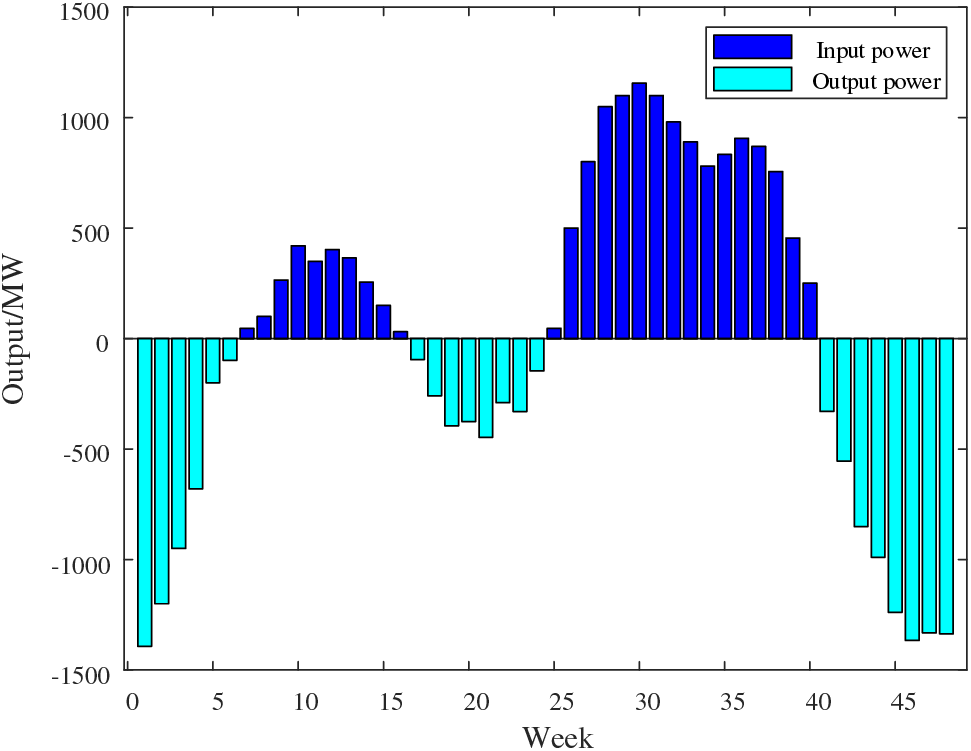
Figure 13: SHS charging and discharging state

Fig. 14 shows the charge and discharge status and capacity change of BT on a typical day per season. As can be seen from the figure, affected by the PV output and load demand, BT is charged in the low period of electricity consumption, and released in the peak period. The initial capacity of BT on the second day is the capacity of the last moment of the previous day, and the daily capacity change balance can achieve short-term optimal scheduling.

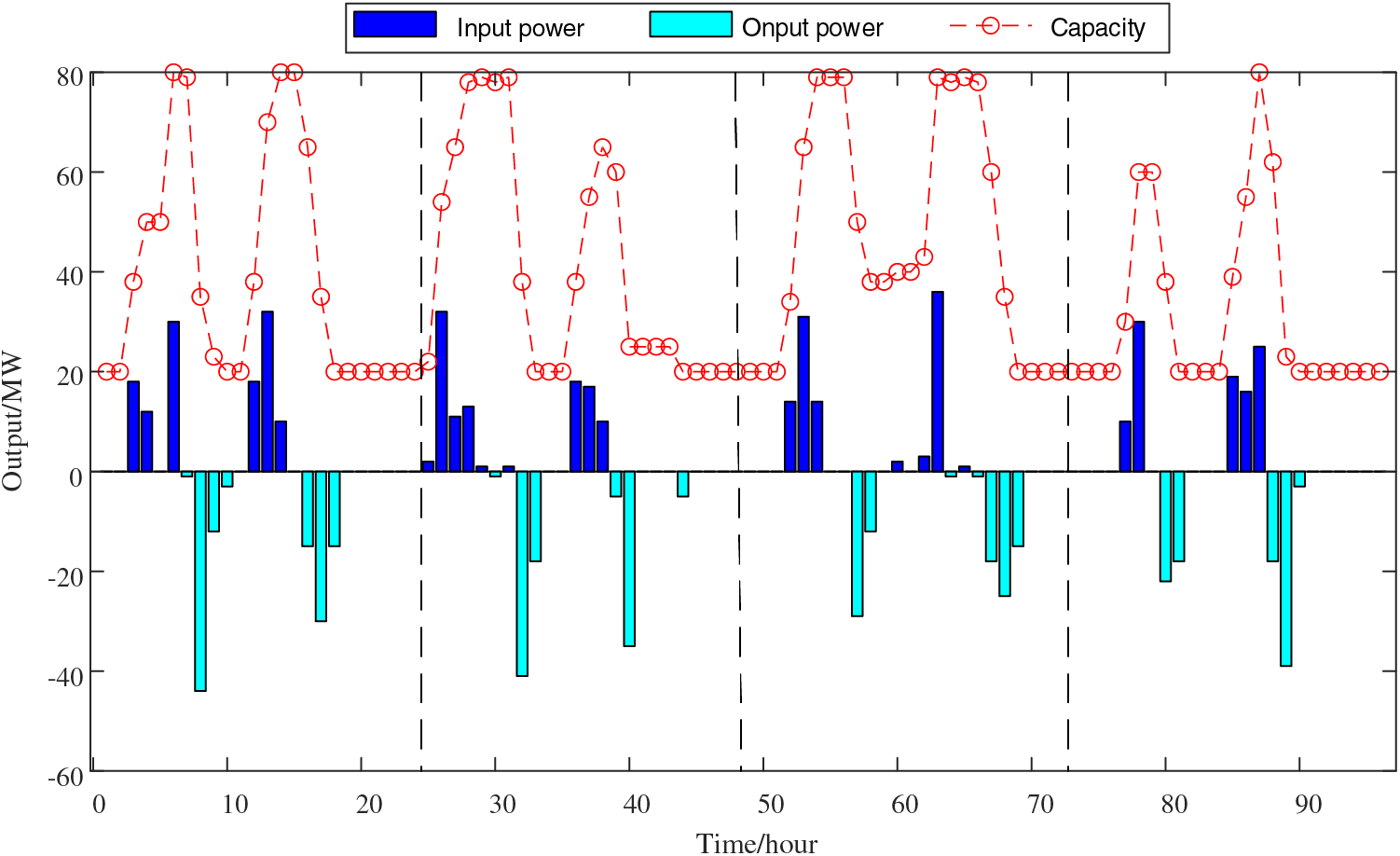
Figure 14: The charging and discharging state and capacity change of BT

4.2.2 Case Comparative Analysis

In addition, to verify the advantages of HS and flexible interconnection, the three objective functions proposed in this paper are divided into three different cases for comparative analysis:

Case 1: A distribution network system that considers PV, HS, and flexible interconnection;

Case 2: A distribution network system that considers PV and flexible interconnection without considering HS;

Case 3: A distribution network system that considers PV and HS without considering flexible interconnection.

The results of each case are shown in Figs. 15–17.

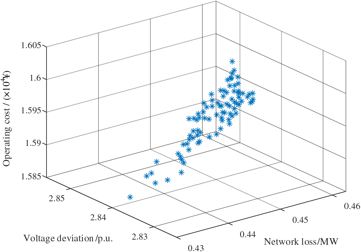
Figure 15: The objective function result of Case 1

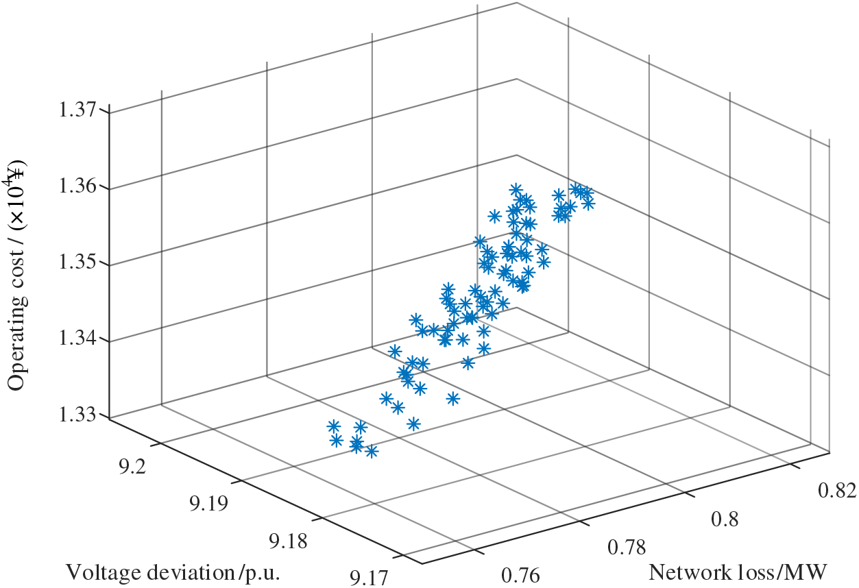
Figure 16: The objective function result of Case 2

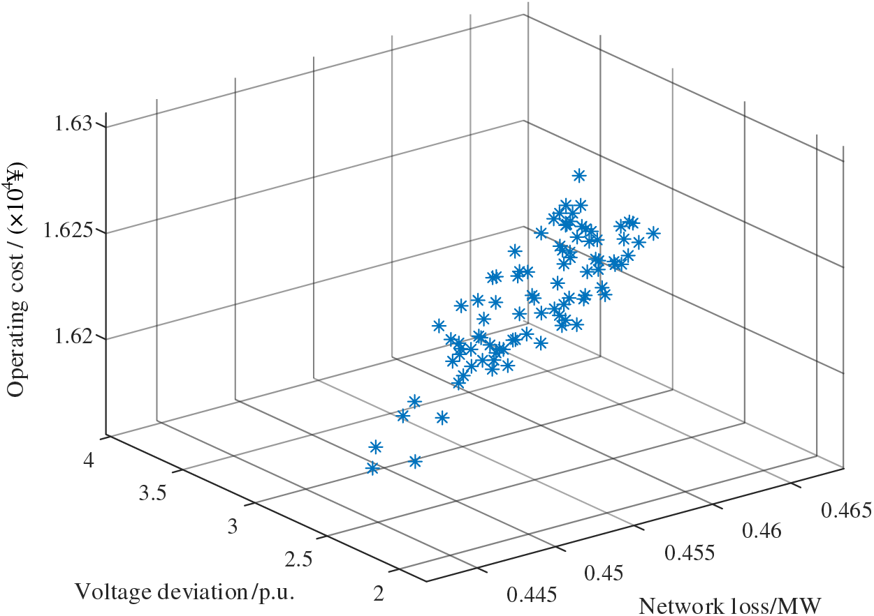
Figure 17: The objective function result of Case 3

From this, it can be seen that in Case 1, where HS and flexible interconnection are considered together, the system exhibits the lowest overall network losses, voltage deviations, and operating costs. In Case 2, in which HS is not considered, the operating costs are lower, but voltage deviations and network losses are significantly higher, which is detrimental to the stability of the power system. In Case 3, where flexible interconnection is not considered, the voltage deviations and network losses are similar to those in Case 1, but the operating costs are higher than in Case 1. The relevant data for these three objectives are presented in Table 4, Figs. 18 and 19.

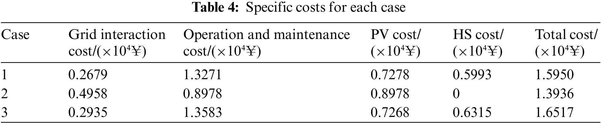
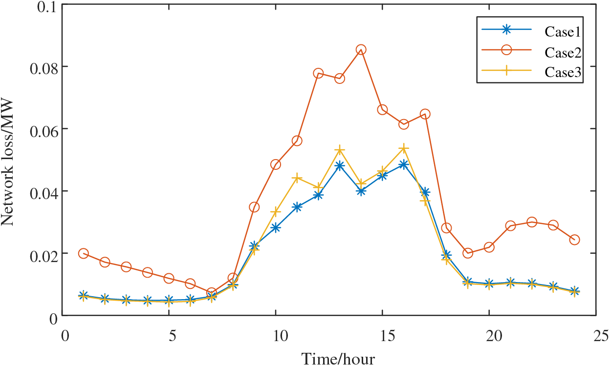
Figure 18: 24-h network loss in each case

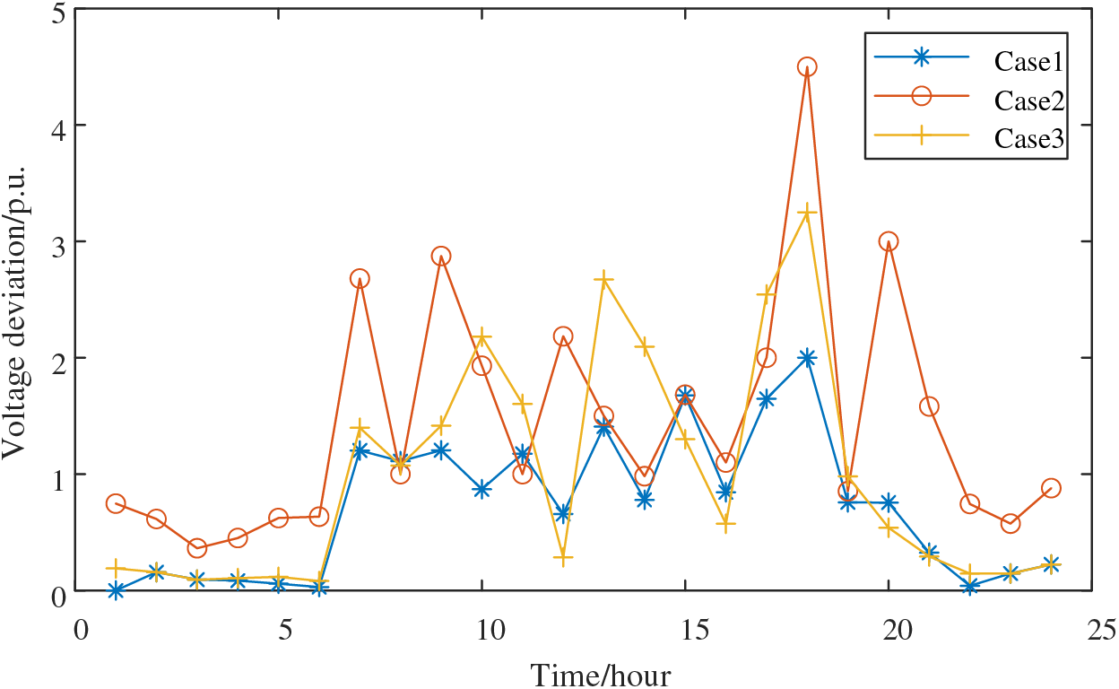
Figure 19: 24-h voltage deviation in each case

Table 4 shows the distinctions between the three cases. In Case 1, the addition of HS enables energy time transfer, while flexible interconnection facilitates energy circulation across various branches of the power grid. This effectively reduces grid interaction costs and minimizes the overall expenditure. In contrast, Case 2 lacks HS-related devices, leading to increased reliance on grid electricity during high-load periods. Although the equipment costs are lower, the expense associated with purchased electricity is higher. For Case 3, the absence of flexible interconnection necessitates a higher number of energy storage devices for adjustments, resulting in increased grid interaction costs. In comparison, the total cost of Case 1 is 3.55% smaller than that of Case 3.

Figs. 17 and 18 depict the network loss and voltage deviation of each scenario over 24 h, as exemplified in Fig. 9. Notably, between 07:00 and 20:00, significant system fluctuations occur due to changes in distributed PV output and network load. In this context, Case 1 consistently exhibits lower values in comparison to Case 2 and Case 3, indicating the best performance. Case 2, due to the absence of energy storage, displays the least capability to adapt to these fluctuations, resulting in the highest voltage deviation and network loss. Case 3’s network losses are similar in magnitude to those of Scenario 1, but it experiences higher voltage deviations at times 10, 13, 14, 17, and 18.

Based on the above analysis, it can be concluded that the conclusion that the operation of the distribution network system, which integrates PV and HS with flexible interconnection as seen in Case 1, is more stable and cost-effective.

4.2.3 Comparison of Different Algorithms

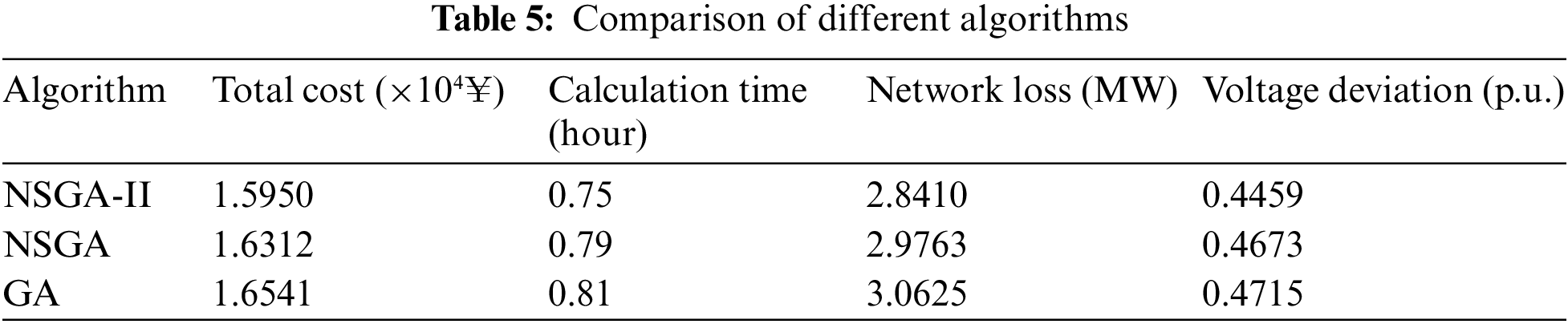
To verify the performance of the optimization algorithm used in this paper, the NSGA-II algorithm was compared with the NSGA algorithm and GA algorithm, and optimized under the condition of Case 1. The population size of all algorithms was set to 200 and the maximum number of iterations was set to 100. The comparison results are shown in Table 5. It can be seen that the total cost of the GA algorithm and NSGA algorithm is higher than that of the NSGA-II algorithm in this paper, while the calculation time of the NSGA-II algorithm is reduced by 5.3% and 8.1% compared with the NSGA algorithm and GA algorithm, respectively, and the network loss is reduced by 135.3 and 221.5 kW, respectively. Voltage deviation was reduced by 3.5% and 5.7%, respectively. Therefore, the NSGA-II algorithm adopted in this paper has a better calculation effect.

5  Conclusion

This paper establishes a flexible interconnection distribution network scheduling optimization model considering distributed PV and HS, comprehensively studies the impact of HS and flexible interconnection on the distribution network, and draws the following conclusions through numerical analysis and simulation verification:

(1) Combining SHS with short-term energy storage, this paper proposes a comprehensive energy storage system considering seasonal HS, which can realize the real-time energy supply and demand balance and the adjustment of seasonal fluctuations of renewable energy, ranging from a few minutes to a few months.

(2) The HS system established in this paper can realize the two-stage energy conversion from electricity to hydrogen to electricity, and its combination with distributed PV can effectively promote PV consumption, reduce the loss and voltage deviation of the distribution network during peak hours, and improve the power quality of the power system.

(3) In this paper, flexible interconnection technology is used to build the AC/DC hybrid distribution network, and the power flow in the system is regulated by VSC, which can save 3.55% of the cost and improve the economy of the power system when combined with distributed PV and HS systems.

(4) In this paper, the NSGA-II multi-objective optimization algorithm is used to solve multi-objective optimization problems to obtain uniformly distributed Pareto frontier, providing relatively complete and accurate information. In practical projects, decision-makers can get specific schemes according to the emphasis of different objectives.

The AC/DC hybrid distribution network system studied in this paper only represents the scheduling of a region in the time dimension, while HS can realize the energy interaction between different regions through hydrogen pipeline transportation and long-tube trailer transportation. In future work, the optimal scheduling method of SHS in the space dimension will be further explored to eliminate the imbalance between regions.

Acknowledgement: This paper is supported by the Science and Technology project of State Grid Jibei Electric Power Company Limited Smart Distribution Network Center (Research on Key Technologies of Flexible Interconnection in Low-Voltage Distribution Areas Considering Random Load Transfer).

Funding Statement: The authors received no specific funding for this study.

Author Contributions: The authors confirm contribution to the paper as follows: study conception and design: Yang Li, Zhaojian Jun; data collection: Zhaojian Jun, Xiaolong Yang; analysis and interpretation of results: Xiaolong Yang, He Wang and Yuyan Wang; draft manuscript preparation: Yang Li, He Wang and Yuyan Wang. All authors reviewed the results and approved the final version of the manuscript.

Availability of Data and Materials: The authors confirm that the data supporting the findings of this study are available within the article. The additional data that support the findings of this study are available on request from the corresponding author, upon reasonable request.

Conflicts of Interest: The authors declare that they have no conflicts of interest to report regarding the present study.

References

1. Mohamed, M. A., Almalaq, A., Abdullah, H. M., Alnowibet, K. A., Alrasheedi, A. F. et al. (2021). A distributed stochastic energy management framework based-fuzzy-PDMM for smart grids considering wind park and energy storage systems. IEEE Access, 9, 46674–46685. [Google Scholar]

2. Abdallah, W. J., Hashmi, K., Faiz, M. T., Flah, A., Channumsin, S. et al. (2023). A novel control method for active power sharing in renewable-energy-based micro distribution networks. Sustainability, 15(2), 1579. [Google Scholar]

3. Borousan, F., Hamidan, M. (2023). Distributed power generation planning for distribution network using chimp optimization algorithm in order to reliability improvement. Electric Power Systems Research, 217, 109109. [Google Scholar]

4. Bai, M., Tang, W., Tan, H., Gao, F., Yan, T. (2016). Optimal allocation of photovoltaic energy storage in urban distribution network based on virtual partition scheduling and two-layer planning. Electric Power Automation Equipment, 36(5), 141–148 (In Chinese). [Google Scholar]

5. Li, Y., Bu, F., Gao, J., Li, G. (2022). Optimal dispatch of low-carbon integrated energy system considering nuclear heating and carbon trading. Journal of Cleaner Production, 378, 134540. [Google Scholar]

6. Li, Y., Feng, B., Wang, B., Sun, S. (2022). Joint planning of distributed generations and energy storage in active distribution networks: A bi-level programming approach. Energy, 245, 123226. [Google Scholar]

7. Hamidan, M., Borousan, F. (2022). Optimal planning of distributed generation and battery energy storage systems simultaneously in distribution networks for loss reduction and reliability improvement. Journal of Energy Storage, 46, 103844. [Google Scholar]

8. Sun, E., Shi, J., Zhang, L., Ji, H., Zhang, Q. et al. (2023). An investigation of battery energy storage aided wind-coal integrated energy system. Energy Engineering, 120(7), 1583–1602. [Google Scholar]

9. Zhang, Z., Lv, Q., Zhao, L., Zhou, Q., Gao, P. et al. (2023). Research on optimal configuration of energy storage in wind-solar microgrid considering real-time electricity price. Energy Engineering, 120(7), 1637–1654. [Google Scholar]

10. Li, Y., Wang, B., Yang, Z., Li, J., Li, G. (2022). Optimal scheduling of integrated demand response-enabled community-integrated energy systems in uncertain environments. IEEE Transactions on Industry Applications, 58(2), 2640–2651. [Google Scholar]

11. Oh, M., Kim, B., Yun, C., Kim, C. K., Kim, J. et al. (2022). Spatiotemporal analysis of hydrogen requirement to minimize seasonal variability in future solar and wind energy in South Korea. Energies, 15(23), 9097. [Google Scholar]

12. Pan, G., Gu, W., Qiu, H., Lu, Y., Zhou, S. et al. (2020). Bi-level mixed-integer planning for electricity-hydrogen integrated energy system considering levelized cost of hydrogen. Applied Energy, 270, 115176. [Google Scholar]

13. Lu, M., Li, X., Li, F., Xiong, W., Li, X. (2023). Two-stage stochastic programming of seasonal hydrogen energy-mixing gas turbine system. Proceedings of the CSEE, 43(18), 6978–6992 (In Chinese). [Google Scholar]

14. Pan, G., Gu, W., Lu, Y., Qiu, H., Lu, S. et al. (2020). Optimal planning for electricity-hydrogen integrated energy system considering power to hydrogen and heat and seasonal storage. IEEE Transactions on Sustainable Energy, 11(4), 2662–2676. [Google Scholar]

15. Wang, X., Yang, W., Liang, D. (2021). Multi-objective robust optimization of hybrid AC/DC distribution networks considering flexible interconnection devices. IEEE Access, 9, 166048–166057. [Google Scholar]

16. Wang, X., Guo, Q., Tu, C., Li, J., Xiao, F. et al. (2023). A two-stage optimal strategy for flexible interconnection distribution network considering the loss characteristic of key equipment. International Journal of Electrical Power and Energy Systems, 152, 109232. [Google Scholar]

17. Gao, S., Liu, S., Liu, Y., Zhao, X., Song, T. E. (2019). Flexible and economic dispatching of AC/DC distribution networks considering uncertainty of wind power. IEEE Access, 7, 100051–100065. [Google Scholar]

18. Hu, R., Wang, W., Wu, X., Chen, Z., Ma, W. (2022). Interval optimization based coordinated control for distribution networks with energy storage integrated soft open points. International Journal of Electrical Power & Energy Systems, 136, 107725. [Google Scholar]

19. Shi, M., Zhang, J., Ge, X., Fei, J., Tan, J. (2023). Power optimization cooperative control strategy for flexible fast interconnection device with energy storage. Energy Engineering, 120(8), 1885–1897. [Google Scholar]

20. Yang, F., Sun, Q., Han, Q., Wu, Z. (2016). Cooperative model predictive control for distributed photovoltaic power generation systems. IEEE Journal of Emerging and Selected Topics in Power Electronics, 4(2), 414–420. [Google Scholar]

21. Zhang, W., Maleki, A., Rosen, M. A., Liu, J. (2019). Sizing a stand-alone solar-wind-hydrogen energy system using weather forecasting and a hybrid search optimization algorithm. Energy Conversion and Management, 180, 609–621. [Google Scholar]

22. Yilmaz, F., Ozturk, M., Selbas, R. (2020). Design and thermodynamic modeling of a renewable energy based plant for hydrogen production and compression. International Journal of Hydrogen Energy, 45(49), 26126–26137. [Google Scholar]

23. Kavadias, K. A., Apostolou, D., Kaldellis, J. K. (2018). Modelling and optimisation of a hydrogen-based energy storage system in an autonomous electrical network. Applied Energy, 227, 574–586. [Google Scholar]

24. Li, X., Guo, L., Li, Y., Hong, C., Zhang, Y. et al. (2018). Flexible interlinking and coordinated power control of multiple DC microgrids clusters. IEEE Transactions on Sustainable Energy, 9(2), 904–915. [Google Scholar]

25. Cai, H., Yuan, X., Xiong, W., Zheng, H., Xu, Y. et al. (2022). Flexible interconnected distribution network with embedded DC system and its dynamic reconfiguration. Energies, 15(15), 5589. [Google Scholar]

26. Verma, S., Pant, M., Snasel, V. (2021). A comprehensive review on NSGA-II for multi-objective combinatorial optimization problems. IEEE Access, 9, 57757–57791. [Google Scholar]

27. Pires, D. F., Antunes, C. H., Martins, A. G. (2012). NSGA-II with local search for a multi-objective reactive power compensation problem. International Journal of Electrical Power & Energy Systems, 43(1), 313–324. [Google Scholar]