
 Submit a Paper
 Propose a Special lssue
 Open Access
ARTICLE

Fault Distance Estimation Method for DC Distribution Networks Based on Sparse Measurement of High-Frequency Electrical Quantities
Key Laboratory of Modern Power System Simulation and Control & Renewable Energy Technology, Ministry of Education (Northeast Electric Power University), Jilin, 132012, China
* Corresponding Author: Shiqiang Li. Email:
Energy Engineering 2025, 122(11), 4497-4521. https://doi.org/10.32604/ee.2025.065244
Received 07 March 2025; Accepted 26 May 2025; Issue published 27 October 2025
 View Full Text
 Download PDF
Abstract
With the evolution of DC distribution networks from traditional radial topologies to more complex multi-branch structures, the number of measurement points supporting synchronous communication remains relatively limited. This poses challenges for conventional fault distance estimation methods, which are often tailored to simple topologies and are thus difficult to apply to large-scale, multi-node DC networks. To address this, a fault distance estimation method based on sparse measurement of high-frequency electrical quantities is proposed in this paper. First, a preliminary fault line identification model based on compressed sensing is constructed to effectively narrow the fault search range and improve localization efficiency. Then, leveraging the high-frequency impedance characteristics and the voltage-current relationship of electrical quantities, a fault distance estimation approach based on high-frequency measurements from both ends of a line is designed. This enables accurate distance estimation even when the measurement devices are not directly placed at both ends of the faulted line, overcoming the dependence on specific sensor placement inherent in traditional methods. Finally, to further enhance accuracy, an optimization model based on minimizing the high-frequency voltage error at the fault point is introduced to reduce estimation error. Simulation results demonstrate that the proposed method achieves a fault distance estimation error of less than 1% under normal conditions, and maintains good performance even under adverse scenarios.Keywords
The rapid development of renewable energy and power electronics technologies has led to increasing penetration of new energy sources and modern loads in power grids, thereby challenging the hosting capacity of traditional AC distribution networks. In contrast, DC distribution networks demonstrate significant advantages through high-efficiency power transmission, conversion capabilities, and seamless integration with renewable energy and energy storage systems [1–3]. However, DC systems face a critical challenge: the rapid rise of fault currents with complex characteristics, which poses substantial threats to system reliability [4]. Consequently, rapid and accurate fault localization in DC distribution networks becomes essential for fault isolation and system restoration [5].
Existing fault location methods for DC distribution networks can be divided into two categories based on their accuracy attributes and functional requirements: Fault section location and fault distance estimation [6].
The fault section location involves determining the specific line segment or region where the fault occurs. The goal is to quickly identify and isolate the fault area, ensuring the restoration of power to non-fault areas and the stable operation of the system. This technology is mainly divided into two types: passive and active. The passive section location constructs a discrimination model based on the characteristics generated during a fault to locate the fault section. Reference [7] implements section judgment through analysis of the energy polarity of DC current signals; Reference [8] proposes a frequency-hopping discrete Fourier transform algorithm to identify DC microgrid faults based on bus current harmonic characteristics; Reference [9] uses multi-band zero-mode current fuzzy entropy and zero-mode current concavity fluctuation features for radial distribution network monopole fault feeder identification. For large-scale, complex topological DC distribution networks with limited measurement point configurations, Reference [10] employs compressed sensing technology for bipolar short-circuit fault location. Active fault section localization, on the other hand, is achieved by injecting signals and analyzing the responses. For example, this can involve changing the MMC (Modular Multilevel Converter) control strategy [11] and injecting square waves, injecting fault detection signals and measuring currents at specific frequencies at both ends of the line [12], or using dual active bridge converters [13] to inject specific frequency harmonics for fault section location.
Fault distance estimation is used to determine the distance between the fault point and a reference point. The aim is to reduce fault troubleshooting time and improve power supply reliability. The research methods for fault distance estimation in DC distribution networks can be divided into three types: wave-based methods, injected signal-based methods, and fault transient information analysis methods. The wave-based method estimates fault distance based on the time difference and wave speed of fault transient waves propagating along the line. Some literature uses improved gray correlation analysis [14] and high-pass filtering algorithms [15] to improve the accuracy of distance estimation. The injected signal method involves injecting additional signals and analyzing their propagation information to perform distance estimation. For instance, Reference [16] uses a probe unit to generate voltage signals of arbitrary amplitude and frequency to locate faults, while Reference [17] utilizes MMC active signal injection and constructs parameter identification equations for fault localization. Fault analysis methods involve detecting electrical data and solving the fault location through circuit equations, such as calculating transient energy for distance estimation [18] or using the least squares method [19] to estimate the line resistance to the fault point and compare it to the actual line resistance to calculate the fault location. With the development of machine learning technology, this technology is also applied in the field of fault ranging in DC distribution networks [20]. Reference [21] utilizes the feature matrix to train the LSTM model to achieve fault ranging in DC microgrids.
In summary, current fault section localization and fault distance estimation methods for DC distribution networks are predominantly limited to systems with relatively simple network topologies. Considering the constraints of cost-effectiveness and practicality, it is often infeasible to deploy measurement devices comprehensively across all nodes or lines in large-scale and topologically complex DC distribution networks. This significantly limits the direct applicability of many existing methods in such networks. Although certain localization techniques based on compressed sensing can achieve fault section identification under sparsely deployed measurement configurations, their accuracy remains insufficient to meet the stringent requirements of fault distance estimation. Therefore, realizing accurate fault distance estimation in large-scale DC distribution networks with complex topologies and sparse measurement configurations remains a critical challenge that needs to be addressed.
To tackle this issue, this paper proposes a fault localization method for DC distribution networks based on sparsely sampled high-frequency electrical quantities. The main contributions are as follows:
(1) Accurate fault distance estimation is achieved for multi-node, complex-topology DC distribution networks under limited measurement node deployment conditions.
(2) A fault localization model is constructed within the compressed sensing framework, and a Pearson correlation coefficient-based generalized orthogonal matching pursuit algorithm (PGOMP) is proposed, significantly improving the accuracy of faulted line identification.
(3) A fault distance estimation method based on high-frequency electrical quantities at two remote terminals is developed, enabling distance estimation even when measurement nodes are not directly installed at both ends of the faulted line.
(4) A fault distance optimization model is introduced based on the minimum error in high-frequency voltage at candidate fault points, effectively reducing localization error and improving estimation accuracy.
The remainder of this paper is organized as follows: Section 2 briefly reviews conventional short-circuit fault distance estimation principles. Section 3 describes the proposed method for locating short-circuit faults in DC distribution networks. Section 4 introduces the dual-terminal-based fault distance estimation method and the fault distance optimization model. Section 5 presents simulation-based validations.
2 Analysis of Fault Characteristics in DC Distribution Networks
When a short-circuit fault occurs in a DC distribution network, the voltage at the fault point exhibits step characteristics, and the fault signal contains full-frequency domain information. Fig. 1 shows the time-frequency characteristics of the fault voltage. In the low-frequency band, the amplitude is larger but exhibits stronger nonlinearity and poorer stability. Conversely, in the high-frequency band, the amplitude variation is smaller with superior stability. Therefore, high-frequency band information is adopted for fault distance estimation [10,22].
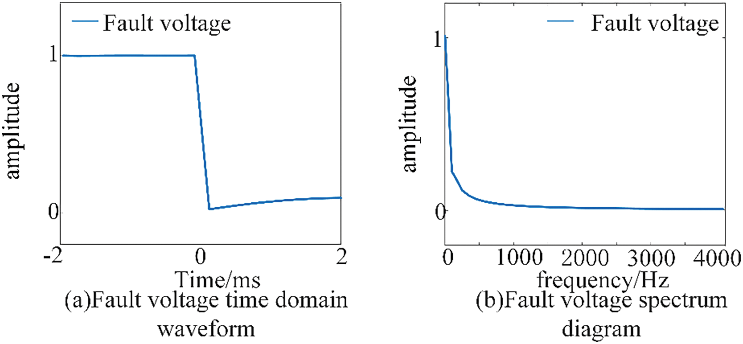
Figure 1: Time-frequency characteristic diagram of voltage sag during short-circuit fault, (a) fault voltage time domain waveform, and (b) fault voltage spectrum diagram
As shown in Fig. 2, the equivalent additional network of a short-circuit fault in a DC distribution network can be modeled as a high-frequency signal source injected at the fault point, containing rich multi-frequency components. To simplify the analytical process, this paper selects a specific frequency
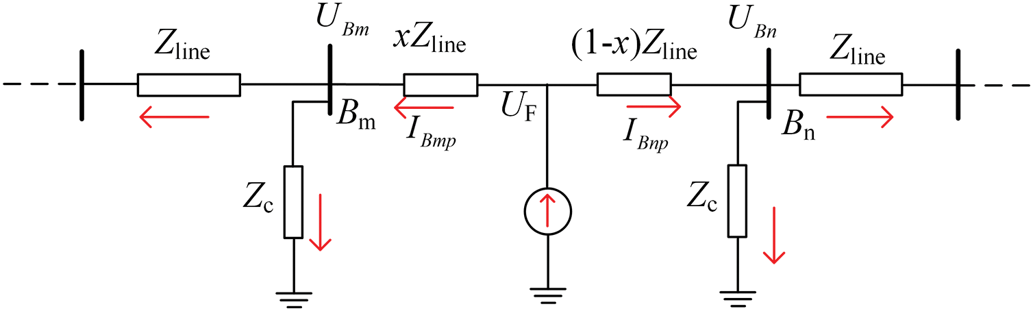
Figure 2: High-frequency additional network diagram for short-circuit fault
In Fig. 2, UF represents the fault source high-frequency voltage, Zline is the equivalent impedance of the DC line, Zc is the equivalent impedance of the converter, and x is the fault distance, i.e., the proportion of the fault point’s distance from the reference node along the total length of the line. UBm and UBn represent the fault high-frequency voltages on buses Bm and Bn, respectively.
The relationship between high-frequency electrical quantities and the fault distance is expressed by Eq. (1) in Fig. 2. Given the high-frequency voltage measurements UBm and UBn at adjacent nodes, and the fault high-frequency current injected into the line, the fault distance x can be calculated using Eq. (2), which enables fault distance estimation.
When this method is applied to a multi-node complex DC distribution network, high-frequency measuring devices must be installed at each node to perform fault distance estimation. However, due to the cost and practical limitations of equipment deployment, it is challenging to equip the entire network with measurement devices. This presents a technical challenge for fault distance estimation across the entire network. Therefore, this study will further discuss in subsequent sections how fault distance estimation can be achieved for a multi-node complex DC distribution network under conditions where the number of measurement devices is limited.
3 Fault Line Localization Method in DC Distribution Network
The localization of fault lines is a prerequisite for obtaining the electrical quantity information at both ends of the faulted line to achieve fault distance estimation. This section will explore how to accurately locate the faulted line in a DC distribution network under sparse measurement point configurations, based on compressed sensing technology.
3.1 Voltage Equation of the Fault High-Frequency Component Node
As shown in Fig. 3, the fault point in a DC distribution network short circuit can be considered as a fault high-frequency current source. Zc is the converter’s high-frequency equivalent impedance, Zline is the line’s high-frequency equivalent impedance, and If is the injected high-frequency fault current source [10].
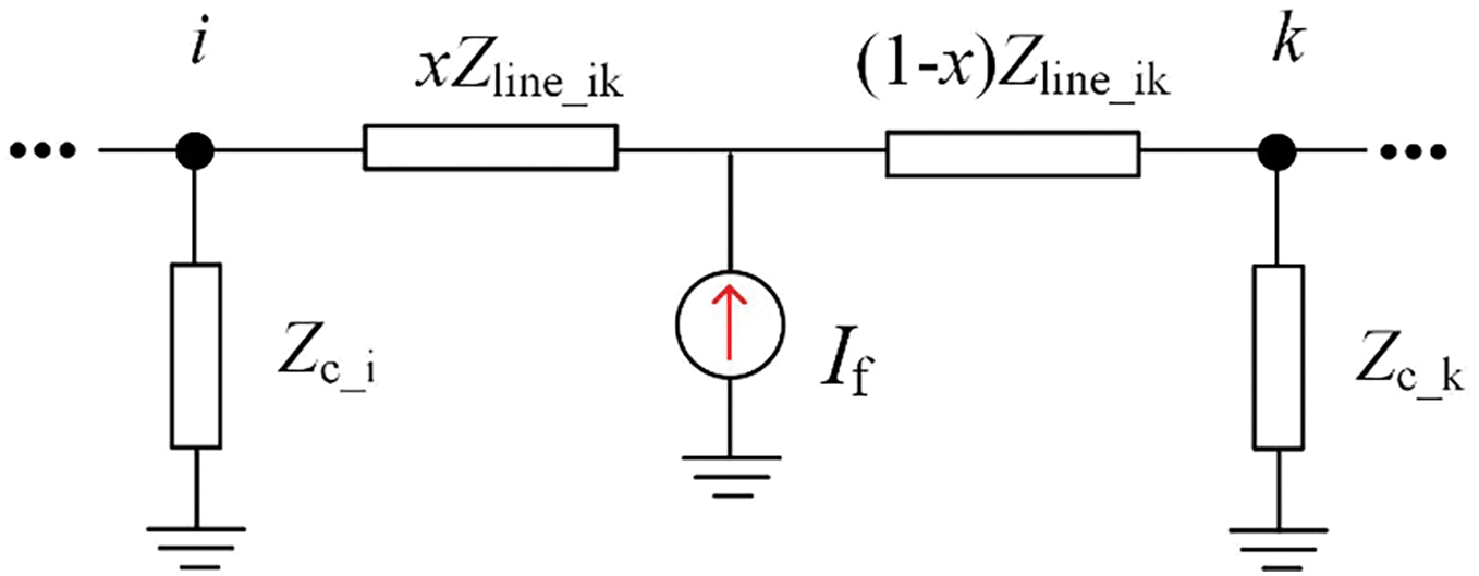
Figure 3: High-frequency network diagram for line fault analysis
But when a fault occurs on the line between nodes i and k in the distribution network, the fault cannot be directly represented by the high-frequency current vector I at the nodes. Therefore, the fault current source on the line is equivalently transferred to the two adjacent nodes, as illustrated in Fig. 4.

Figure 4: Equivalent network diagram for line fault analysis
The fault line localization method is based on the node high-frequency voltage equation. Consider a DC distribution network system with N nodes, where only M nodes (M ≪ N) are equipped with measurement devices under a sparse measurement configuration. Based on the dominant imaginary part characteristic of the system impedance under high-frequency conditions, the absolute value fault high-frequency node voltage equation can be established as follows [23].
In the equation, the high-frequency fault current vector
Eq. (4) represents an underdetermined system of equations, which will have an infinite number of solutions. Therefore, compressed sensing techniques are required to solve this underdetermined system in order to obtain a sparse solution and locate the faulted line.
3.2 Fault Line Localization Method Based on Compressed Sensing
The sparse representation problem in compressed sensing involves reconstructing the target signal b using the compressed signal Y and the observation matrix
In Eq. (5):
To locate short-circuit fault lines in DC distribution networks using compressed sensing methods, the model in Eq. (6) can be established:
In this equation, y,
The sensing matrix used in this paper is the node impedance matrix, where columns exhibit strong correlations. This necessitates a reconstruction algorithm with high discriminative capability. Therefore, the Pearson correlation coefficient is introduced to replace the inner product used in the greedy iterative algorithm of traditional compressed sensing, representing the similarity between the atom
The steps of the proposed PGOMP are as follows:
Step 1: Given the sensing matrix
Step 2: Compute the Pearson correlation coefficients between the residual
Step 3: Compute the sparse vector
Step 4: Compute the new residual vector
Step 5: If the iteration error reaches the predefined threshold, output the reconstructed vector.
Based on the above compressed sensing algorithm, fault line location is achieved by solving the node fault high-frequency voltage equation through the following steps:
(1) Construct the high-frequency impedance matrix according to the DC distribution network topology and line parameters, and obtain the measurement matrix
(2) Use wavelet transform to extract the high-frequency voltage signal
(3) Input sets of
4 Fault Distance Estimation in DC Distribution Networks Based on Dual-Terminal High-Frequency Electrical Quantities
After locating the faulty line, the high-frequency voltage and current values at the line’s terminal nodes can be indirectly acquired using high-frequency electrical quantities from upstream and downstream measurement points, combined with high-frequency impedance characteristics and voltage-current relationships. This enables fault distance calculation, thereby achieving fault distance estimation in DC distribution networks.
4.1 The Theory of Fault Distance Estimation in DC Distribution Networks
When a fault occurs on a line in the grid, the high-frequency fault signals propagate as shown in Fig. 5. In this figure, Zline represents the high-frequency impedance of the line, Zc_i is the equivalent ground component impedance of the faulted network at node i, and Ni refers to node i. Uf is the voltage generated by the fault source at the fault point.

Figure 5: High-frequency signal propagation diagram for fault analysis in the DC distribution network
In Fig. 5, if the fault occurs on line line_K and the measurement devices are installed at nodes NK and NK+1, high-frequency electrical quantities such as ilK+1, irK, uK and uK+1 can be directly obtained. Fault distance estimation can then be performed using Eq. (2). However, it is not guaranteed that the faulted line endpoints coincide with the measurement nodes. In this case, the high-frequency voltages and currents from the measurement nodes need to be used to indirectly estimate the electrical quantities at the faulted line endpoints.
For the fault scenario shown in Fig. 5, if the measurement device is installed at node NM−1, the high-frequency fault current irM−1 through line_M−1 and the fault high-frequency voltage uM−1 at node NM−1 can be obtained. Based on this, the fault high-frequency voltage uM at the upstream node NM of node NM−1 and the fault current irM through the upper-level line line_M can be estimated as follows:
By rearranging Eqs. (8) and (9), the following equation is obtained:
Therefore, when the fault high-frequency current and voltage of the current-level line and node are known, the fault high-frequency current and voltage of the upstream line and node can be recursively obtained using Eq. (10), thereby indirectly obtaining irK and uK, as shown in Eq. (11):
As shown in Fig. 5, based on the high-frequency electrical quantities irK and uK measured on the right side of the fault point, the expression for the fault source high-frequency voltage, derived from the downstream high-frequency electrical quantities, is given by Eq. (12).
Similarly, by considering the high-frequency fault current ilK flowing leftward through line line_K and the fault high-frequency voltage uK+1 at node NK+1, the fault source high-frequency voltage can be calculated using the upstream measurement node’s high-frequency voltage and current data following a principle similar to that of Eq. (11). Thus, based on the fault point’s high-frequency electrical quantities ilK and uK+1, as well as the data from the upstream measurement node, the fault source high-frequency voltage can be estimated, as shown in Eq. (13).
By computing the high-frequency electrical quantities from either the upstream or downstream lines and nodes, the theoretical values of the fault source high-frequency voltage should be consistent, which enables the fault distance x to be determined using Eq. (14).
Fig. 6 illustrates the theory of the fault distance estimation method. Thus, by utilizing the fault high-frequency voltage and high-frequency current measured by a limited number of devices installed on the DC distribution network, and given that the system parameters are known, precise localization of the DC distribution network short-circuit fault point has been achieved.

Figure 6: Schematic diagram for fault location based on dual-terminal high-frequency electrical quantities
4.2 Fault Distance Estimation Optimization Algorithm Based on Minimum Fault Point High-Frequency Voltage Error
Normally, the fault distance xt calculated at each time point t using the aforementioned method should be equal. However, due to the interference of background harmonics and measurement noise, errors exist between xt and the true fault distance. To reduce these errors, this paper employs data from multiple time points to calculate the fault distance and performs a comprehensive analysis of the resulting sets to obtain an optimal solution, thereby achieving precise fault distance estimation. The specific steps are as follows:
(1) Acquisition of Multiple Sets of Fault Distances: Based on the faulted line localization results, the two corresponding measurement points from the upstream and downstream sides are selected, and their high-frequency voltage and current data are extracted for each time point during the 2 ms fault period. Then, using the method described in Section 3.1, L sets of fault distance values xt are obtained for each time point t.
(2) Elimination of Outlier Fault Distances: Given that the fault distance results within the time window should be similar and distributed near the actual fault distance, the Z-score method is applied to identify and remove outliers from the multiple sets of distance measurements, thereby reducing their influence on the overall result. The Z-score is calculated using Eq. (15):
For each
(3) Optimization of Fault Distance Estimation Based on Minimum Fault Point High-Frequency Voltage Error: Incorporating the high-frequency electrical quantities corresponding to the P sets of fault distances at their respective time points, an optimization formula for fault distance estimation based on the minimum fault point high-frequency voltage error is proposed, as shown in Eq. (16):
In Eq. (16),
Eq. (16) comprehensively integrates the high-frequency electrical quantities from the remaining effective time points to compute the fault distance, thereby yielding the most accurate distance estimation. The optimized result from Eq. (16) is then output as the final fault distance estimation, completing the fault distance estimation process.
4.3 Fault Distance Estimation Flow
The flowchart of fault distance estimation is shown in the Fig. 7. And the fault distance estimation method for DC distribution networks based on sparse high-frequency measurements is as follows:

Figure 7: Schematic diagram for fault location based on dual-terminal high-frequency electrical quantities
(1) Fault Line Localization: Extract high-frequency voltage data from all measurement points during the 2 ms fault period. Then, apply compressed sensing theory to solve Eq. (3) to locate the short-circuit fault line.
(2) Distance Candidate Generation: Select the nearest upstream and downstream measurement points of the fault line. Extract their high-frequency voltage and current data at each time point within the 2 ms window. Using these data, calculate L sets of fault distances according to Eqs. (11)–(14).
(3) Optimal Distance Determination: Compute the Z-score values of the L sets of fault distances and compare them with a preset threshold to filter out P sets of valid fault distances. Select the high-frequency electrical quantities corresponding to these valid fault distances at each time point. Then, perform optimization using Eq. (16) to obtain the final estimated fault distance xf.
5.1 DC Distribution Network Simulation Model
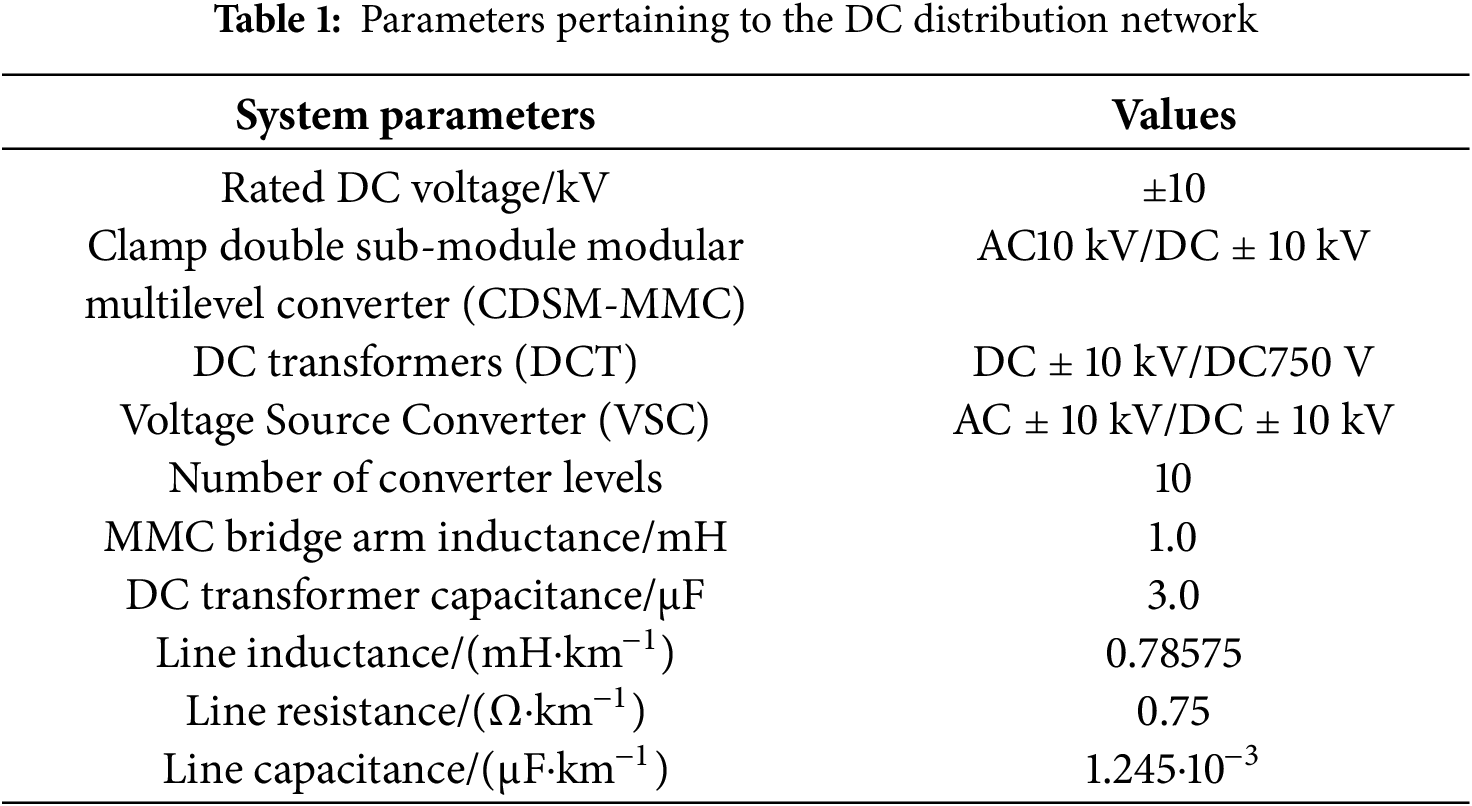
To validate the correctness and effectiveness of the proposed fault distance estimation method in multi-node complex-topology DC distribution networks, an IEEE 33-node DC distribution system shown in Fig. 8 was implemented on the PSCAD simulation platform. This system achieves flexible AC/DC interconnection through a Modular Multilevel Converter (MMC). Photovoltaic (PV) units and DC loads are connected to the network via DC transformers, while AC loads are integrated through Voltage Source Converters (VSCs). Detailed parameters of lines and converters are provided in Table 1.

Figure 8: The improved IEEE 33-Node simulation system
In this study, measurement devices are deployed at a total of 9 nodes as illustrated in the figure. These devices are capable of measuring high-frequency voltage at the nodes and high-frequency current on adjacent lines, thereby fulfilling the requirements of the proposed method. During the fault localization process, the extracted high-frequency signals operate at 1500 Hz, with a data sampling frequency of 10 kHz.
5.2 Verification of Fault Distance Estimation Method
To accurately evaluate the performance of the fault distance estimation method proposed in this paper, the relative error δ the fault distance is defined as follows:
where: xactual is the actual fault distance, xcalculation is the estimated fault distance, and Len is the total length of the line.
To validate the proposed fault distance estimation method, a pole-to-ground fault with a transition resistance of 0.1 Ω was set at a relative distance of 0.4 from node i on line L30–31.
First, the faulted line is determined by extracting the high-frequency voltage data from all measurement points in the DC distribution network during the fault period, and by using compressed sensing techniques to reconstruct the fault high-frequency current vector within a 2 ms window. As shown in Fig. 9, the reconstructed high-frequency current vector exhibits significantly high values at node numbers 30 and 31, from which the faulted line L30–31 is identified.

Figure 9: Reconstructed Current Vector for the fault on line L30–31
Next, based on the determined faulted line, the two measurement nodes closest to the upstream and downstream ends—nodes 28 and 32—were selected. The fault high-frequency voltage and current data extracted from these two nodes were then used to perform dual-end fault distance estimation. During the fault of line L30–31 (the fault starts at t = 1 s), the waveforms of the absolute values of fault high-frequency current and voltage measured by measuring nodes 28 and 32 are shown in Fig. 10.

Figure 10: Reconstructed current vector for the fault on line L30–31. Among them, (a,b) respectively show the high-frequency voltage and high-frequency current waveforms measured at node 32 during the fault period, (c,d) respectively show the high-frequency voltage and high-frequency current waveforms measured at node 28 during the fault period
Subsequently, based on the measured fault high-frequency voltage and current at each time point, the fault distance was estimated using the fault distance estimation method proposed in this paper, yielding L groups of fault distance values. The Z-score for each fault distance was also calculated. The fault distances computed at each time point are illustrated in Fig. 11, where the fault distances marked in red correspond to Z-score values that exceed the preset threshold.

Figure 11: Calculated fault distances at various time points
Finally, by filtering out the valid fault distance data corresponding to the time points and inputting them into the minimum error-based fault distance model for resolution, a fault distance of 0.3961 was obtained, with a relative error of only 0.39%. This experimental result validates the effectiveness and accuracy of the proposed fault distance estimation method.
5.3 Fault Location Results under Different Influencing Factors
5.3.1 Impact of Different Faulted Lines
To validate the feasibility and accuracy of the fault distance estimation method proposed in this paper across various regions of the DC distribution network, short-circuit faults with a transition resistance of 0.1 Ω were imposed on representative lines in each region at different positions xactual = 0.2, 0.4, and 0.6 for performance validation. The fault distance estimation results are shown in Tables 2 and 3. (Fault distance refers to the relative distance from the fault point to node i on the faulted line Li–j).
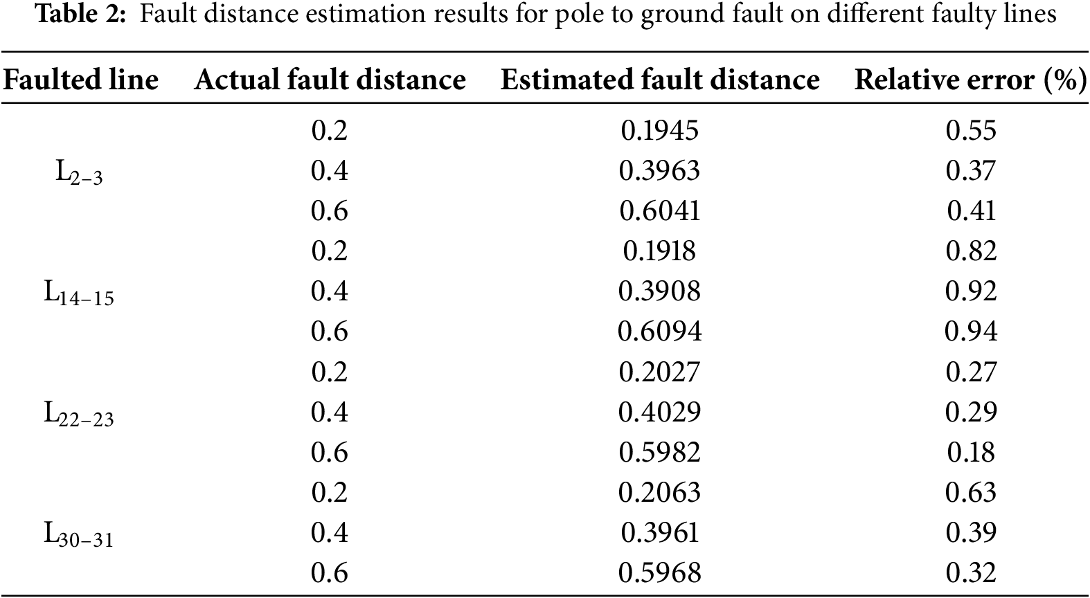
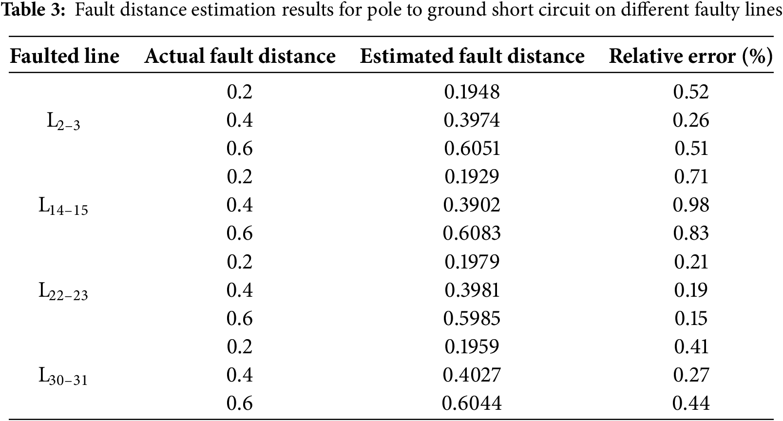
Tables 2 and 3 present the fault distance estimation results for four lines in the DC distribution network under short-circuit fault conditions. Among them, Line L22–23 exhibits a smaller estimation error due to the closer proximity of its terminal nodes to the measurement nodes. This phenomenon indicates that the estimation accuracy is influenced by the distance between the measurement points and the faulted line. Notably, the proposed algorithm consistently maintains a relative estimation error within 1% across different faulted lines, demonstrating its high accuracy in fault distance estimation.
5.3.2 Influence of Different Transition Resistors
To verify the proposed fault distance estimation method’s tolerance to transition resistance, tests were conducted using different values of transition resistance. The estimation results are presented in Tables 4 and 5.

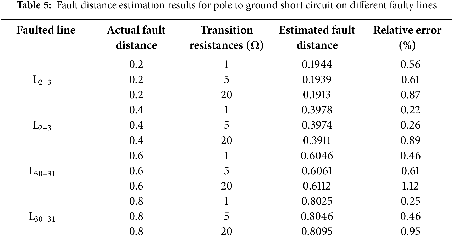
As evidenced by the results presented in Tables 4 and 5, it can be seen that the distance measurement scheme proposed in this paper can still accurately and reliably calculate the fault location even with transition resistance. As the transition resistance increases, the relative error tends to increase. This is because the increase in transition resistance will reduce the degree of voltage drop at the fault point, thereby reducing the equivalent high-frequency fault characteristics.
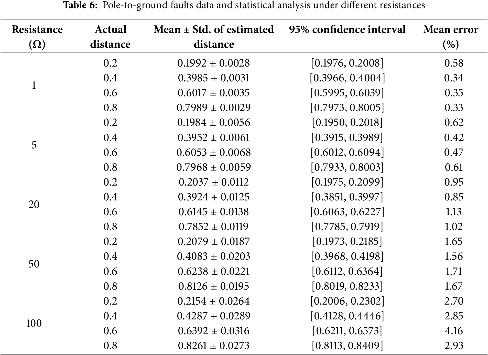
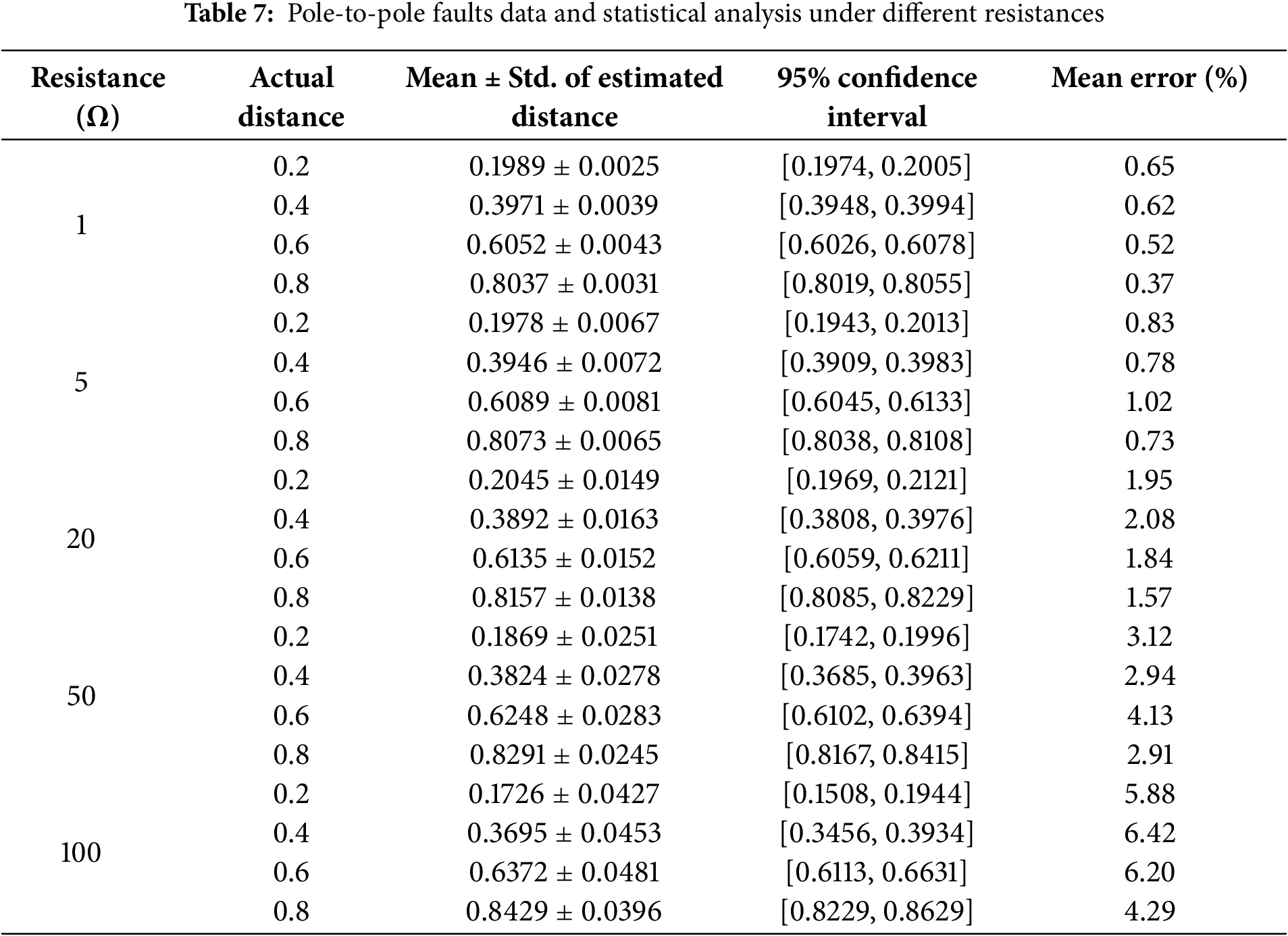
In addition to the existing results, supplementary fault distance estimation experiments were conducted on 48 equidistant points (divided into five sections) across 12 lines between nodes N1–N5 and N5–N32. Faults were simulated under different transition resistances. The results are shown in Tables 6 and 7.
5.3.3 Influence of Different Noise
The data collected by simulation models is under ideal operating conditions, but in actual engineering operations, the collected data is inevitably mixed with noise of different components, which can affect the fault location results. This article added a certain degree of Gaussian white noise to the simulated sampling data of fault line L10–11, and set the noise intensity signal-to-noise ratio to 50–30 dB. The fault location results and positioning errors are shown in Tables 8 and 9.
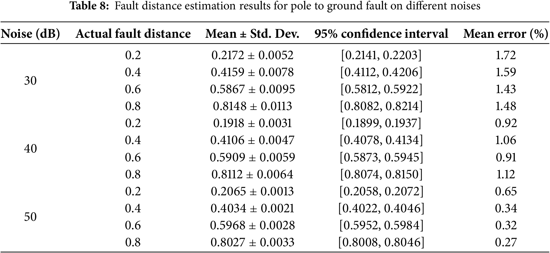
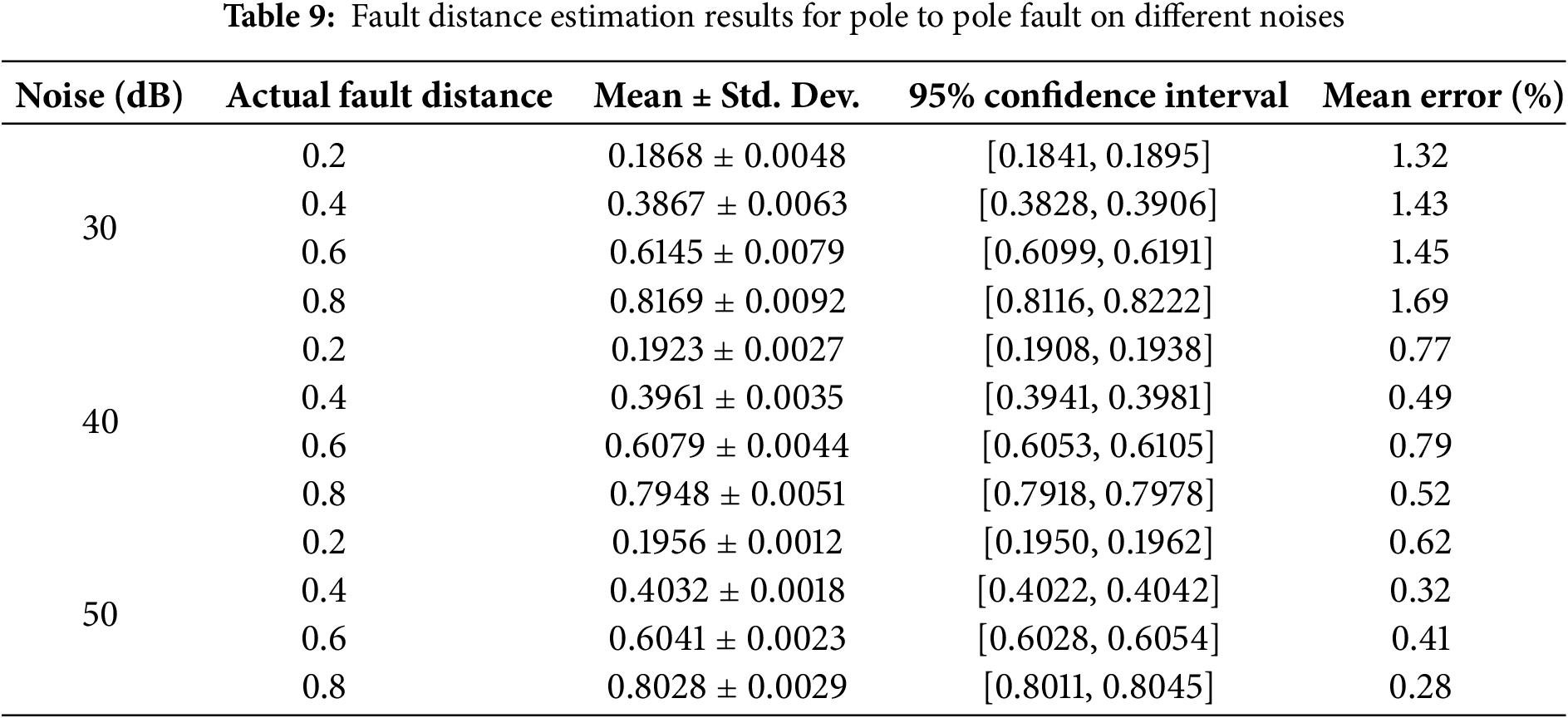
As shown in Tables 8 and 9, when 50 or 40 dB noise is added, the method proposed in this paper can still maintain a small fault distance measurement error, while the error becomes larger after the noise reaches 30 dB. However, this paper introduces an optimization step based on the minimum fault distance error in fault distance measurement, which to some extent reduces the impact of noise.
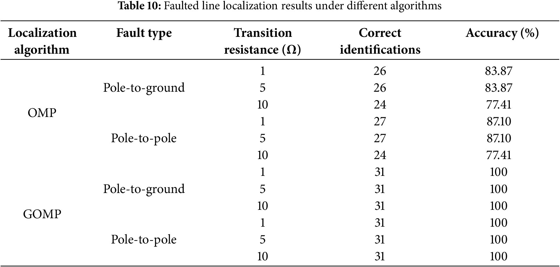
1. Comparison of Faulted Line Identification Accuracy Between PGOMP and Classical OMP Algorithms
In this section, we compare the performance of the proposed PGOMP algorithm with the classical Orthogonal Matching Pursuit (OMP) algorithm in terms of faulted line identification accuracy. The comparison focuses solely on faulted line localization accuracy, as fault line identification and fault distance estimation are relatively independent processes.
Table 10 presents the faulted line identification results for both pole-to-ground and pole-to-pole faults across 31 branches under various transition resistance conditions. As can be seen, the proposed PGOMP algorithm significantly outperforms the classical OMP algorithm in all scenarios. It achieves 100% accuracy across all tested conditions, demonstrating its superior robustness and reliability.
It is worth noting that accurate faulted line localization is a prerequisite for fault distance estimation. Without first identifying the correct faulted line, any subsequent distance estimation would be meaningless. This further highlights the critical importance of the proposed method.
2. Ablation Study on Fault Distance Estimation
To assess the effectiveness of the minimum error optimization module, an ablation analysis was performed. This module comprises two components: “Outlier removal from fault distance results”, and “Optimization of fault distance estimation based on the minimum high-frequency voltage error at the fault point.”
Four experimental configurations were designed, as Table 11 shown below:
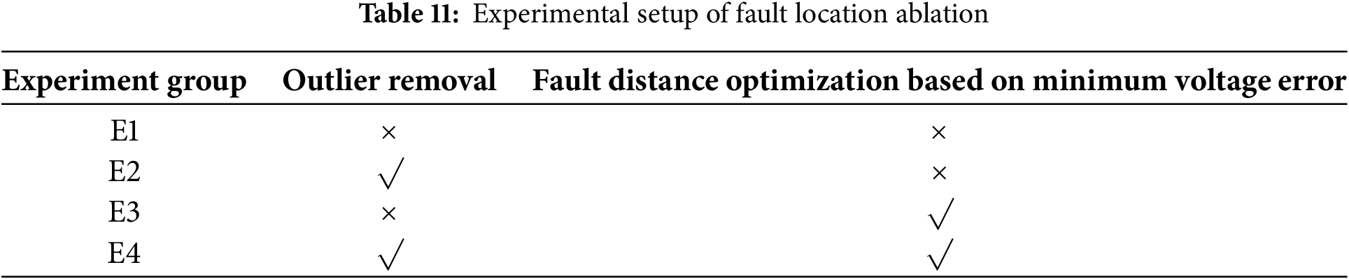
Outlier removal refers to the use of the Z-score method to detect and eliminate anomalous distance estimates. Fault distance optimization involves applying the method defined by Eq. (17), which minimizes the high-frequency voltage error at the fault point. In the absence of this optimization, the final fault distance is computed by averaging the estimates.
Pole-to-ground faults were simulated at 124 points (five equal divisions per line) across 31 lines in a DC distribution network, with a transition resistance of 0.1 Ω. The results under each experimental setting are presented in Table 12.
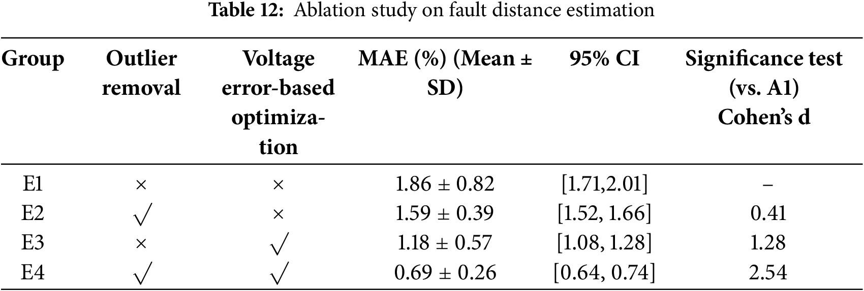
The above results and analysis demonstrate that both the outlier removal and the fault distance optimization based on minimum high-frequency voltage error significantly contribute to the reduction of estimation error. Specifically, outlier removal enhances the stability of the proposed algorithm by eliminating abnormal distance estimates, while the voltage error-based optimization significantly improves the accuracy of fault distance estimation.
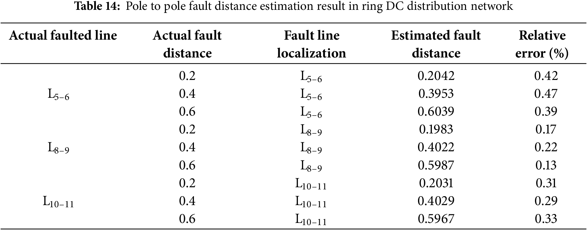
5.5 Analysis of Ring Distribution Network
In order to verify the feasibility and accuracy of the proposed fault location method across different regions of the DC distribution network, short-circuit faults with a transition resistance of 1 Ω are introduced at various locations along the ring network as shown in the Fig. 12. This serves to evaluate the method’s adaptability to other network topologies.
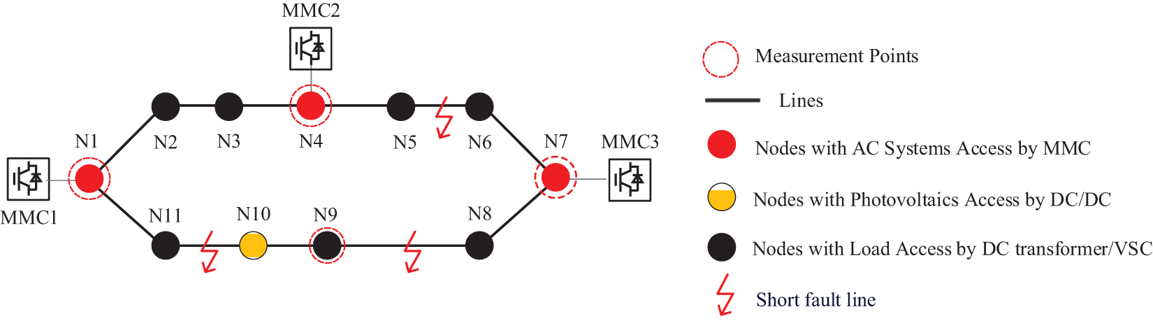
Figure 12: Topology of ring DC distribution network
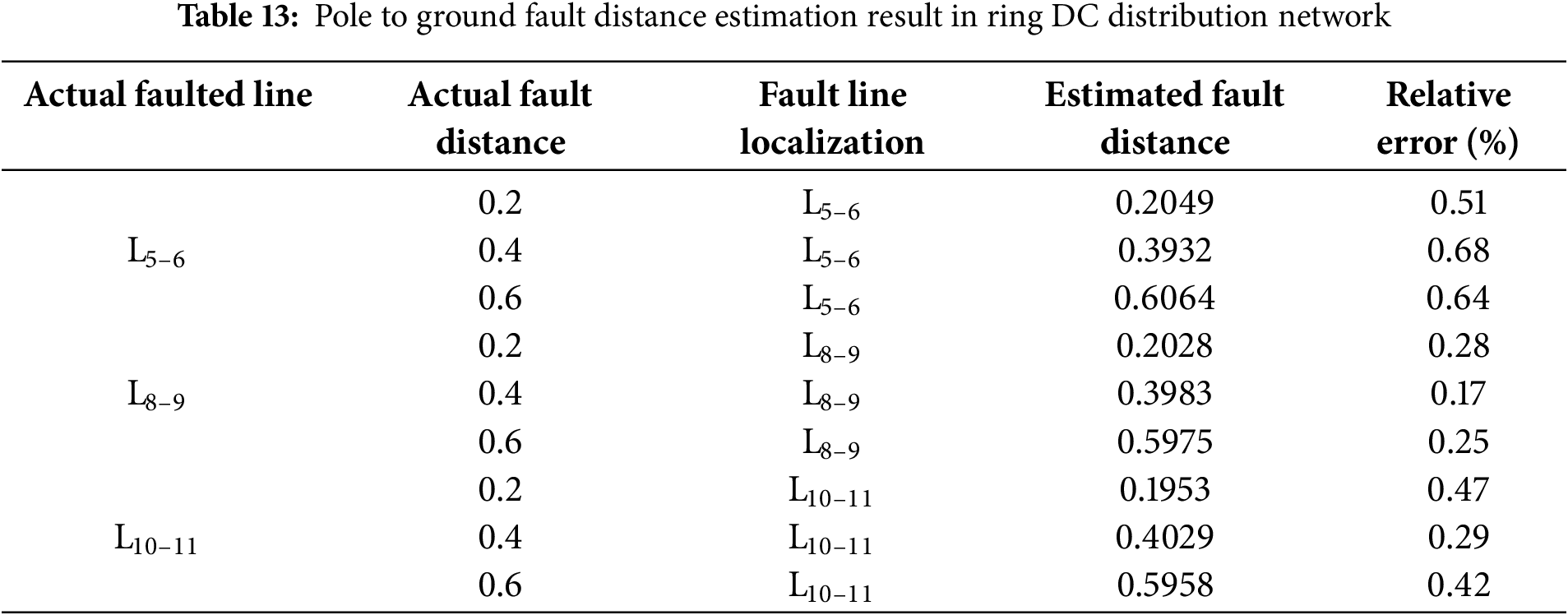
Tables 13 and 14 show the results of fault distance estimation for the ring network. The results indicate that the proposed algorithm can accurately identify the faulted line and estimate the fault distance with low error in ring-structured DC distribution networks, demonstrating its strong adaptability to different network topologies.
5.6 Comparison of the Proposed Method with Other Existing Methods
5.6.1 Comparison of Simulation Results between the Proposed Method and Existing Methods
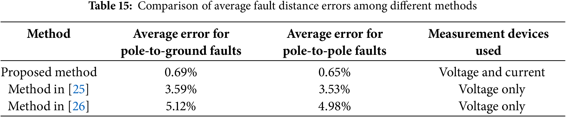
To verify the effectiveness of the proposed fault distance estimation principle and optimization algorithm, different methods were applied to estimate fault distances in a DC distribution network. The experiment considered short-circuit faults with a transition resistance of 0.1 Ω at various positions along line L30–31 (xactual = 0.2, 0.4, 0.6, 0.8) to evaluate fault distance estimation performance and compare errors between methods.
As shown in Table 15, the proposed method achieves average location errors of 0.69% and 0.65% under pole-to-ground and pole-to-pole faults, respectively. In contrast, the method in [25] exhibits higher errors of 3.59% and 3.53%, while the method in [26] shows even larger deviations of 5.12% and 4.98%. It is noteworthy that both [25,26] rely solely on voltage measurements, whereas the proposed method leverages both voltage and current information, contributing to its enhanced accuracy. Based on the comparison results, although the improved sparse measurement-based fault distance estimation method proposed in this paper requires more measurement devices than the other two sparse measurement approaches, the introduction of high-frequency current measurements significantly reduces the fault location error compared to the others. These results clearly demonstrate the comparative advantage of the proposed approach in terms of location precision under various fault types.
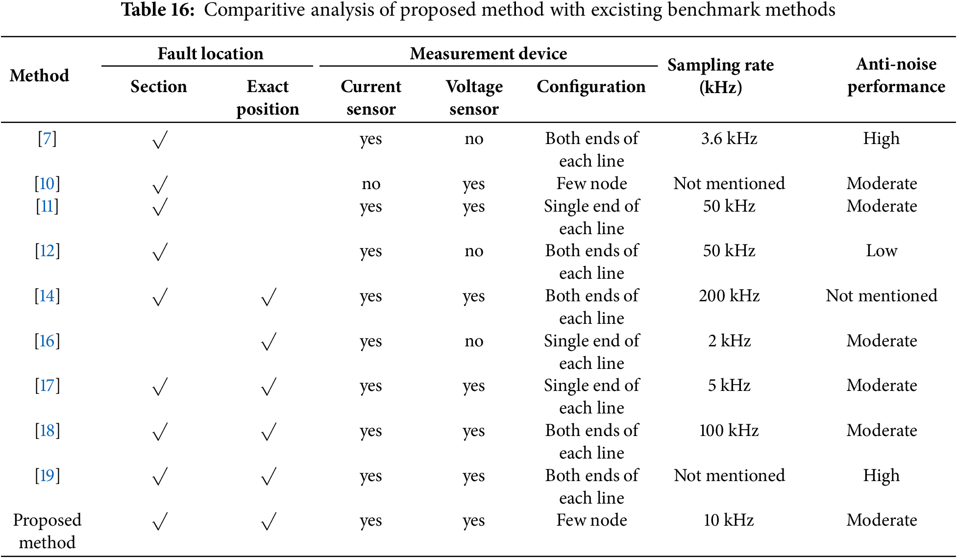
5.6.2 Comprehensive Comparison Study with Existing Methods
A comparative evaluation between the proposed method and several existing fault localization techniques is presented in the Table 16, focusing on key performance indicators such as localization capability, measurement device configuration requirements, sampling rate demands, and noise resistance. Compared with traditional methods, the proposed fault localization strategy demonstrates several notable advantages. First, in terms of localization functionality, the methods presented in [7,10–12] are limited to fault section identification and are unable to determine the exact fault location. In contrast, the proposed method enables accurate calculation of the precise fault point. Second, regarding measurement configuration, the proposed method overcomes the typical reliance on single-end or double-end measurements along the line, as commonly required by existing techniques. Instead, it only requires measurement devices to be sparsely deployed at a limited number of nodes. This greatly enhances the proposed method’s adaptability to complex topologies in multi-node DC distribution networks and improves the cost-effectiveness of the measurement system. Finally, in terms of functionality, the proposed method operates with a relatively low sampling frequency compared to existing approaches. Moreover, benefiting from the incorporated fault distance optimization mechanism, the system exhibits superior noise immunity, further enhancing its applicability in practical engineering scenarios.
To address the challenge of accurately locating short-circuit faults in complex multi-node DC distribution networks with limited measurement device deployment, this paper proposes a fault distance estimation method based on sparse high-frequency measurements. The following conclusions are drawn:
(1) The proposed PGOMP algorithm constructs a fault localization model within the compressed sensing framework, enabling rapid identification of the faulted line. This effectively narrows the fault search range and lays the foundation for subsequent fault distance estimation.
(2) Once the faulted line is identified, a short-circuit fault distance estimation method based on dual-terminal high-frequency electrical quantities is introduced, incorporating high-frequency impedance and voltage-current relationships. This method can still achieve fault distance estimation even when the measurement nodes are not directly located at both ends of the faulted line.
(3) To further enhance fault localization accuracy, an optimization approach based on minimizing the fault point high-frequency voltage error is proposed. This effectively reduces localization errors and improves distance estimation precision.
In summary, the proposed fault distance estimation method based on sparse high-frequency measurements has demonstrated high efficiency and accuracy through theoretical analysis and simulation validation. This method provides strong support for improving the operational reliability and security of DC distribution networks.
Acknowledgement: Not applicable.
Funding Statement: This research was funded by National Natural Science Foundation of China, grant number 52177074.
Author Contributions: The authors confirm their contribution to the paper as follows: Conceptualization, Project administration Validation, Supervision, and Reviewing: He Wang; Methodology, Writing—review & editing, Software, Revision: Shiqiang Li; Methodology, Software, Writing Original draft: Yiqi Liu, Shiqiang Li; Investigation, Data curation: Jing Bian. All authors reviewed the results and approved the final version of the manuscript.
Availability of Data and Materials: The authors confirm that the data supporting the findings of this study are available within the article. And the additional data that support the findings of this study are available on request from the corresponding author, upon reasonable request.
Ethics Approval: Not applicable.
Conflicts of Interest: The authors declare no conflicts of interest to report regarding the present study.
Nomenclature
| Abbreviations | |
| DC | Direct-current |
| MMC | Modular Multilevel Converter |
| PGOMP | Pearson correlation coefficient-based Generalized Orthogonal Matching Pursuit algorithm |
| VSC | Voltage Source Converters |
| Indices | |
| B | The DC distribution network node |
| ic | The iteration count for compressed sensing |
| i | Index of the node of a faulted line of the distribution network |
| j | Index of another node of the faulted line of the distribution network |
| Parameters | |
| A certain high frequency is used for fault location | |
| Zline | The equivalent impedance of the DC line |
| Zc | The equivalent impedance of the converter |
| If | The injected high-frequency fault current source |
| The preset threshold for Z-score calculation | |
| N | The number of DC distribution network nodes |
| M | The configuration quantity of measuring devices for the DC distribution network |
| The high-frequency impedance matrix | |
| Li_j | The line with nodes i and j at both ends |
| Variables | |
| UB | The fault high-frequency voltages on bus B |
| The fault high-frequency current is injected from the fault signal source towards bus Bn | |
| The fault high-frequency current is injected from the fault signal source towards bus Bm | |
| x | The fault distance |
| The high-frequency fault voltage vector | |
| The high-frequency fault current vector | |
| The high-frequency self-impedance at node i | |
| The high-frequency mutual impedance between nodes i and j. | |
| The observation vector | |
| The sensing matrix | |
| The sparse vector | |
| The atom in the sensing matrix | |
| The residual signal for the compressed sensing | |
| The atom set | |
| The matrix for calculating high-frequency voltage and current from one end to the other | |
| uK | The high-frequency voltage of node K |
| irK | The fault high frequency current flows from the fault point to the downstream (right) node K |
| ilK+1 | The fault high frequency current flowing from the fault point to the upstream (left) node K+1 |
| The fault source high-frequency voltage is calculated from the data from the upstream measurement node, | |
| The fault source high-frequency voltage is calculated from the data from the downstream measurement node | |
| xt | The fault distances for the time point |
| The set of fault distances | |
| The Z-score of the fault distances for the time point | |
| The mean of | |
| The standard deviation of | |
| xf | The final estimated fault distance |
| δ | The relative error of the fault distance estimation |
| xactual | The actual fault distance |
| xcalculation | The estimated fault distance |
| Len | The total length of the line |
References
1. Muniappan M. A comprehensive review of DC fault protection methods in HVDC transmission systems. Prot Control Mod Power Syst. 2021;6(1):1–20. doi:10.1186/s41601-020-00173-9. [Google Scholar] [CrossRef]
2. Wang H, Xu X, Shen G, Bian J. Model predictive control strategy of multi-port interline DC power flow controller. Energy Eng. 2023;120(10):2251–72. doi:10.32604/ee.2023.028965. [Google Scholar] [CrossRef]
3. Zhang S, Zou G. Integrated equipment with functions of current flow control and fault isolation for multiterminal DC grids. Energy Eng. 2025;122(1):85–99. doi:10.32604/ee.2024.057452. [Google Scholar] [CrossRef]
4. Miao X, Fu M, Lin B, Liu X, Jiang H, Chen J. A novel topology self-adjusted fault current limiter for VSC-LVDC systems. IEEE Trans Power Electron. 2024;39(7):1–12. doi:10.1109/tpel.2024.3365494. [Google Scholar] [CrossRef]
5. Rahmani R, Sadeghi SHH, Abyaneh HA, Emadi MJ. An entropy-based scheme for protection of DC microgrids. Electr Power Syst Res. 2024;228(3):110010. doi:10.1016/j.epsr.2023.110010. [Google Scholar] [CrossRef]
6. Li B, Liao K, Yang J, He Z. Transient fault analysis method for VSC-based DC distribution networks with multi-DGs. IEEE Trans Ind Inform. 2022;18(11):7628–38. doi:10.1109/tii.2022.3144149. [Google Scholar] [CrossRef]
7. Larik NA, Li M, Wu Q. Enhanced fault detection and localization strategy for high-speed protection in medium-voltage DC distribution networks using extended kalman filtering algorithm. IEEE Access. 2024;12:30329–44. doi:10.1109/access.2024.3369418. [Google Scholar] [CrossRef]
8. Prince SK, Kumar D, Affijulla S, Panda G. Dominant/Lower order harmonic injection based electric fault detection for DC microgrids in grid coupled/decoupled scenarios. IEEE Trans Ind Appl. 2024;60(2):2542–52. doi:10.1109/tia.2023.3332314. [Google Scholar] [CrossRef]
9. Yu Z, Zou G, Xin Z, Wei X, Jiang L, Sun C. Faulty feeder selection and segment location method for SPTG fault in radial MMC-MVDC distribution grid. IET Gen Transm Distrib. 2020;14(2):223–33. doi:10.1049/iet-gtd.2018.6934. [Google Scholar] [CrossRef]
10. Jia K, Feng T, Zhao Q, Wang C, Bi T. High frequency transient sparse measurement-based fault location for complex DC distribution networks. IEEE Trans Smart Grid. 2020;11(1):312–22. doi:10.1109/tsg.2019.2921301. [Google Scholar] [CrossRef]
11. Xu R, Song G, Chang Z, Yang J. A faulty feeder selection method for SLG faults based on active injection approach in non-effectively grounded DC distribution networks. Electr Power Syst Res. 2024;234(8):110535. doi:10.1016/j.epsr.2024.110535. [Google Scholar] [CrossRef]
12. Xu R, Song G, Chang Z, Zhang C, Yang J, Yang X. A ground fault section location method based on active detection approach for non-effectively grounded DC distribution networks. Int J Electr Power Energy Syst. 2023;152(6):109174. doi:10.1016/j.ijepes.2023.109174. [Google Scholar] [CrossRef]
13. Jia K, Shi Z, Wang C, Li J, Bi T. Active converter injection-based protection for a photovoltaic DC distribution system. IEEE Trans Ind Electron. 2022;69(6):5911–21. doi:10.1109/tie.2021.3086726. [Google Scholar] [CrossRef]
14. Xu Y, Hu Z, Dong H, Ma T. Fault location based on comprehensive grey correlation degree analysis for flexible DC distribution network. Energies. 2022;15(20):7820. doi:10.3390/en15207820. [Google Scholar] [CrossRef]
15. Javaid S, Li D, Ukil A. High pass filter based traveling wave method for fault location in VSC-Interfaced HVDC system. Electr Power Syst Res. 2024;228(3):110004. doi:10.1016/j.epsr.2023.110004. [Google Scholar] [CrossRef]
16. Mohanty R, Balaji US, Pradhan AK. An accurate noniterative fault-location technique for low-voltage DC microgrid. IEEE Trans Power Del. 2016;31(2):475–81. doi:10.1109/tpwrd.2015.2456934. [Google Scholar] [CrossRef]
17. Song G, Hou J, Guo B, Hussain K.S. T, Wang T, Masood B. Active injection for single-ended protection in DC grid using hybrid MMC. IEEE Trans Power Deliv. 2021;36(3):1651–62. doi:10.1109/tpwrd.2020.3012779. [Google Scholar] [CrossRef]
18. Wang D, Psaras V, Emhemed AAS, Burt GM. A novel fault let-through energy based fault location for LVDC distribution networks. IEEE Trans Power Deliv. 2021;36(2):966–74. doi:10.1109/tpwrd.2020.2998409. [Google Scholar] [CrossRef]
19. Rao GK, Jena P. A novel fault identification and localization scheme for bipolar DC microgrid. IEEE Trans Ind Inform. 2023;19(12):11752–64. doi:10.1109/tii.2023.3252409. [Google Scholar] [CrossRef]
20. Dairi A, Harrou F, Bouyeddou B, Senouci SM, Sun Y. Semi-supervised deep learning-driven anomaly detection schemes for cyber-attack detection in smart grids. Power Syst Cybersecur. 2023;2023(5):265–95. doi:10.1007/978-3-031-20360-2_11. [Google Scholar] [CrossRef]
21. Salehimehr S, Miraftabzadeh SM, Brenna M. A novel machine learning-based approach for fault detection and location in low-voltage DC microgrids. Sustainability. 2024;16(7):2821. doi:10.3390/su16072821. [Google Scholar] [CrossRef]
22. Jia K, Shi Z, Chen C, Chen M, Bi T. Resonance based fault location for DC photovoltaic integration system. Int J Electr Power Energy Syst. 2021;129(3):106773. doi:10.1016/j.ijepes.2021.106773. [Google Scholar] [CrossRef]
23. Wang H, Lu Y, Li S, Yu H, Bian J. A pole-to-ground fault location method for DC distribution network based on high-frequency zero-mode current sparsity. Electr Power Syst Res. 2023;225(3):109864. doi:10.1016/j.epsr.2023.109864. [Google Scholar] [CrossRef]
24. Wang Z, Jiao M, Wang D, Liu M, Jiang M, Wang H, et al. A disturbance localization method for power system based on group sparse representation and entropy weight method. Energy Eng. 2024;121(8):2275–91. doi:10.32604/ee.2024.028223. [Google Scholar] [CrossRef]
25. Jia K, Yang B, Bi T, Zheng L. An improved sparse-measurement-based fault location technology for distribution networks. IEEE Trans Ind Inform. 2021;17(3):1712–20. doi:10.1109/tii.2020.2995997. [Google Scholar] [CrossRef]
26. Shan H, Zhang L, Wu Q, Li M. Location of asymmetric ground fault using virtual injected current ratio and two-stage recovery strategy in distribution networks. CSEE J Power Energy Syst. 2023;10(1):151–61. doi:10.17775/cseejpes.2021.07900. [Google Scholar] [CrossRef]
Cite This Article
 Copyright © 2025 The Author(s). Published by Tech Science Press.
This work is licensed under a Creative Commons Attribution 4.0 International License , which permits unrestricted use, distribution, and reproduction in any medium, provided the original work is properly cited.
 Downloads
 Citation Tools