Low-Carbon Economic Dispatch of Electric-Thermal-Hydrogen Integrated Energy System Based on Carbon Emission Flow Tracking and Step-Wise Carbon Price

1  Introduction

Energy is a crucial driving force for the progress of human society. Each industrial revolution has been inseparable from innovations in energy utilization technologies. Due to the limitations of technological levels in the past, backward energy utilization methods have exacerbated global climate change. Since the 1980s, the Intergovernmental Panel on Climate Change of the United Nations has successively released five assessment reports, pointing out that it is the unreasonable energy utilization methods by humans that have caused global climate change. The world is currently facing the dual pressures of an energy crisis and environmental pollution. To fundamentally transform China’s energy structure, it is necessary to change the energy supply system from the ground up. The traditional energy system is divided into power supply systems, heating systems, and gas supply systems. They are designed and operated independently, lacking coordination with each other, and there are problems such as high operating costs, low energy utilization efficiency, and poor flexibility and reliability. With the proposal and development of combined heating and power (CHP) technology and combined cooling, heating, and power (CCHP) technology, the coordination of multiple energy systems has become possible. The integrated energy system (IES) [1], which integrates the aforementioned technologies, is an effective means to solve the above problems and is also the key to breaking the deadlock under the current energy situation.

IES couples multiple heterogeneous energy sources such as electrical energy, thermal energy, cold energy, and natural gas. Through advanced cyber-physical systems and (cooling) cogeneration technology, it realizes the organic coordination of various energy sources in different links (production, distribution, conversion, etc.), jointly meeting the energy demand on the load side, thereby achieving efficient energy utilization [2]. However, how to formulate a reasonable optimization scheduling strategy is of vital importance, scientific research teams have conducted in-depth studies on this. In the early literature, such as [3], the energy hub model of the Micro energy grid (MEG) was constructed first. With the goal of minimizing the daily operating cost and considering the demand response at the same time, the established model was optimized, and the influences of renewable energy, energy storage equipment and demand response on the optimized dispatching strategy were explored, respectively [4]. Considering the transmission characteristics of the energy flow within the heat network, it is modeled as virtual thermal energy storage through the node method, and optimization is carried out with the goal of minimizing the daily operating cost of IES [5]. An IES optimization scheduling method considering the characteristics of Power to gas (P2G) devices and dynamic pipeline networks is proposed. Excess wind power is converted into natural gas through P2G devices and stored in pipelines. Pipeline capacity is used as a flexible resource to participate in optimization decision-making, improving the economy of the system and the consumption capacity of wind power [6]. A two-layer optimization model of IES was constructed. The upper layer aimed at maximizing the IES benefit, while the lower layer considered the thermal inertia of the building and the thermal comfort of residents, aiming at minimizing the heating cost for residents. By using the Karush-Kuhn-Tucker condition, the two-layer nonlinear model was transformed into a single-layer mixed integer linear model for solution [7]. Aiming at the lowest operating cost and the highest comprehensive energy efficiency, an IES multi-objective optimization model was constructed. The Charnes-Cooper transformation was adopted to linearize the model, and finally the Pareto frontier was solved by the improved ε constraint method. These literatures all aim at the economy of IES, construct IES optimization scheduling models from different perspectives, and obtain the optimization scheduling strategies through solution. However, against the backdrop of the increasingly severe environmental situation at present, a “one-vote veto system” is often implemented for high-emission and high-pollution enterprises. As a result, the normal production and scale expansion of high-emission enterprises will be restricted. Therefore, reducing the carbon emissions of IES in the process of optimizing scheduling becomes particularly crucial. Based on this, references [8,9] considered the carbon emissions of IES and proposed an optimal operation method for IES that takes into account the comprehensive demand response, verifying the significant role of IES in multi-energy complementarity, reducing carbon emissions, and promoting the consumption of renewable energy [10]. By introducing the electric-to-hydrogen conversion and hydrogen energy storage devices, an “electric-to-thermal-gas-hydrogen” IES optimization model aimed at economic cost and carbon emission cost was constructed. The simulation results show that the proposed optimization scheduling strategy can effectively reduce the system operation cost and carbon emission [11]. Construct a two-layer IES optimization scheduling model considering carbon emission constraints. The upper layer optimizes the cost of the distribution network under the premise of meeting carbon emission constraints, while the lower layer optimizes the operating cost of the IES at the park level. The above-mentioned literature controls the carbon emissions of IES by introducing carbon emission penalty factors and carbon emission constraints. Although it has achieved certain results, this “penalty without reward” model will increase high energy consumption costs and is difficult to motivate the enthusiasm of energy enterprises to participate. Therefore, it is necessary to consider adopting a more reasonable carbon trading mechanism. At present, the commonly used carbon trading mechanisms are mainly based on two principles: carbon emission intensity and total carbon emissions. The carbon trading price of the former remains stable within a trading cycle, while that of the latter rises in a stepwise manner as carbon emissions increase. Therefore, it is also known as the stepwise carbon trading mechanism [12]. Reference [13] introduced the carbon trading mechanism and air pollutant control technology to reduce greenhouse gas CO2 and air pollutant NOx. With carbon trading cost, NOx emission penalty cost and operating cost as the objective functions, the IES environmental economic scheduling model was constructed [14]. Establish an IES optimization scheduling model considering the carbon trading mechanism and analyze the impact of different carbon trading prices on the system operation mode [15]. A two-tier community IES model considering the reward and punishment stage and user satisfaction under the carbon trading mechanism is constructed. The upper layer is the punishment stage, aiming at the minimum energy purchase cost and maximum carbon emission performance of the community’s comprehensive energy service provider, which is solved by the CPLEX solver. The lower layer is the reward stage, aiming at the minimum energy consumption cost and maximum comfort of users. It is solved by using the improved particle swarm optimization algorithm [16]. For the constructed multi-period IES optimization scheduling model considering carbon trading, granular computing was adopted for rapid solution. The results show that through period granulation, the solution time is significantly shortened and the solution accuracy is guaranteed [17]. Aiming at the problems of environmental pollution and conflicts of interest among multiple stakeholders in IES, a low-carbon optimization scheduling strategy based on the stepped carbon trading mechanism and Stackelberg game theory is proposed. The results show that under the carbon trading mechanism, all stakeholders can benefit [18]. Establish the IES low-carbon economic scheduling model. By setting up different scenarios, compare and analyze the differences in economic and environmental benefits between the traditional carbon trading mechanism and the stepped carbon trading mechanism [19]. Considering the flexible characteristics of heating, heating and cooling loads, an IES optimization scheduling model that takes into account the comprehensive demand response of multiple loads is constructed, and carbon emissions are controlled by means of a stepped carbon trading mechanism [20]. Analyze the carbon emissions of renewable energy equipment and energy storage equipment in IES through the life cycle method, incorporate them into the carbon emissions trading market, and analyze the impact of changes in carbon trading prices on IES under two different scenarios: including and excluding the carbon emissions of renewable energy equipment and energy storage equipment [21]. With the goal of minimizing the sum of energy consumption cost, carbon trading cost and wind power curtailment cost, and taking into account the stepped carbon trading mechanism and electric-to-hydrogen technology, an IES optimized scheduling model with adjustable CHP thermoelectric ratio is constructed. The above-mentioned literature mainly achieves the purpose of controlling the carbon emissions of the system by introducing a carbon trading mechanism in the optimized scheduling process of IES. In addition, integrating a large amount of renewable energy such as solar and wind power on the IES source side can also reduce the carbon emissions of the system. However, the existing literature mainly focuses on one or several of these aspects and does not comprehensively consider the above factors.

To address the limitations of existing research, this paper’s innovative work in the application of carbon theory is mainly reflected in three aspects. Firstly, it extends the carbon emission flow theory to the electricity-heat-hydrogen system, incorporating hydrogen energy into the carbon emission flow tracking framework for the first time. It quantifies the carbon emission transmission laws in hydrogen production (water electrolyzers, steam methane reforming) through carbon emission density (branch carbon emission density, node carbon potential), thereby solving the problem of ambiguous carbon responsibility under multi-energy flow coupling. Secondly, it constructs an accurate carbon quota allocation model based on carbon emission flow. Taking the node carbon potential of each energy conversion device as the basis, it replaces the traditional average allocation method, making the initial quota match the actual carbon emission potential (for example, the carbon potential of wind power/photovoltaic nodes is 0, and their quotas are only related to output. While the carbon potential of gas-fired boiler nodes is high, and their quotas need to reflect their high emission characteristics). Thirdly, it designs a stepwise carbon price mechanism adapted to multi-energy flows, associating carbon price steps with the nonlinear characteristics of carbon emissions in multi-energy conversion (such as the difference in carbon emission density between electric and thermal outputs of combined heat and power). It dynamically adjusts the carbon price range through node carbon potential, enhancing the pertinence of emission reduction incentives. On this basis, combined with the penalty mechanism for wind and solar curtailment, a multi-objective optimal dispatch model is formed to achieve the synergy of low carbon and economy.

2  Integrated Energy System Model Based on CES Theory

2.1 Relevant Definitions of Carbon Emission Flow Theory

In an integrated energy system, carbon emissions are generated throughout the processes of energy production, conversion, transmission, and delivery. Although the source of carbon emissions can be traced back to the power generation side, it is the energy consumption behavior on the demand side that constitutes the core driving factor behind their generation. Therefore, it is necessary to conduct full-chain tracking of system carbon emissions through the CES theory to achieve accurate attribution of carbon responsibilities. CES specifically refers to CO2 emissions associated with various energy flows in an integrated energy system. Its core logic is to construct a corresponding virtual carbon emission flow network based on the energy flow network of the system. By embedding carbon emission flows into the power flows of each energy line, carbon emissions are reasonably allocated to each node and branch of the system, thereby providing theoretical support for quantitatively analyzing the transmission laws of carbon emissions in multi-energy flow coupling scenarios. Based on this theory, basic definitions and calculation methods related to carbon emissions can be further proposed, enabling quantitative description and refined management of carbon emissions in integrated energy systems [22,23].

(1)   Carbon Emission: Carbon emissions Mces refer to the amount of CO2 emitted by energy flow through a certain branch of the system within a certain time t, with the unit of kg.

(2)   Carbon emission rate. Carbon Emission Rate is the amount of carbon emitted per unit of time through a system node or branch, expressed as Rcef.

Rcef=dMcesdt(1)

In the formula, dMces represents the carbon emission (kg) within dt time.

(3)   Carbon emission density: In an integrated system, carbon emission flow is built on the basis of energy flow. Regarding the relationship between the two, carbon emission density is defined as the amount of carbon emissions generated per unit of energy in the integrated energy system. Carbon emission density can be divided into node carbon potential and branch carbon emission density.

(1)   Branch carbon emission density: It represents the carbon emissions generated by the unit energy flowing through a branch, that is, the ratio of the branch emission rate to the energy flow.

ρBCI=RbcesEL(2)

where ρBCI (kg/kWh) is the branch carbon emission density, and Rbces (kg/h) is the branch carbon emission rate. EL (kWh) stands for Energy flow.

(2)   Node carbon potential: According to the principle of energy merging, in an integrated energy system, when energy from different branches flows into a node, the carbon emissions generated by different types of energy will also mix. Therefore, the node carbon potential can be expressed as the weighted sum of the carbon emission rates of all incoming branches with respect to the energy from those incoming branches.

ρNCIi=∑i∈Ω+ρBCIiEi∑i∈Ω+Ei(3)

where ρNCIi (kg/kWh) is the carbon potential of node i, Ω+ is the set of all the branches where the energy current flows into node i, and Ei (kWh) is the energy flow of branch i.

The above definitions related to carbon emission flow (carbon emissions, carbon emission rate, branch carbon emission density, and node carbon potential) form the basis for constructing the carbon emission quantification and responsibility division model for the EHH-IES. Their application runs through the entire process of coupling analysis between energy flows and carbon emission flows in the system. As basic variables describing the dynamic characteristics of carbon emissions, carbon emissions and carbon emission rates are used to quantify the carbon emission intensity in the production, conversion, and transmission of electricity, heat, and hydrogen [24]. For example, in the input branches of clean energy such as photovoltaic and wind power, the carbon emission rate is 0, while the carbon emission rate of the grid input branch is directly related to the carbon emission factor of thermal power units. The difference between the two can clearly distinguish the low-carbon attributes of different energy sources.

The branch carbon emission density, calculated as the ratio of carbon emission rate to energy flow (Eq. (2)), realizes the standardized calculation of “carbon emission intensity per unit energy” and provides a comparable indicator for the carbon emission levels of different energy conversion devices [25]. For instance, the difference in carbon emission density between the heating branches of gas-fired boilers and heat pumps can directly reflect the superiority of low-carbon performance between the two heating methods, providing a quantitative basis for prioritizing heat pumps in dispatching. Meanwhile, the node carbon potential (Eq. (3)), through the weighted summation of the carbon emission rates of branches flowing into the node, solves the problem of carbon responsibility aggregation at multi-energy flow convergence nodes [26]. For example, the carbon potential of a combined heat and power (CHP) node, which comprehensively considers the carbon emission rates of its power generation and heating branches, accurately depicts the comprehensive carbon emission responsibility of the node in energy conversion.

The introduction of these definitions transforms the complex multi-energy flow carbon emission process in EHH-IES from a “macro total” to “traceable, quantifiable, and comparable” micro-indicators. They provide a unified theoretical basis for the subsequent accurate allocation of initial carbon emission rights quotas (Section 3.1), refined calculation of actual carbon emissions (Section 3.2), and differentiated incentives of the stepwise carbon price mechanism (Section 3.3), ensuring that carbon emission accounting and optimization are consistent with the actual physical process of multi-energy coupling.

2.2 EHH-IES Model Based on CES

In the EHH-IES, electricity from photovoltaic (PV), wind (WT) and conventional power plants are combined to meet the electrical load of the EHH-IES. Meanwhile, the heat demand of EHH-IES is provided by heat pumps (HP), gas boilers (GB) and CHP units. In addition, hydrogen demand is provided by steam methane reforming (SMR) and water electrolyzer (WE).

In the EHH-IES, carbon emissions are generated in various energy conversion processes, and the coupling mechanism of these emissions within the system can be specifically illustrated in Fig. 1.

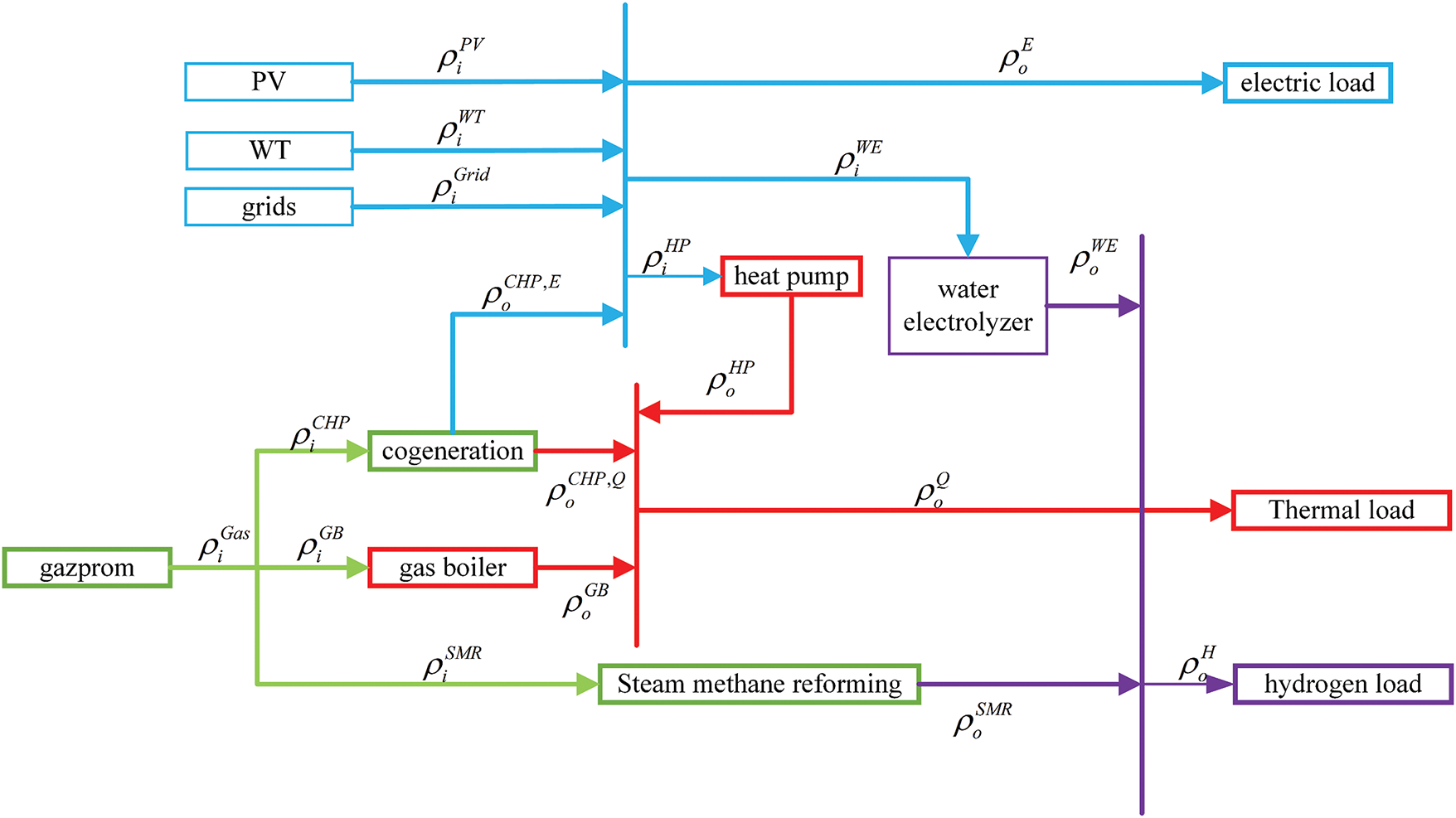
Figure 1: Schematic diagram of the structure of the EHH-IES based on carbon emission flow

In Fig. 1, ρiPV, ρiWT, ρiGrid, ρiGas are the carbon emission densities of the photovoltaic, wind, grid, and natural gas energy input ports, respectively. ρoE, ρoQ, ρoH are the carbon emission densities of the electricity, heat, and hydrogen output ports, respectively. ρiWE, ρiHP, ρiCHP, ρiGB, ρiSMR are the carbon emission densities at the inputs of water electrolyzer, heat pump, cogeneration, gas boiler, and steam methane reformer, respectively. ρoWE, ρoHP, ρoGB, ρoSMR are the carbon emission densities at the output of water electrolyzer, heat pump, gas boiler and methane reforming equipment, respectively. ρoCHP,E, ρoCHP,Q represent the carbon emission densities of the cogeneration equipment’s outputs to the electrical grid and the heating grids, respectively.

The energy flow in EHH-IES is transmitted from the input to the output end through many energy conversion devices. Due to the diversity of energy conversion devices, this paper constructs an energy coupling model to simplify the complex process of multiple energy input-conversion-output in EHH-IES into the relationship between the input and output ports, thus, for the ease of computing the carbon emission density for energy conversion within EHH-IES, it is represented in the model as follows:

ρoE=ρiPVPiPV+ρiWTPiWT+ρiGridPiGrid+ρoCHP,EPoCHP,EPiPV+PiWT+PiGrid+PoCHP,E(4)

where PiPV (kW) is the PV input power, PiWT (kW) is the wind input power, PiGrid (kW) is the grid input power, and PoCHP,E (kW) is the output power of the CHP used for power generation.

ρoQ=ρoCHP,QPoCHP,Q+ρoHPPoHP+ρoGBPoGBPoCHP,E+PoHP+PoGB(5)

where PoCHP,Q (kW) is the output power of CHP for heat production, PoHP (kW) is the output power of heat pumps, and PoGB (kW) is the output power of gas boilers.

ρoE=ρoSMRPoSMR+ρoWEPoWEPoSMR+PoWE(6)

where PoSMR (kW) is the output power of the methane reforming equipment and PoWE (kW) is the output power of the water electrolyzer.

In EHG-IES, energy conversion devices have different conversion efficiencies due to the differences in conversion methods and the process of energy transformation. Thus, it can be concluded that:

ρiGas=ρiGB=ρiCHP=ρiSMR(7)

ρoE=ρiWE=ρiHP(8)

{ρoWE=ρiWE/ωWEρoHP=ρiHP/ωHPρoSMR=ρiSMR/ωSMRρoGB=ρiGB/ωGB(9)

{ρoCHP,Q=ρiCHP/ωCHP,QρoCHP,E=ρiCHP/ωCHP,E(10)

where ωWE, ωHP, ωSMR, ωGB, ωCHP,Q, ωCHP,E are the energy conversion efficiencies of water electrolyzer, heat pump, methane reforming equipment, gas boiler, cogeneration for heat production, and cogeneration for power generation, respectively [27,28].

Utilizing the energy coupling model, it is feasible to allocate carbon responsibility according to the carbon emission flow theory, by suitably distributing the carbon emission density from each energy flow within the EHH-IES system.

Based on the carbon emission flow theory and with the help of the energy coupling model, the carbon emission density generated by each energy flow in the EHH-IES can be reasonably allocated, thereby realizing the accurate division of carbon responsibilities.

2.3 Application Innovations of Carbon Emission Flow Definitions

The application of the aforementioned carbon emission flow definitions (carbon emissions, carbon emission rate, branch carbon emission density, and node carbon potential) demonstrates two innovations in the EHH-IES. Firstly, a breakthrough in quantifying hydrogen energy carbon flow. To address the gap where existing carbon emission flow theories do not cover hydrogen energy, this paper calculates the carbon emission intensity of WE and SMR using the branch carbon emission density formula (Eq. (2)). WE relies on grid electricity input, so its branch carbon emission density equals the carbon emission density of the grid input (e.g., ρWE = ρgrid/ωWE in Eq. (9)). SMR depends on natural gas input, and its carbon emission density is calculated by combining the carbon emission density of natural gas with conversion efficiency (ρSMR = ρgas/ωSMR). This achieves, for the first time, accurate tracking of carbon flow in hydrogen production processes.

Secondly, coupled calculation of node carbon potential for multi-energy flows. At nodes of multi-output devices such as CHP units, the node carbon potential (Eq. (3)) needs to integrate the weighted sum of carbon emission rates from both electricity and heat outputs, rather than a simple accumulation used for single-energy nodes. For example, the carbon emission density of CHP’s power output (ρCHP,E) differs from that of its heat output (ρCHP,Q) due to differences in conversion efficiency. The node carbon potential must be calculated by weighting the energy proportions of the two, which solves the problem of the “one-size-fits-all” approach to carbon responsibility for coupled devices in traditional methods.

3  Calculation of Carbon Trading Costs

3.1 Initial Carbon Credits

In the EHH-IES, the main energy networks include the power grid, heat grid, and hydrogen grid, and the initial carbon credit allocation is mainly composed of these three networks:

CEHG−IES=CE+CQ+CH(11)

where CEHG−IES (kg), CE (kg), CQ (kg), CH (kg) are the total initial carbon credits of the EHH-IES, the EHG-IES power grid, the EHH-IES heat grid, and the EHH-IES hydrogen grid, respectively.

(1)   Grids:

CE=CPV+CWT+CGrid+CCHP,E(12)

{CPV=λe∑t=1TPPV(t)CWT=λe∑t=1TPWT(t)CGrid=λe∑t=1TPGrid(t)CCHP,E=λeωCHP,E∑t=1TPCHP,E(t)(13)

where CPV (kg), CWT (kg), CGrid (kg), CCHP,E (kg) are the initial carbon credits for PV power generation, wind power generation, and transmission of power generation by the power company, λe (kg/kW) is the carbon credit per unit of electric power, and PPV(t) (kW), PWT(t) (kW), PGrid(t) (kW), PCHP,E(t) (kW) represent the heat generation power of cogeneration, heat pump, and gas boiler in period t, respectively.

(2)   Heat grids:

CQ=CCHP,Q+CHP+CGB(14)

{CCHP,Q=λqωCHP,Q∑t=1TPCHP,Q(t)CHP=λq∑t=1TPHP(t)CGB=λq∑t=1TPGB(t)(15)

where CCHP,Q (kg), CHP (kg), CGB (kg) are the initial carbon credits for heat generated by hot co-generation, heat pump and gas boiler, respectively, λq (kg/kW) is the carbon credits per unit of thermal power, PCHP,Q(t) (kW), PHP(t) (kW), PGB(t) (kW) is the energy of heat produced through co-generation, heat pump and gas boiler in time period t, respectively.

(3)   Hydrogen grids:

CH=CSMR+CWE(16)

{CSMR=λh∑t=1TPSMR(t)CWE=λh∑t=1TPWE(t)(17)

where CSMR (kg), CWE (kg) are the initial carbon credits for hydrogen production from steam methane reforming and water electrolyzer, respectively, λh (kg/kW) is the carbon credits per unit of hydrogen power, and PSMR(t) (kW), PWE(t) (kW) represent the hydrogen production power of steam methane reforming and water electrolyzer in period t, respectively.

The innovation in calculating the initial carbon credits lies in taking the node carbon potential as the quantitative basis. As shown in Eqs. (24)–(29), in the power grid credits, the node carbon potential of wind power/photovoltaics is 0, and their credits are only related to their output (CPV = λe·PPV(t)). While the credits for CHP power generation needs to be combined with its node carbon potential (reflecting carbon emissions from gas consumption), that is, CCHP,E = λe·ωCHP,E·PCHP,E(t). This allocation method based on carbon flow characteristics is more accurate than the traditional “average allocation according to installed capacity”, avoiding excessive credits for high-emission equipment which would weaken the motivation for emission reduction.

3.2 Real Carbon Emissions Modeling

According to the accounting methods in the IPCC Guidelines for National Greenhouse Gas Inventories, the construction of the actual carbon emission model is associated with the actual output power of the power grid, heat grid, and hydrogen grid within the EHH-IES:

{CEHH−IES,a=CaE+CaQ+CaHCaE=∑t=1T(a1+b1(PPV(t)+PWT(t)+PGrid(t)+PCHP,E(t))+c1(PPV(t)+PWT(t)+PGrid(t)+PCHP,E(t))2)CaQ=∑t=1T(a2+b2(PCHP,Q(t)+PHP(t)+PGB(t))+c2(PCHP,Q(t)+PHP(t)+PGB(t))2)CaH=∑t=1T(a3+b3(PSMR(t)+PWE(t))+c3(PSMR(t)+PWE(t))2)(18)

where CEHG−IES,a (kg), CaE (kg), CaQ (kg), CaH (kg) are the actual carbon emissions from the EHH-IES, the grid, the heat grids and the hydrogen grids, respectively; a1, b1, c1, a2, b2, c2, and a3, b3, c3 are the carbon emission calculation parameters of the grids, the heat grids and the hydrogen grids, respectively.

As a result, the carbon emissions Ca (kg) in EHH-IES that participate in carbon trading are as follows [29,30]:

Ca=CEHH−IES,a−CEHH−IES(19)

This study assumes that the buying and selling prices in carbon trading remain consistent, meaning that the purchase price when there is a positive carbon emission rights gap is the same as the selling price when there is a negative surplus. This is intended to form a more effective incentive mechanism for emission reduction.

3.3 Stepped Carbon Emissions Trading Model

To respond to the “dual-carbon” strategy and further reduce carbon emissions in integrated energy systems, this paper proposes the adoption of a stepped carbon pricing mechanism in the pricing stage of carbon emission trading. An incremental stepped carbon price will be imposed on the part that exceeds the initial carbon credits to enhance the system’s motivation for emission reduction. There are temporal and spatial differences in the carbon emission density of branches (for example, the carbon emission density of gas-fired boiler branches during peak hours is higher than that during off-peak hours). Such differences affect the deviation degree between actual carbon emissions and initial carbon credits through Eq. (19), and then trigger different intervals of the stepped carbon pricing mechanism (Eq. (20)). Among them, the carbon emissions of branches with high carbon emission density will be prioritized to enter higher steps, enabling carbon price regulation to accurately target high-emission links, thus overcoming the limitation of the traditional single carbon price, which regulates the entire system in a “non-discriminatory” manner.

The stepped carbon price divides multiple trading intervals based on carbon credits, as shown in Fig. 2, and the model is as follows [12,20]:

STA={ζCa,Ca≤LζL+ζ(1+α)(Ca−L),L≤Ca≤2LζL(2+α)+ζ(1+2α)(Ca−2L),2L≤Ca≤3LζL(3+3α)+ζ(1+3α)(Ca−3L),3L≤Ca≤4LζL(4+6α)+ζ(1+4α)(Ca−4L),4L≤Ca≤5L(20)

where STA is the stepped carbon price (CNY), ζ is the base carbon price (CNY/kg), α is the stepwise growth rate of the basic carbon price, and L is the length of the step interval.

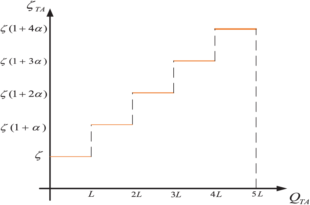
Figure 2: Tiered carbon price

4  Optimal Scheduling of EHH-IES Considering Carbon Emission Flow Theory and Wind-Solar Accommodation

4.1 Objective Function

This study, considering the economic efficiency of the EHH-IES and its capacity for integrating new energy, constructs an optimized objective function aiming at minimizing economic costs and the energy consumption of the integrated energy system.

minF=fs+fl(21)

where fs is the economic cost and fl is the energy loss.

fs=SE+SQ+SH+STA+SF(22)

{SE=DE∑t=1T(PPV(t)+PWT(t)+PGrid(t)+PCHP,E(t))SQ=DQ∑t=1T(PCHP,Q(t)+PHP(t)+PGB(t))SH=DH∑t=1T(PSMR(t)+PWE(t))SF=DPV∑t=1T(PPVF(t)−PPV(t))+DWT∑t=1T(PWTF(t)−PWT(t))(23)

where SE is the grid operating cost (CNY), SQ is the heat grids operating cost (CNY), SH is the hydrogen grids operating cost (CNY), and SF is the penalty cost for wind and light abandonment (CNY); DE (CNY/kW) is the unit grid operating cost, DQ (CNY/kW) is the unit thermal grids operating cost, and DH (CNY/kW) is the unit hydrogen grids operating cost; DPV and DWT are the unit penalty cost for solar abandonment and the unit penalty cost for wind abandonment, respectively; PPVF(t) (kW) and PWTF(t) (kW) are the predicted outputs of photovoltaic power generation and wind power generation, respectively.

fl=∑t=1T(LWE(t)+LHP(t)+LCHP(t)+LGB(t)+LSMR(t))(24)

{LWE(t)=PWE(t)(1−ωWE)LHP(t)=PHP(t)(1−ωHP)LCHP(t)=(PCHP.E(t)+PCHP.Q(t))(1−ωCHP.E−ωCHP.Q)LGB(t)=PGB(t)(1−ωGB)LSMR(t)=PSMR(t)(1−ωSMR)(25)

where LWE(t) (kW), LHP(t) (kW), LCHP(t) (kW), LGB(t) (kW), LSMR(t) (kW) are the energy losses of water electrolyzer, heat pump, cogeneration, gas boiler, and steam methane reforming, respectively. Since the carbon emission flow theory is based on energy flow for calculation, the carbon emission density conversion rate in the EHH-IES is consistent with the energy conversion rate [31,32].

For the multi-objective function, the weight selection is not fixed. Instead, it is dynamically adjusted based on the node carbon potential and branch carbon emission density in the carbon emission flow theory, and optimized in combination with the stepped carbon price mechanism and actual operational constraints. Specifically, for renewable energy sources such as wind and solar with zero carbon emission density, during their peak output periods, a higher weight is assigned to the penalty cost for wind-solar curtailment to prioritize the absorption of clean energy. The weight of carbon trading cost for high-emission equipment (such as gas boilers) increases with their carbon emission density, while the carbon cost weight for low-emission equipment (such as heat pumps) is relatively lower. This adjustment is automatically achieved through the nonlinear characteristics of the stepped carbon price (the carbon price increases by a 25% growth rate when exceeding the quota). In addition, the base weight of the operation cost is determined according to actual energy prices (e.g., grid electricity price, natural gas price), and the weight of wind-solar curtailment penalty (0.2 CNY/kWh) is set with reference to the industry’s economic loss coefficient for curtailment. Finally, the weights of each objective are implicitly optimized during the iteration process using the CPLEX solver, ensuring the optimal balance between economy and low carbon under the constraints of power balance and equipment operation.

4.2 Restrictive Condition

4.2.1 Power Balance Constraints

(1)   Electric power balance constraint

• Because of the uncertainty of wind power generation, this study excludes the case of EHH-IES feeding to the higher grid, which reduces the grid fluctuation and improves the system stability.

{PGrid(t)=PE,Lord(t)+PWE(t)+PHP(t)−PCHP,E(t)−PPV(t)−PWT(t)0≤PGrid(t)≤PGrid,max(t)(26)

where PE,Lord(t) (kW) is the power of electric load at the moment t, PGrid,max(t) (kW) is the maximum value of grid output at the moment t.

(2)   Heat power balance constraint

PCHP,Q(t)+PGB(t)+PHP(t)=PQ,Lord(t)(27)

where PQ,Lord(t) (kW) is the thermal load power at time t.

(3)   Hydrogen power balance constraint

PSMR(t)+PWE(t)=PH,Lord(t)(28)

where PH,Lord(t) (kW) is the hydrogen load power at time t.

4.2.2 Crew Constraints

(1)   Wind and light output constraints:

{PPVmin(t)≤PPV(t)≤PPVmax(t)PWTmin(t)≤PWT(t)≤PWTmax(t)(29)

where PPVmin(t) (kW) and PPVmax(t) (kW) are the minimum and maximum outputs of photovoltaic power generation at time t; PWTmin(t) (kW) and PWTmax(t) (kW) are the minimum and maximum outputs of wind power generation at time t.

(2)   Cogeneration output and creep constraints:

{ωCHP,EPCHPmin(t)≤PCHP,E(t)≤ωCHP,EPCHPmax(t)ωCHP,QPCHPmin(t)≤PCHP,Q(t)≤ωCHP,QPCHPmax(t)−φCHPdownωCHP,EΔt≤PCHP,E(t)−PCHP,E(t−1)≤φCHPupωCHP,EΔt−φCHPdownωCHP,QΔt≤PCHP,Q(t)−PCHP,Q(t−1)≤φCHPupωCHP,QΔt0≤ωCHP,E+ωCHP,Q≤1(30)

where PCHPmin(t) (kW) and PCHPmax(t) (kW) are the minimum and maximum output of cogeneration at time t, −φCHPdown (kW/h) and φCHPup (kW/h) are the upper and lower limits of heat pump climbing power, Δt (h) is a scheduling cycle.

(3)   EHH-IES operation equipment constraints:

{PGBmin(t)≤PGB(t)≤PGBmax(t)PHPmin(t)≤PHP(t)≤PHPmax(t)PSMRmin(t)≤PSMR(t)≤PSMRmax(t)PWEmin(t)≤PWE(t)≤PWEmax(t)(31)

In the formula, PGBmin(t) (kW) and PGBmAX(t) (kW) are the minimum and maximum heat output of the gas boiler at time t, PHPmin(t) (kW) and PHPmAX(t) (kW) are the minimum and maximum heat output of the heat pump at time t, and the minimum and maximum steam methane reforming output at time t, PWEmin(t) (kW) and PWEmax(t) (kW) are the minimum and maximum hydrogen production output of the water electrolyzer at time t, respectively.

4.2.3 Contact Line Yransmission Power Constraints

PLinemin(t)≤PLine(t)≤PLinemax(t)(32)

where PLine(t) (kW), PLinemin(t) (kW), PLinemax(t) (kW) are the grid contact line transmission power, grid contact line transmission minimum and maximum power at time t, respectively.

4.2.4 Natural Gas Grid Constraints

The primary objective of the natural gas grids is to ensure a steady supply of natural gas both to the heating grids and to the hydrogen grids, considering factors such as the gas source, nodal pressure levels, and the constraints of natural gas pipeline flows:

{Vamin≤Va,t≤Vamaxpimin≤pi≤pimaxQij,t=χijsgn(pi,t−pj,t)|pi,t2−pj,t2|sgn(pi,t−pj,t)={1,pi,t≥pj,t−1,pi,t≤pj,t(33)

where Va,t (m3) is the gas supply from gas source a at time t, Vamin (m3) and Vamax (m3) is the minimum and maximum value of gas supply from gas source a; pi (pa) is the pressure at node i, pimin (pa) and pimax (pa) is the lower and upper limit of the pressure that node i can withstand; Qij,t (m3/h) is the natural gas flow rate between node i and node j at time t, χij is the natural gas pipeline transmission parameter, sgn(pi,t−pj,t) is the natural gas transmission direction parameter [33,34].

4.3 Constraint Model Solving

The model solution process is as follows, which is shown in Fig. 3:

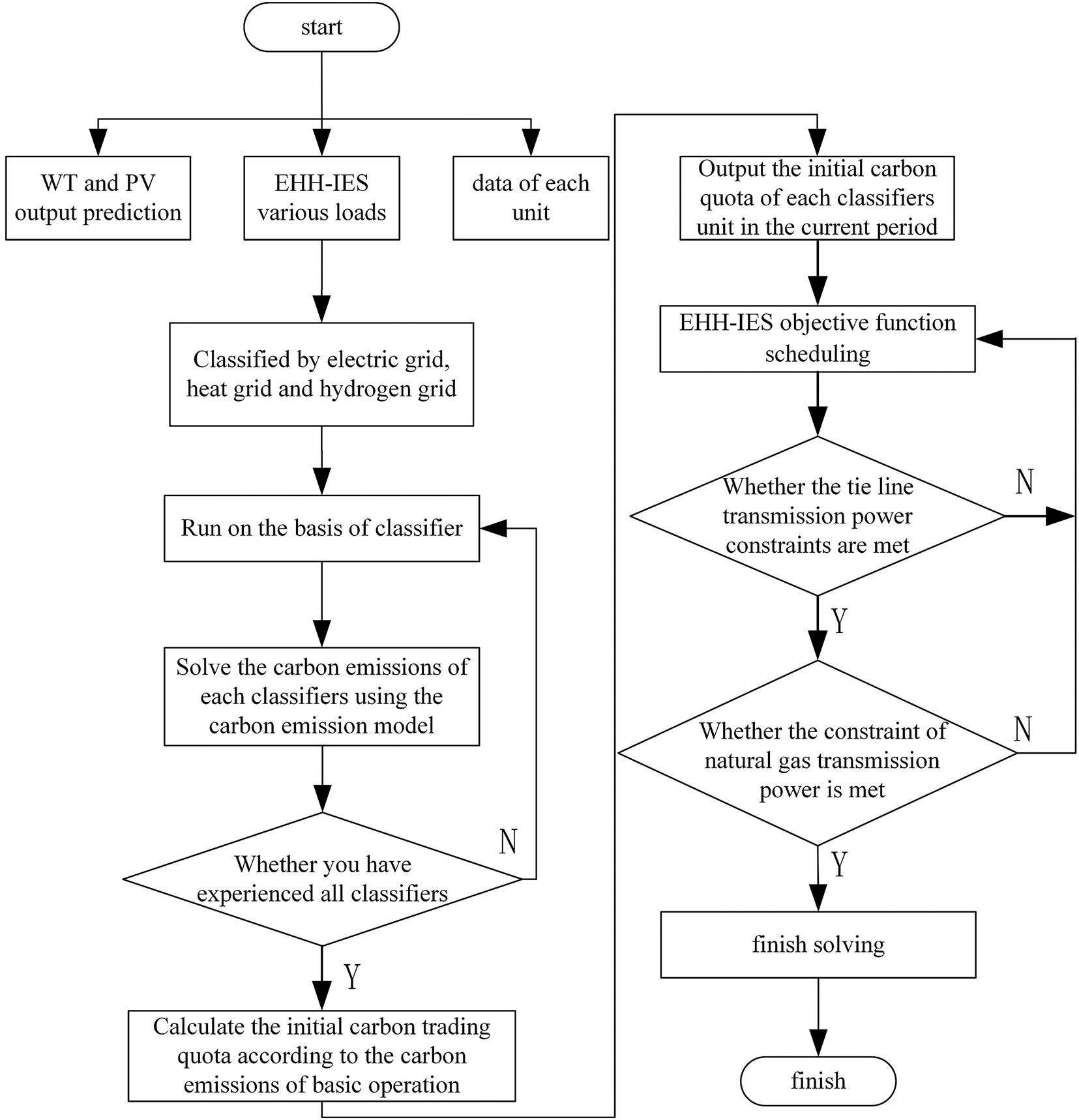
Figure 3: Solution flowchart

1.    Initialize the predicted output of wind and solar, various types of loads, unit parameters, and line-node parameters.

2.    Make the power grid, natural gas grid, and hydrogen grid operate initially, and calculate the initial carbon emission allowances for each network in the EHH-IES.

3.    Dispatch each energy conversion device in the EHH-IES, and calculate the tie-line power and natural gas transmission volume in the system network.

4.    If the line constraints of the power grid and natural gas grid are satisfied, output the dispatch result; if not, return to step 3 and re-perform the dispatch calculation.

5.    Output and analyze the dispatch result.

4.4 Model Solution Method and Process

The optimal scheduling model for the EHH-IES considering carbon emission flow and wind-solar accommodation constructed in this paper is a Mixed Integer Linear Programming (MILP) model, which includes multi-objective functions (minimization of operation cost, carbon trading cost, wind-solar accommodation penalty cost, and energy loss) and nonlinear constraints (such as stepped carbon pricing mechanism, multi-energy flow coupling constraints, etc.). In view of the complexity and constraint characteristics of the model, the Yalmip modeling tool and CPLEX solver are used jointly for solution, and the specific methods are as follows.

(1)  Model transformation: Nonlinear constraints are transformed into linear forms through linearization processing. For example, for the piecewise function of the stepped carbon pricing mechanism (Eq. (20)) in Section 3.3, binary variables are introduced to identify the stepped interval where carbon emissions are located, so as to convert the nonlinear carbon trading cost into a linear expression; for the thermoelectric coupling constraint (Eq. (10)) of Combined Heat and Power (CHP), the nonlinear conversion relationship is linearized through efficiency coefficients to ensure that the model meets the requirements of MILP solution.

(2)  Solver configuration: The CPLEX solver is used to handle the transformed linear programming problem. As a commercial optimization solver, CPLEX has the ability to efficiently handle large-scale integer programming and linear constraints, and can quickly find the optimal solution under a given convergence accuracy (set to 1e−6 in this paper), which is suitable for solving the optimal problem of integrated energy systems involving multi-energy coupling and multi-period scheduling.

(3)  Solution process:

1.    Initialize parameters: Input the predicted output of wind and solar, electricity/heat/hydrogen load data, equipment parameters (capacity, conversion efficiency, climbing constraints, etc.) and carbon trading parameters (basic carbon price, stepped interval length, growth rate, etc.). Construct constraint matrix: Transform the power balance constraints, equipment operation constraints, tie-line transmission constraints, etc., in Section 4.2 into matrix forms, and form a complete optimization model together with the objective function;

2.    Iterative optimization: Perform global optimization on the 24-h scheduling cycle (with 1 h as the step size) through the CPLEX solver, and output the optimal decision variables such as equipment output, purchased electricity, and carbon emissions in each period;

3.    Constraint verification: If the solution results meet all constraint conditions (such as power balance error ≤ 1e−3 kW, carbon emission calculation deviation ≤ 1e−2 kg), output the final scheduling scheme; otherwise, return to the parameter adjustment stage, re-optimize the equipment operation boundary conditions and solve again [35].

Through the above methods, the model can be solved efficiently and the global optimal solution can be obtained, ensuring that the scheduling scheme meets the objectives of economy, low carbon and wind-solar accommodation, while conforming to the physical constraints of system operation.

5  Simulation Results Analysis

5.1 Basic Data

To verify the effectiveness of the proposed scheduling method, this paper constructs a case of an IES including electricity-heat-hydrogen coupling equipment. The specific parameters and data selection are as follows.

5.1.1 Load and Wind-Solar Output Data

The daily variation curves of electricity, heat, hydrogen loads and predicted wind-solar outputs are shown in Fig. 4. The data are generated based on the statistical analysis of the actual energy consumption characteristics of a typical mixed park of residents and commerce [28]. Among them, the peak value of the electricity load appears at 18:00 (3200 kW), and the valley value appears at 4:00 (1500 kW); the heat load, due to heating demand, has a peak value at 10:00 (1800 kW); the hydrogen load is mainly used for the standby power supply of fuel cells and remains relatively stable throughout the day (about 500 kW). The peak value of the photovoltaic output appears at 12:00 (1800 kW), which is in line with the characteristics of typical sunny-day illumination; the wind power output has two peak values at 3:00 in the early morning and 22:00 at night (1200 and 1000 kW, respectively) [36].

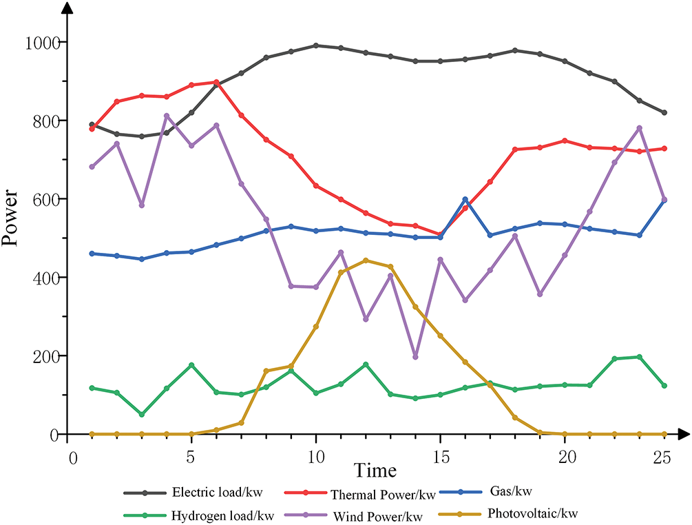
Figure 4: Forecast load

5.1.2 Equipment Parameters

The installed capacity, conversion efficiency, and climbing constraint parameters of each energy conversion device in the EHH-IES are shown in Table 1, with the parameter selection basis as follows.

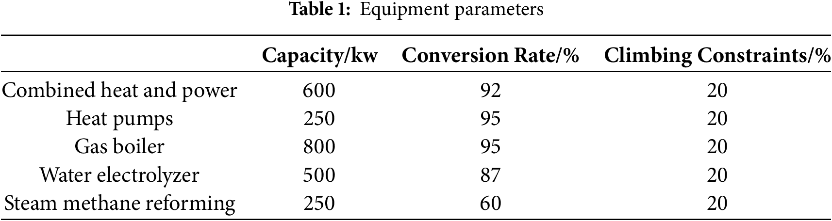
The CHP unit has a capacity of 600 kW and a total thermoelectric conversion efficiency of 92%, referring to the efficiency characteristics of the combined operation of gas turbines and waste heat boilers. Its Climbing constraints is limited to 20%, which conforms to the operation specifications for small and medium-sized distributed CHP. The HP has a capacity of 250 kW and a heating efficiency of 95%, based on the typical performance of air-source heat pumps in an environment of −5~15°C. The GB has a capacity of 800 kW and an efficiency of 95%, referring to the design parameters of industrial-grade natural gas boilers. The WE has a capacity of 500 kW and an electrolysis efficiency of 87%, adopting the typical efficiency curve of alkaline electrolyzers. The SMR has a capacity of 250 kW and a hydrogen production efficiency of 60%, considering the energy loss in methane reforming and water-gas shift reactions [37].

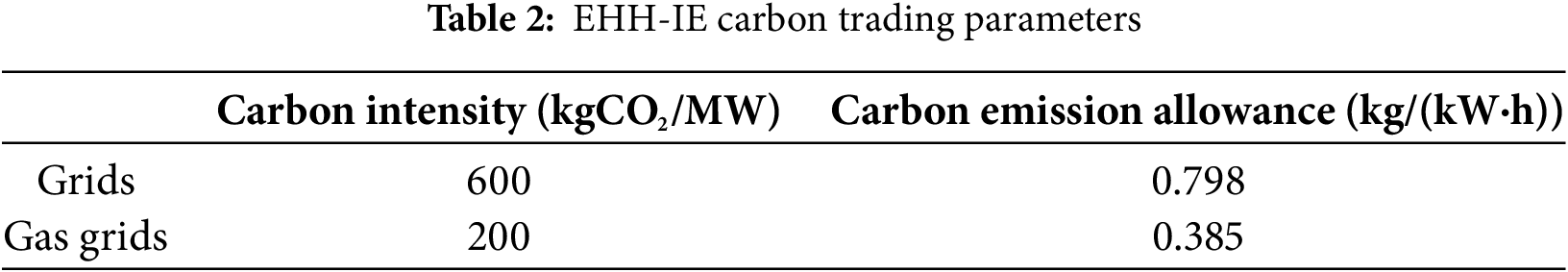
5.1.3 Carbon Trading and Penalty Cost Parameters

Parameters related to carbon trading are shown in Table 2. Among them, the carbon emission intensity of the power grid is set at 600 kgCO2/MWh, corresponding to the average emission level of regional thermal power units. The carbon emission intensity of the natural gas grid is 200 kgCO2/MWh, referring to the emission factor for natural gas combustion specified by the IPCC. The carbon credit is 0.798 kg/(kW·h) for the power grid and 0.385 kg/(kW·h) for the natural gas grid, which are based on the regional “carbon credit baseline” policy [38,39].

Other key parameters are set as follows. The unit penalty cost for curtailed wind and solar power is 0.2 CNY/(kW·h), with reference to the calculation of economic losses caused by the curtailment of renewable energy in. In the stepped carbon pricing mechanism, the interval length L is 2 t, the basic carbon price ζ is 250 yuan/t, and the growth rate α is 25%. These parameter settings refer to the gradient design of stepped carbon prices in, aiming to balance emission reduction incentives and economic feasibility [40,41].

5.1.4 Solution Parameters

The scheduling cycle is 24 h with a time step of 1 h. The model is built using the Yalmip toolbox, and the CPLEX 12.9 solver is called for solution, with the convergence accuracy set to 1 × 10−6. To compare the impact of different mechanisms on scheduling effects, three scheduling schemes are set as follows:

Scheme 1: Low-carbon economic scheduling of EHH-IES considering carbon trading (including the stepped carbon pricing mechanism) and penalty for curtailed wind and solar power. The objective function includes operation cost, carbon trading cost, penalty cost for wind-solar accommodation, and energy loss (Eqs. (21)–(25)).

Scheme 2: Scheduling of EHH-IES considering carbon trading (including the stepped carbon pricing mechanism) but without the penalty for curtailed wind and solar power. The wind-solar accommodation penalty term SF is removed from the objective function.

Scheme 3: Economic scheduling of EHH-IES without considering carbon trading or penalty for curtailed wind and solar power. The objective function only retains the operation cost and energy loss, i.e., min F = fs′ + fl (where fs′ = SE + SQ + SH).

5.2 Analysis of Results

Based on the simulation results of the three scheduling schemes, this section conducts an analysis from three aspects: the collaborative optimization of cost and carbon emissions, the inherent logic of multi-energy flow power balance, and the mechanism of improving wind-solar accommodation. It reveals how the proposed model achieves the collaborative goal of “low carbon-economy-high accommodation” through carbon emission flow tracking and the stepped carbon pricing mechanism.

5.2.1 Collaborative Optimization of Cost and Carbon Emissions

Figs. 5–7 appearing in this section correspond to option 1, option 2, and option 3, respectively.

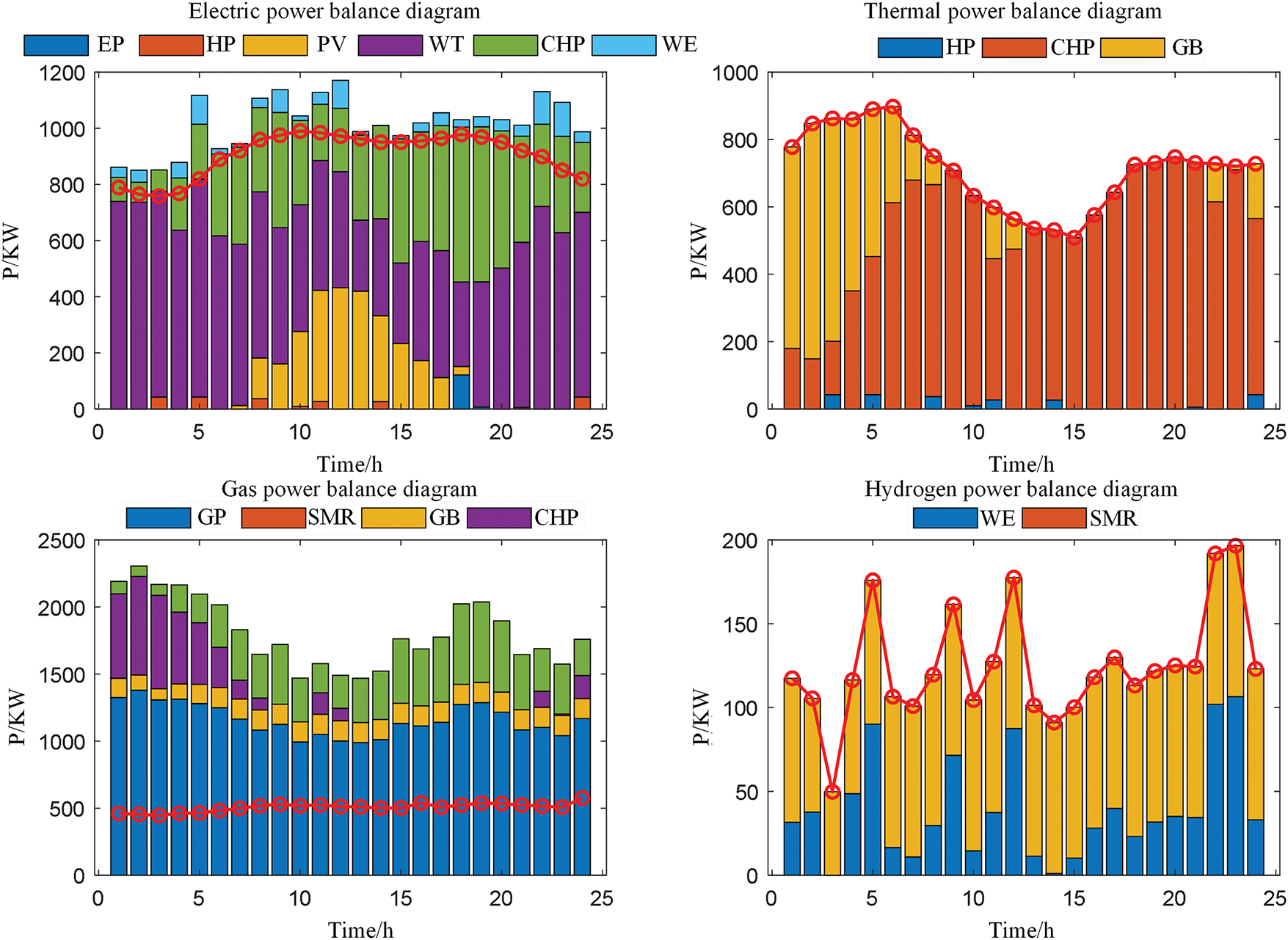
Figure 5: Option 1 system master dispatch diagram

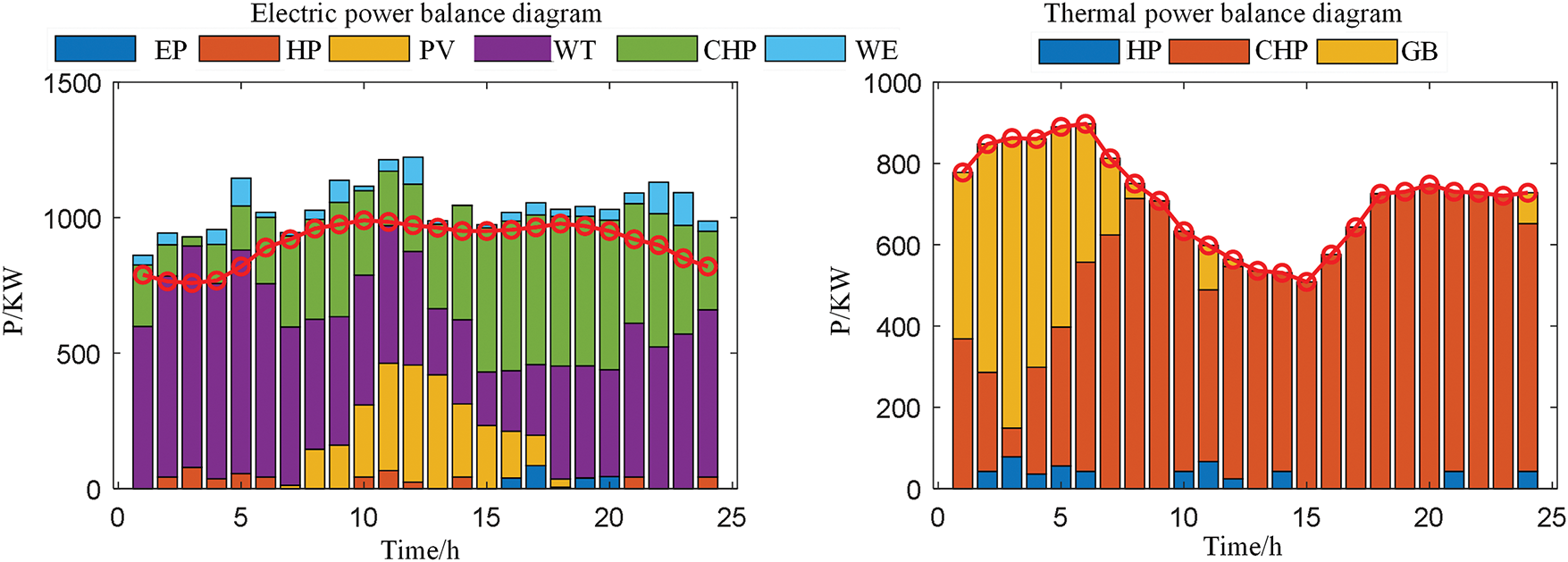
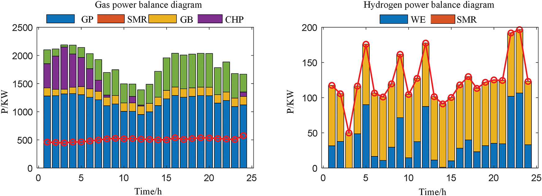
Figure 6: Option 2 system master dispatch diagram

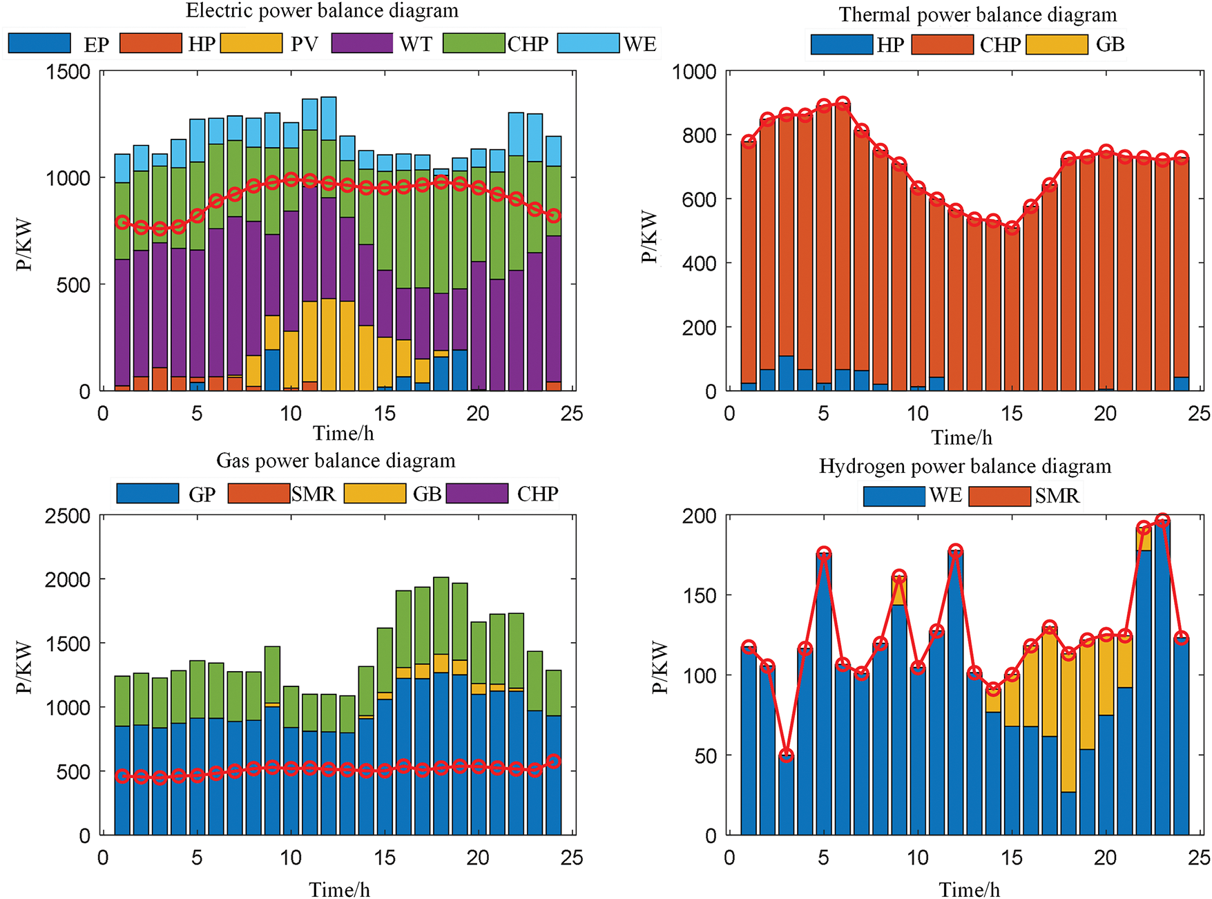
Figure 7: Option 3 system master dispatch diagram

Data in Table 3 shows that, compared with Scheme 3 (pure economic dispatch), Scheme 1 (considering carbon trading and wind-solar accommodation penalties) leads to an increase in total cost by 16.10%, while reducing carbon emissions by 53.97% and the amount of curtailed wind and solar power by 68.89%. This result directly confirms the effectiveness of the core model in this paper. Through the collaborative mechanism of “accurate measurement of carbon emission flow, stepped carbon price incentives, and wind-solar accommodation constraints”, the goal of “achieving deep emission reduction and high accommodation with a small increase in cost” has been realized.

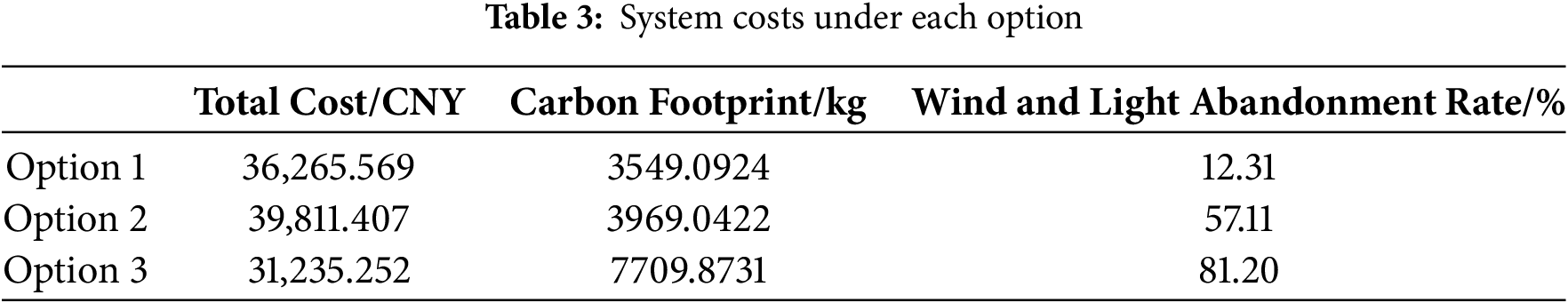
The reasons are analyzed from the mechanism level as follows. Since Scheme 3 does not consider carbon trading and wind-solar accommodation penalties, its dispatch logic is completely oriented to “minimum operating cost”, resulting in heavy reliance on grid power purchase with high carbon emissions (Fig. 7 shows that its peak power purchase reaches 2200 kW) and gas-fired boiler heating, with carbon emissions as high as 7709.87 kg; meanwhile, due to the absence of penalties for wind-solar curtailment, surplus wind and solar output is directly curtailed (the curtailment rate of wind and solar power reaches 81.20%), which not only wastes clean energy but also intensifies dependence on traditional energy sources.

After introducing carbon trading in Scheme 2, the stepped carbon price imposes constraints on high-carbon emission behaviors (e.g., the carbon cost surges when the output of gas-fired boilers exceeds the threshold), reducing carbon emissions to 3969.04 kg (a 48.51% decrease compared with Scheme 3). However, due to the lack of wind-solar accommodation penalties, the system still tends to curtail wind and solar output with large fluctuations (the curtailment rate of wind and solar power is 57.11%), leading to still high power purchase (peak power purchase of 1800 kW in Fig. 6), and the total cost is 8.91% higher than that of Scheme 1 (because the power purchase cost is not replaced by wind and solar energy).

Scheme 1, through the wind-solar accommodation penalty, forces the system to give priority to accommodating wind and solar output (Fig. 5 shows that photovoltaic and wind power outputs are fully utilized for 18 h), reducing grid power purchase (peak power purchase drops to 800 kW), which not only reduces carbon emissions from traditional thermal power but also lowers power purchase costs; at the same time, the stepped carbon price accurately increases prices for high-carbon emission links (such as the output of gas-fired boilers at 18:00), forcing the system to adopt more low-carbon CHP heating (the proportion of CHP heating increases to 60%), ultimately achieving a significant double reduction in carbon emissions and the amount of curtailed wind and solar power.

5.2.2 Inherent Logic of Multi-Energy Flow Power Balance: Guiding Role of Carbon Emission Flow

The differences in power balance among the three schemes (Figs. 5–7) essentially lie in the logical divergence between “low-carbon priority dispatch based on carbon emission flow tracking” and “pure economic dispatch”, which is specifically reflected in the coupling optimization of the electricity, heat, and hydrogen networks.

Electricity network balance: In Scheme 1, the carbon emission flow theory is used to identify the “zero carbon emission density” characteristic of photovoltaic and wind power (with branch carbon emission density ρBCI = 0), so they are prioritized in power balance (as shown in Fig. 5, the 1800 kW photovoltaic output from 10:00 to 15:00 is fully absorbed). Grid power purchase is only supplemented when wind and solar power are insufficient (e.g., 500 kW purchased at 4:00 a.m.). However, Scheme 3 ignores the differences in carbon emission density and still purchases electricity when wind and solar power are abundant (e.g., 1200 kW purchased at 12:00), leading to a surge in carbon emissions. This confirms the guiding role of the carbon emission flow theory in “prioritizing the absorption of low-carbon energy”. By quantifying the carbon emission density of different power sources, it provides a clear low-carbon priority for power balance.

Heat network balance: In Scheme 1, the heat load is mainly met by CHP units (accounting for 60%), and gas-fired boilers only supplement energy when the CHP output is insufficient (e.g., 300 kW output at 20:00). This is because carbon emission flow calculations show that the carbon emission density of the CHP heating branch (ρBCI,CHP,Q = 0.12 kg/kWh) is lower than that of gas-fired boilers (ρBCI,GB = 0.25 kg/kWh). The stepped carbon pricing further amplifies this difference (the carbon price for gas-fired boilers’ over-quota emissions reaches 312.5 CNY/t), prompting the system to prioritize low-carbon heating paths. In Scheme 3, without carbon constraints, the output proportion of gas-fired boilers reaches 70% (Fig. 7), resulting in persistently high carbon emissions in the heat network.

Hydrogen network balance: In Scheme 1, the hydrogen load is mainly met by hydrogen production from WE (accounting for 70%), with SMR only as a supplement (30%). The reason is that WE relies on zero-carbon electricity from photovoltaics/wind power (node carbon potential ρNCI,WE = 0), while SMR depends on natural gas (ρNCI,SMR = 0.20 kg/kWh). Carbon emission flow tracking accurately quantifies the low-carbon advantage of WE. Combined with carbon trading costs, the comprehensive cost of hydrogen production by WE is lower than that by SMR (0.3 CNY/kWh vs. 0.5 yuan/kWh). In Schemes 2 and 3, due to the lack of carbon flow guidance or absorption constraints, the proportion of hydrogen production by SMR reaches over 60%, pushing up carbon emissions in the hydrogen network.

5.2.3 Mechanism for Improving Wind-Solar Accommodation: Synergy between Penalty Constraints and Multi-Energy Complementarity

As shown in Fig. 8, the wind-solar curtailment rate of Scheme 1 (12.31%) is significantly lower than that of Scheme 2 (57.11%) and Scheme 3 (81.20%). The core lies in the synergy between wind-solar accommodation penalties and multi-energy flow complementarity, and this process relies on the accurate characterization of “the energy value of wind and solar” by the carbon emission flow theory.

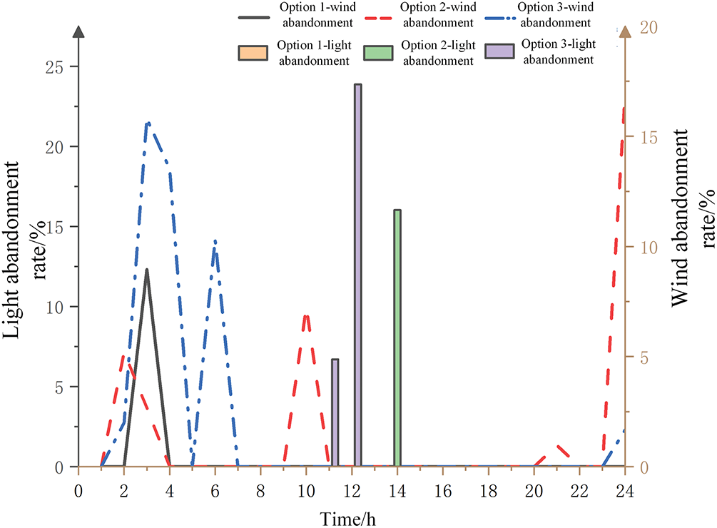
Figure 8: Wind and light abandonment rate

From a time dimension, during the peak photovoltaic output period (10:00–15:00), Scheme 1 absorbs surplus electric energy through the following paths.

Driving the WE to operate at full capacity (500 kW), converting electric energy into hydrogen for storage (the hydrogen network load is only 500 kW, and surplus hydrogen can be temporarily stored).

Increasing the output of the HP to 250 kW, enhancing heating reserves (the heat network load is 1200 kW, and surplus heat is temporarily stored through heat storage devices).

In this process, the carbon emission flow theory quantifies the carbon emission reduction benefits of converting “photovoltaic electric energy to hydrogen/heat energy” (each kWh of photovoltaic electricity absorbed reduces 0.6 kgCO2 emissions from grid power purchase). Meanwhile, the wind-solar accommodation penalty (0.2 CNY/kWh) economically forces the system to tap into such conversion potential.

In contrast, for Schemes 2 and 3: Scheme 2, without penalty constraints, directly curtails photovoltaic output when it exceeds the electric load (e.g., 11.65% of photovoltaic power is curtailed at 12:00); Scheme 3 not only curtails wind and solar power but also actively reduces CHP power generation due to low power purchase costs (the CHP electric power output is only 200 kW in Fig. 7), further narrowing the accommodation space for wind and solar energy. This indicates that the wind-solar accommodation penalty is a key constraint for “releasing multi-energy complementarity potential”, while the carbon emission flow theory provides a quantitative basis for “which complementary paths are more low-carbon”. The combination of the two realizes a significant improvement in the wind-solar accommodation rate.

In summary, the simulation results verify the core argument of this paper from three aspects: cost synergy, multi-energy flow balance, and wind-solar accommodation. Accurate carbon tracking based on carbon emission flow provides “navigation” for low-carbon dispatching, while the stepped carbon price and wind-solar accommodation penalty form a dual driving force of “economic incentives + constraints”, ultimately achieving the collaborative optimization of “low carbon-economy-high accommodation” for the EHH-IES.

6  Conclusions

This paper constructs a low-carbon economic dispatch model for the EHH-IES considering carbon emission flow and wind-solar accommodation. The core idea is as follows: the carbon emission flow model is used to accurately calculate the carbon emissions of the system and each energy conversion device. On this basis, the initial carbon quota is reasonably allocated, and combined with the characteristics of wind-solar accommodation, optimal dispatch is realized under the premise of balancing economy and low carbon.

Combined with the case analysis, the following conclusions are drawn. First, compared with traditional carbon metering methods, the carbon emission flow calculation model can more accurately quantify the carbon emissions of each energy network and conversion device in the integrated energy system, providing a reliable basis for carbon responsibility division and initial carbon quota allocation. Second, the carbon trading model introducing stepped carbon prices can strengthen the carbon emission constraints of each energy network and effectively guide the system to reduce carbon emissions. Third, adding a wind-solar accommodation penalty mechanism to the carbon trading model can not only further reduce carbon emissions but also optimize the system operation cost, balance the operation status of each energy conversion device, and realize the coordinated dispatch of economy and low carbon.

From the perspective of the innovative value of carbon theory application, the breakthroughs of this paper are reflected in three aspects: first, extending the carbon emission flow theory to the electricity-heat-hydrogen system, filling the gap in the quantification of hydrogen energy carbon flow; second, constructing a linkage mechanism between initial quotas based on node carbon potential and stepped carbon prices, solving the problem of “coarsening” regulation of traditional carbon trading on multi-energy flow systems; third, through the combination of carbon flow quantification and wind-solar accommodation penalties, enabling emission reduction measures to accurately target high-emission links and low-accommodation scenarios. The simulation results verify the effectiveness of these innovations. Compared with traditional methods, the model can reduce carbon emissions by 53.97% and curtailment of wind and solar power by 68.89%.

Future research can be deepened in three aspects. Firstly, optimizing the stepped carbon price into a dynamic penalty mechanism to improve the flexibility of the carbon trading mechanism. Secondly, constructing a coupled dispatch model of power purchase, gas purchase and carbon price to enhance the multi-energy collaborative optimization capability. Thirdly, exploring the day-ahead and intraday joint dispatch mode to further improve the engineering applicability of the model.

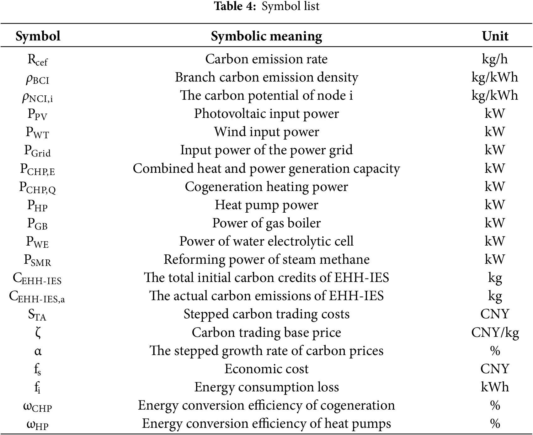
The following Table 4 expresses the units of physical quantities in this paper.

Acknowledgement: Not applicable.

Funding Statement: The authors received no specific funding for this study.

Author Contributions: The authors confirm contribution to the paper as follows: Study conception and design: Yukun Yang, Jun He; Data collection: Kun Chen; Analysis and interpretation of results: Yukun Yang; Draft manuscript preparation: Zhi Li, Wenfeng Chen. All authors reviewed the results and approved the final version of the manuscript.

Availability of Data and Materials: The raw data supporting the conclusion of this article will be made available by the authors with reasonable request.

Ethics Approval: Not applicable.

Conflicts of Interest: The authors declare no conflicts of interest to report regarding the present study.

References

1. Tang BJ, Cao XL, Li R, Xiang ZB, Zhang S. Economic and low-carbon planning for interconnected integrated energy systems considering emerging technologies and future development trends. Energy. 2024;302:131850. doi:10.1016/j.energy.2024.131850. [Google Scholar] [CrossRef]

2. Qin C, Yan Q, He G. Integrated energy systems planning with electricity, heat and gas using particle swarm optimization. Energy. 2019;188:116044. doi:10.1016/j.energy.2019.116044. [Google Scholar] [CrossRef]

3. Ma T, Wu J, Hao L. Energy flow modeling and optimal operation analysis of the micro energy grid based on energy hub. Energy Convers Manage. 2017;133:292–306. doi:10.1016/j.enconman.2016.12.011. [Google Scholar] [CrossRef]

4. Gong Y, Yang X, Xu J, Chen C, Zhao T, Liu S, et al. Optimal operation of integrated energy system considering virtual heating energy storage. Energy Rep. 2021;7:419–25. doi:10.1016/j.egyr.2021.01.051. [Google Scholar] [CrossRef]

5. Zhang Z, Wang C, Yang M, Chen X, Lv H. Day-ahead optimal dispatch for integrated energy system considering power-to-gas and dynamic pipeline networks. In: 2020 IEEE Industry Applications Society Annual Meeting; 2020 Oct 10–16; Detroit, MI, USA. p. 1–7. doi:10.1109/ias44978.2020.9334831. [Google Scholar] [CrossRef]

6. Wu C, Gu W, Xu Y, Jiang P, Lu S, Zhao B. Bi-level optimization model for integrated energy system considering the thermal comfort of heat customers. Appl Energy. 2018;232:607–16. doi:10.1016/j.ijepes.2023.109168. [Google Scholar] [CrossRef]

7. Wang L, Dong H, Lin J, Zeng M. Multi-objective optimal scheduling model with IGDT method of integrated energy system considering ladder-type carbon trading mechanism. Int J Electr Power Energy Syst. 2022;143:108386. doi:10.1016/j.ijepes.2022.108386. [Google Scholar] [CrossRef]

8. Guo Z, Zhang R, Wang L, Zeng S, Li Y. Optimal operation of regional integrated energy system considering demand response. Appl Therm Eng. 2021;191:116860. doi:10.1016/j.applthermaleng.2021.116860. [Google Scholar] [CrossRef]

9. Han X, Ren J, Zhan L, Yang J, Huang P. Research on optimization of multi-energy coupling source-network-load-storage based on micro energy network. J Phys Conf Ser. 2024;2728(1):012069. doi:10.1088/1742-6596/2728/1/012069. [Google Scholar] [CrossRef]

10. Liu T, Yang Z, Duan Y, Hu S. Techno-economic assessment of hydrogen integrated into electrical/thermal energy storage in PV+ wind system devoting to high reliability. Energy Convers Manage. 2022;268:116067. doi:10.1016/j.enconman.2022.116067. [Google Scholar] [CrossRef]

11. Chen F, Liang H, Gao Y, Yang Y, Chen Y. Research on double-layer optimal scheduling model of integrated energy park based on non-cooperative game. Energies. 2019;12(16):3164. doi:10.3390/en12163164. [Google Scholar] [CrossRef]

12. Guo R, Ye H, Zhao Y. Low carbon dispatch of electricity-gas-thermal-storage integrated energy system based on stepped carbon trading. Energy Rep. 2022;8:449–55. doi:10.1016/j.egyr.2022.09.198. [Google Scholar] [CrossRef]

13. He L, Lu Z, Geng L, Zhang J, Li X, Guo X. Environmental economic dispatch of integrated regional energy system considering integrated demand response. Int J Electr Power Energy Syst. 2020;116:105525. doi:10.1016/j.ijepes.2019.105525. [Google Scholar] [CrossRef]

14. Fu B, Wang S, Quan Y. Low-carbon economic dispatch of an integrated energy system considering integrated demand response and ladder-type carbon trading mechanism. Amsterdam, The Netherlands: Elsevier B.V.; 2023. doi:10.2139/ssrn.4371941. [Google Scholar] [CrossRef]

15. Lu Q, Guo Q, Zeng W. Optimization scheduling of an integrated energy service system in community under the carbon trading mechanism: a model with reward-penalty and user satisfaction. J Clean Prod. 2021;323:129171. doi:10.1016/j.jclepro.2021.129171. [Google Scholar] [CrossRef]

16. Xiang Y, Guo Y, Wu G, Liu J, Sun W, Lei Y, et al. Low-carbon economic planning of integrated electricity-gas energy systems. Energy. 2022;249:123755. doi:10.1016/j.energy.2022.123755. [Google Scholar] [CrossRef]

17. Wang R, Cheng S, Zuo X, Liu Y. Optimal management of multi stakeholder integrated energy system considering dual incentive demand response and carbon trading mechanism. Int J Energy Res. 2021;46(5):6246–63. doi:10.1002/er.7561. [Google Scholar] [CrossRef]

18. Dai X. Low-carbon optimal dispatch of integrated energy systems taking into account the ladder-type carbon trading mechanism and electricity-heat demand response [Internet]. Berlin/Heidelberg, Germany: Springer Science and Business Media LLC.; 2024. doi:10.21203/rs.3.rs-4782796/v1. [Google Scholar] [CrossRef]

19. Zhang Y, Liu Z, Wu Y, Li L. Research on optimal operation of regional integrated energy systems in view of demand response and improved carbon trading. Appl Sci. 2023;13(11):6561. doi:10.3390/app13116561. [Google Scholar] [CrossRef]

20. Wang R, Wen X, Wang X, Fu Y, Zhang Y. Low carbon optimal operation of integrated energy system based on carbon capture technology, LCA carbon emissions and ladder-type carbon trading. Appl Energy. 2022;311:118664. doi:10.1016/j.apenergy.2022.118664. [Google Scholar] [CrossRef]

21. Tao H, Al Mamun K, Ali A, Solomin E, Zhou J, Sinaga N. Performance enhancement of integrated energy system using a PEM fuel cell and thermoelectric generator. Int J Hydrogen Energy. 2024;51:1280–92. doi:10.1016/j.ijhydene.2023.03.442. [Google Scholar] [CrossRef]

22. Li J, He X, Li W, Zhang M, Wu J. Low-carbon optimal learning scheduling of the power system based on carbon capture system and carbon emission flow theory. Electr Power Syst Res. 2023;218:109215. doi:10.1016/j.epsr.2023.109215. [Google Scholar] [CrossRef]

23. Cheng Y, Zhang N, Wang Y, Yang J, Kang C, Xia Q. Modeling carbon emission flow in multiple energy systems. IEEE Trans Smart Grid. 2019;10(4):3562–74. doi:10.1109/TSG.2018.2830775. [Google Scholar] [CrossRef]

24. Kang C, Zhou T, Chen Q, Xu Q, Xia Q, Ji Z. Carbon emission flow in networks. Sci Rep. 2012;2(1):479. doi:10.1038/srep00479. [Google Scholar] [PubMed] [CrossRef]

25. Li L, Yan F. How does density impact carbon emission intensity: insights from the block scale and an optimal parameters-based geographical detector. Land. 2024;13(7):1036. doi:10.3390/land13071036. [Google Scholar] [CrossRef]

26. Du R, Zhang M, Zhang N, Liu Y, Dong G, Tian L, et al. Evaluation of key node groups of embodied carbon emission transfer network in China based on complex network control theory. J Clean Prod. 2024;448:141605. doi:10.1016/j.jclepro.2024.141605. [Google Scholar] [CrossRef]

27. Zhang Y, Li J, Ji X, Ye P, Yu D, Zhang B. Optimal dispatching of electric-heat-hydrogen integrated energy system based on Stackelberg game. Energy Convers Econ. 2023;4(4):267–75. doi:10.1049/enc2.12094. [Google Scholar] [CrossRef]

28. Ye J, Dong Q, Yang G, Qiu Y, Zhu P, Wang Y, et al. Multi-objective optimal configuration of CCHP system containing hybrid electric-hydrogen energy storage system. Energy Inf. 2024;7(1):111. doi:10.1186/s42162-024-00413-4. [Google Scholar] [CrossRef]

29. Mooney S, Antle J, Capalbo S, Paustian K. Design and costs of a measurement protocol for trades in soil carbon credits. Can J Agri Econ. 2004;52(3):257–87. doi:10.1111/j.1744-7976.2004.tb00370.x. [Google Scholar] [CrossRef]

30. Man CD, Lyons KC, Nelson JD, Bull GQ. Cost to produce carbon credits by reducing the harvest level in British Columbia, Canada. For Policy Econ. 2015;52:9–17. doi:10.1016/j.forpol.2014.12.002. [Google Scholar] [CrossRef]

31. Qiao J, Yin X, Lu Q, Liu Z, Wang Y, Zhu L, et al. Optimal scheduling of electricity-gas-heat-hydrogen integrated energy system considering carbon transaction cost. J Smart Env Green Comput. 2023;3(4):106–21. doi:10.20517/jsegc.2023.12. [Google Scholar] [CrossRef]

32. Zhu S, Wang E, Han S, Ji H. Optimal scheduling of combined heat and power systems integrating hydropower-wind-photovoltaic-thermal-battery considering carbon trading. IEEE Access. 2024;12:98393–406. doi:10.1109/ACCESS.2024.3429399. [Google Scholar] [CrossRef]

33. Wang Y, Li K, Li S, Ma X, Zhang C. A bi-level scheduling strategy for integrated energy systems considering integrated demand response and energy storage co-optimization. J Energy Storage. 2023;66:107508. doi:10.1016/j.est.2023.107508. [Google Scholar] [CrossRef]

34. Liu B. Optimal scheduling of combined cooling, heating, and power system-based microgrid coupled with carbon capture storage system. J Energy Storage. 2023;61:106746. doi:10.1016/j.est.2023.106746. [Google Scholar] [CrossRef]

35. Löfberg J. Modeling and solving uncertain optimization problems in YALMIP. IFAC Proc. 2008;41(2):1337–41. doi:10.3182/20080706-5-KR-1001.00229. [Google Scholar] [CrossRef]

36. Tina G, Gagliano S. Probabilistic analysis of weather data for a hybrid solar/wind energy system. Int J Energy Res. 2011;35(3):221–32. doi:10.1002/er.1686. [Google Scholar] [CrossRef]

37. Cullen JM, Allwood JM. Theoretical efficiency limits for energy conversion devices. Energy. 2010;35(5):2059–69. doi:10.1016/j.energy.2010.01.024. [Google Scholar] [CrossRef]

38. Wu F, Huang N, Zhang F, Niu L, Zhang Y. Analysis of the carbon emission reduction potential of China’s key industries under the IPCC 2°C and 1.5°C limits. Technol Forecast Soc Change. 2020;159:120198. doi:10.1016/j.techfore.2020.120198. [Google Scholar] [CrossRef]

39. Burgess MG, Ritchie J, Shapland J, Pielke RJr. IPCC baseline scenarios have over-projected CO2 emissions and economic growth. Environ Res Lett. 2020;16(1):014016. doi:10.1088/1748-9326/abcdd2. [Google Scholar] [CrossRef]

40. Bird L, Lew D, Milligan M, Carlini EM, Estanqueiro A, Flynn D, et al. Wind and solar energy curtailment: a review of international experience. Renew Sustain Energy Rev. 2016;65:577–86. doi:10.1016/j.rser.2016.06.082. [Google Scholar] [CrossRef]

41. Klinge Jacobsen H, Schröder ST. Curtailment of renewable generation: economic optimality and incentives. Energy Policy. 2012;49:663–75. doi:10.1016/j.enpol.2012.07.004. [Google Scholar] [CrossRef]