Maximizing Wind Farm Power Output through Site-Specific Wake Model Calibration and Yaw Optimization

1  Introduction

In the global transition to sustainable energy systems, wind power has become a key component due to its environmental benefits and declining costs [1]. China, with its abundant wind resources, has actively promoted the development of the wind power industry, leading to a rapid increase in installed capacity [2,3]. However, as wind farms expand in scale and density, the aerodynamic interactions between wind turbines, known as wake effects, are a major factor limiting overall energy output [4]. The wake generated by upstream turbines is characterized by reduced wind speed and increased turbulence, which not only negatively impacts the power output of downstream turbines but also increases their fatigue load, where the basic form of the wake is illustrated in Fig. 1 [5]. It is estimated that the power loss caused by the wake can reach 10–20% of the total potential power generation [4], significantly affecting the economic viability of wind power projects. Therefore, effectively mitigating wake losses is crucial for maximizing energy capture and enhancing the economic benefits of wind farms. Accurate modeling and simulation are essential for understanding this complex natural phenomenon and finding solutions.

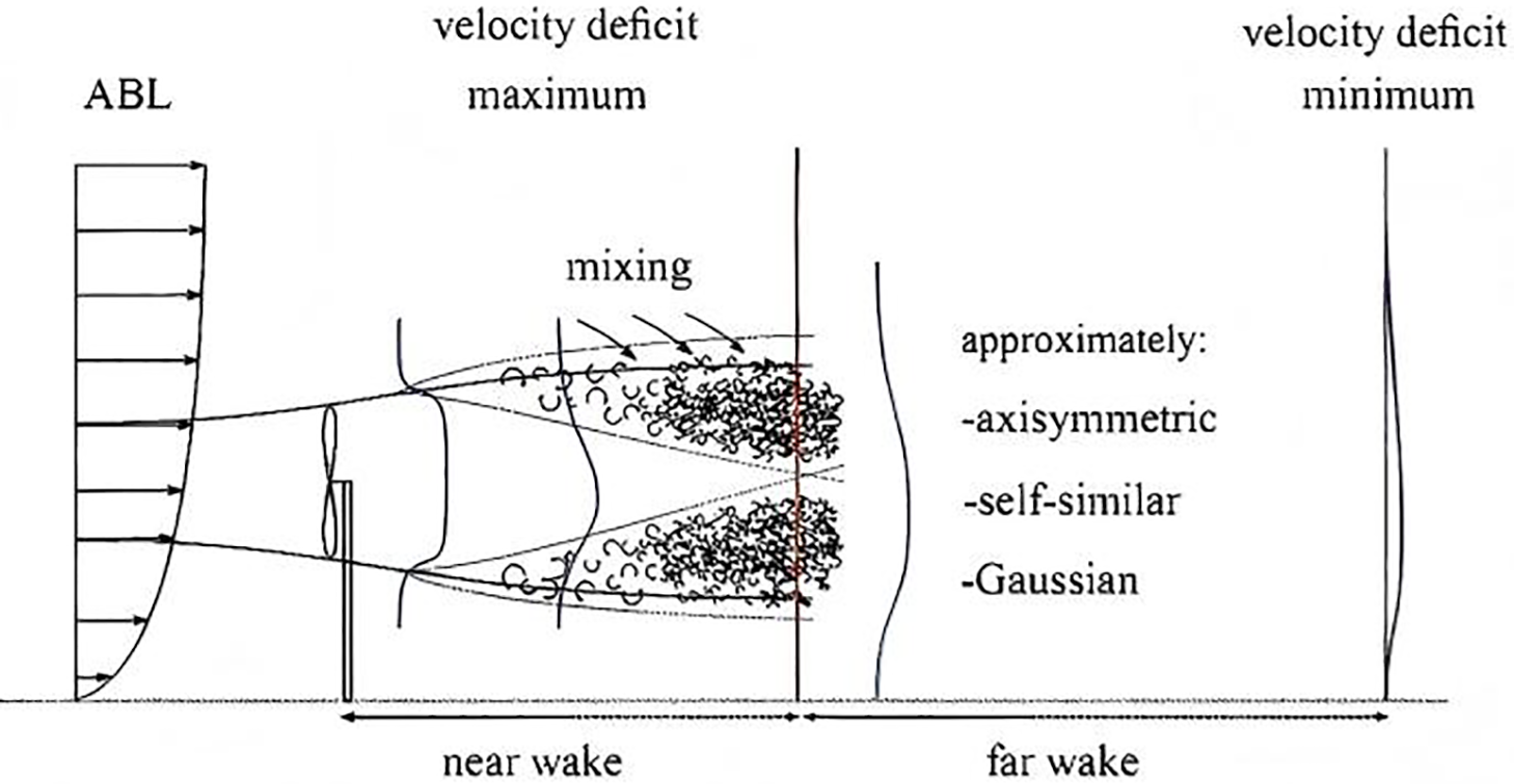
Figure 1: Schematic diagram of wind turbine wake

To address wake loss, the Active Wake Control (AWC) strategy has gained significant attention [6,7]. Among AWC technologies, which include axial induction control, wake redirection, and enhanced wake mixing, yaw-based control strategies have shown great potential [8]. This strategy intentionally creates a certain angle between the upstream wind turbine and the incoming wind. By yawing, the wake is laterally deflected, potentially reducing the direct impact on downstream turbines, thereby enhancing the overall power output of the wind farm [9]. To effectively design, analyze, and optimize this method, it is essential to rely on precise modeling and high-performance simulation tools.

The successful implementation of yaw-type AWC depends on several key factors. First, it is essential to accurately predict wake behavior, including the distribution of speed loss and wake deflection trajectories under yaw conditions. To achieve this, researchers have developed various wake models, ranging from classical analytical models like the Jensen model [10,11] and Gaussian model [12] to computationally intensive numerical simulation methods such as large eddy simulation (LES) [13,14]. Parametric models, such as the Floris (FLOw Redirection and Induction in Steady-state) model [15,16], offer a good balance between computational efficiency and simulation accuracy, making them suitable for developing control strategies. The Floris model can explicitly simulate wake deflection and the superposition effect of multiple wakes, often using Gaussian functions to describe speed loss [17].

Second, general wake models often require site-specific calibration to account for local topography, atmospheric conditions, and the characteristics of the wind turbines [16]. The key parameters determining wake expansion and deflection can vary significantly across different sites. Third, practical applications also face challenges related to the quality and availability of data from supervisory control and data acquisition (SCADA) systems. For example, the true north alignment (TNA) information, which serves as a reference for yaw angle measurements, may be inaccurate or missing, hindering the accurate interpretation of wind direction and yaw settings [18]. Finally, finding the optimal yaw angle combination for all wind turbines within a wind farm is a complex optimization problem, with objectives that are high-dimensional, nonlinear, and typically non-convex [19]. To address such complex issues, advanced modeling, simulation, and optimization techniques are required, taking into account various factors in the natural environment.

This paper addresses the interconnected challenges by proposing an integrated approach to optimize wind farm power output through yaw control, using a wind farm in northern Hebei, China, as a specific application. The method integrates practical data preprocessing techniques for TNA estimation, site-specific calibration of the Floris wake model, and robust optimization simulations based on the derivative-free NOMAD solver. This approach aims to enhance the energy capture of wind farms and can serve as a reference for constructing high-precision virtual wind farm environments.

Research on wind farm optimization, considering wake effects, has made significant progress. Early work primarily focused on static layout optimization [20]. With the development of active wake control (AWC) technology, particularly yaw control, the focus shifted to operational strategy optimization [21]. The Floris model [22], developed by NREL and its collaborators, has become a commonly used tool in AWC research due to its ability to effectively simulate wake deflection and high computational efficiency [17]. Subsequent extended models, such as FLORIDyn, further incorporate dynamic effects [23]. The effective application of these models requires a deep understanding and precise modeling of the wind farm’s natural environment. Optimization algorithms for yaw control range from gradient-based methods (which require analytical or adjoint gradients [19]) to heuristic algorithms and derivative-free methods [24]. Derivative-free methods, such as the Mesh Adaptive Direct Search (MADS) [25] algorithm (implemented in solvers like NOMAD [26]), are particularly suitable for handling complex, simulation-based ‘black box’ objective functions or noisy data, which are common in wind farm optimization problems. Such simulation optimization techniques are valuable for exploring and testing control strategies in virtual environments.

Despite significant progress, there are still shortcomings in integrating actual data processing, site-specific model calibration, and robust optimization simulation into a unified method validated by site data. Although the TNA error issue has been recognized [18], systematic estimation of TNA using operational data remains to be explored in the AWC context. Similarly, while the importance of model calibration is widely acknowledged, research on practical iterative calibration using data from Supervisory Control and Data Acquisition (SCADA) systems and integrating it into an optimization framework for validation needs to be enhanced. This study aims to address these gaps and contribute to the development of a more accurate wind farm virtual environment.

This article aims to fill these gaps through the following contributions:

1.    A practical simulation-assisted matching method based on normal distribution fitting has been developed and applied to estimate missing or uncertain true north alignment data of wind turbines from SCADA measurement data. This method leverages the consistency between simulated wake patterns and actual SCADA wind conditions/power data, identifying data segments that match specific simulation conditions to achieve a robust estimation of TNA.

2.    An iterative estimation method was designed to calibrate the key parameters of the Floris wake model (which affects the wake expansion rate) using the SCADA power data of the target power station (Jibei Wind Farm), so as to improve the prediction accuracy of the model for this specific site. This process also explored the dependence of the calibrated parameters on wind speed and wind turbines.

3.    The gradient-free NOMAD solver is applied and analyzed to determine the optimal yaw angle that can maximize the total power of a wind farm under specific wind conditions based on the calibrated Floris model.

Through a simulation case study based on the real operational data of an 11-turbine cluster at the Jibei Wind Farm, the advantages of the integrated method are demonstrated and quantified. The study clearly demonstrates that using site-specific model calibration in simulations can enhance yaw optimization performance. By selecting actual operational scenarios and calibrating with measured data, the study provides a solid simulation foundation for subsequent on-site verification.

The remainder of this paper is organized as follows: Section 2 provides a detailed explanation of the problem formulation and mathematical background, including the definition of angles and the structure of the wake model. Section 3 describes the proposed integrated method, which includes TNA estimation, Floris model calibration, and yaw angle optimization. Section 4 presents a case study using data from the Jibei Wind Farm and analyzes the simulation results. Section 5 summarizes the paper, highlighting the main findings and discussing future research directions, particularly the necessity of field validation.

2  Problem Formulation and Mathematical Background

This section formally defines the problem of wind farm yaw optimization and introduces the relevant mathematical concepts and models.

2.1 System Definition and Symbols

Consider a wind farm consisting of N wind turbines, where the layout is represented by the set of turbine indices NWF=1,2,…,N. Each turbine’s position (xi,yi,zh,i) is defined by its coordinates (eastward, northward, hub height). Each turbine has a rotor diameter Di and swept area Ai=πDi2/4. The wind farm operates under environmental wind conditions, characterized by free-stream wind speed U∞ (at a reference height), wind direction ϕ∞ (the angle measured clockwise from true north), and turbulence intensity I∞. Air density is denoted as ρ.

Precise definition of the angle is critical for wake modeling and control. The key angles are defined below and illustrated schematically in Fig. 2. The following definitions are adopted.

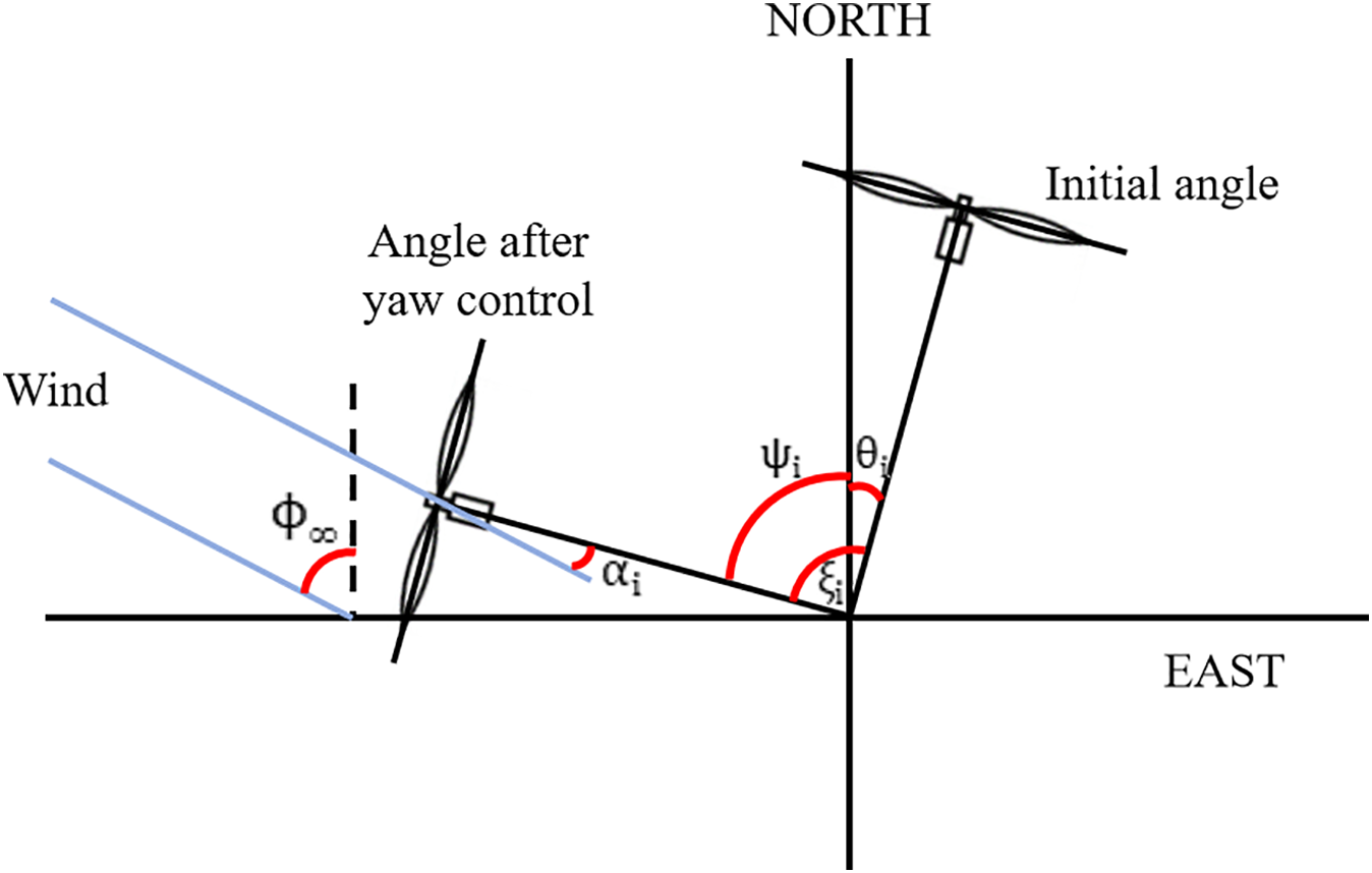
Figure 2: Schematic of angle definitions

θi: True north alignment angle of the wind turbine i. This is the reference angle between the turbine’s 0° yaw reading and true north.

ξi: The yaw angle reading from the SCADA system for wind turbine i, measured relative to its reference direction θi.

ψi: The absolute yaw direction of the rotor shaft for wind turbine i relative to true north. The calculation formula is as follows:

ψi=(ξi−θi).(1)

ϕ∞: The environmental wind direction (clockwise from true north), represents the free-stream wind condition, undisturbed by the wind farm. The local wind direction at each turbine, ϕlocal,i, is derived from ϕ∞ after accounting for the wake effects from upstream turbines.

αi: The relative wind direction angle measured by the hub wind vane reflects the relative relationship between the incoming flow direction and the wind turbine head cover.

ϕlocal,i: The effective local wind direction acting on the rotor of wind turbine i takes into account the wake effect. Under certain assumptions, this can be approximated by the measured angle and the calculation formula is as follows:

ϕlocal,i≈(ψi−αi).(2)

γi: The yaw angle deviation of the wind turbine i is the angle between the effective local wind direction and the rotor shaft direction of the wind turbine. The calculation formula is as follows:

γi=ψi−ϕlocal,i.(3)

Fig. 2 presents a simplified schematic for conceptual clarity. The yaw misalignment γi is approximately equal to the measured relative angle αi. Because this approximation is difficult to represent clearly in a diagram and would add unnecessary complexity, only αi is labeled. Furthermore, the diagram illustrates an upstream turbine where the local wind direction ϕlocal,i is assumed to be the same as the free-stream wind ϕ∞. It is important to note that for downstream turbines, ϕlocal,i will differ from ϕ∞ due to wake effects, which is a core element of the model.

2.2 Floris Wake Model

The Floris model [16,21] is used to predict wind fields within a wind farm. It calculates the speed loss and deflection caused by each wind turbine, and combines these effects to determine the local wind conditions (Ulocal,i,ϕlocal,i) for each downstream wind turbine. The model uses a Gaussian shape to represent the speed loss, and considers the wake deflection [15] caused by yawing.

The radial width σ of the wake is modeled as increasing linearly with downstream distance x, starting from the initial width at the effective starting point σ0 of the wake. The rate of this linear expansion (i.e., the slope relative to x/D) is influenced by environmental turbulence intensity I∞ and other factors ka and kb, which are parameterized by:

k=kaI∞+kbϕlocal,i.(4)

The cross-sectional and vertical wake widths (σy,σz) follow this growth rate, which may have different initial widths or dependence on yaw. Parameters ka and kb are crucial for accurately modeling the wake expansion rate at specific sites, and they require calibration. The Floris formula used in this study models the ratio of wake width to diameter as a linear increase with dimensionless downstream distance (x−x0)/D:

σy(x,γ)D=kyx−x0D+σy0(γ)D,(5)

σz(x)D=kzx−x0D+σz0D,(6)

where ky=kz=k, the effective wake origin is x0 and initial width are σy0,σz0. Floris employs a wake superposition method (such as the square sum of velocity losses) to integrate the effects of multiple wakes at downstream wind turbine locations [26].

The Floris model ultimately provides the following functions:

Ulocal,i=fspe(U∞,ϕ∞,{(xj,yj,zh,j)}j∈𝒩,{γj}j∈𝒩,I∞,𝒫wake∗),(7)

ϕlocal,i=fdir(U∞,ϕ∞,{(xj,yj,zh,j)}j∈𝒩,{γj}j∈𝒩,I∞,𝒫wake∗),(8)

where 𝒫wake∗ is the set of parameters of the calibrated wake model is shown, including ka∗ and kb∗.

2.3 Power and Thrust Model of Wind Turbine

The power Pi generated by the wind turbine i depends on the local wind speed Ulocal,i and its yaw angle γi. It uses the power coefficient CP,i of the wind turbine for modeling:

Pi=12ρAiCP,i(Ulocal,i,γi)(Ulocal,i)3.(9)

In yaw conditions, the power coefficient is usually related to the coefficient at zero yaw CP,curve,i(Ulocal,i) (derived from the power curve) by the cosine power law:

CP,i(Ulocal,i,γi)≈CP,curve,i(Ulocal,i)cosp⁡(γi),(10)

where p is an empirical index, usually between 1.88 and 3 [15].

Similarly, the thrust coefficient CT,i required for wake calculation depends Ulocal,i on and γi:

CT,i(Ulocal,i,γi)≈CT,curve,i(Ulocal,i)cosq⁡(γi),(11)

where CT,curve,i(Ulocal,i) is the thrust coefficient at zero yaw, q is another empirical index (for example, q≈1.88). While the optimization objective is power, the FLORIS wake model requires the thrust coefficient (CT) of each turbine to calculate the wake’s velocity deficit. The CT is therefore a critical intermediate variable.

Calculating local conditions (Ulocal,i,ϕlocal,i) requires knowing the thrust coefficient CT,j of upstream wind turbines, which in turn depends on their local wind speed. This interdependence needs to be solved iteratively in the wake model calculation to obtain a given set of yaw angle deviations γ.

2.4 Optimize Problem Modeling

The main objective is to find the yaw angle deviation vector γ∗=(γ1∗,…,γN∗) that maximizes the total power output 𝒫wake∗ of the wind farm under given environmental conditions (U∞,ϕ∞) and calibrated wake model parameters:

maxγPtotal(γ)=∑i=1NPi(γ|U∞,ϕ∞,I∞,Layout,𝒫wake∗),(12)

where the above formula is implicitly used by Pi(γ|…).

Optimization is subject to the operational constraints of allowable yaw angle deviation for each wind turbine:

γmin≤γi≤γmax∀i∈1,…,N.(13)

In this study, a typical restriction was applied as γmin=−30∘ and γmax=+30∘.

The optimization problem defined by the above formula shows the following characteristics:

•   Nonlinear: The objective function Ptotal(γ) is highly nonlinear. This arises from the cubic relationship between power and wind speed, the complex wake interactions, and the nonlinear turbine-specific curves for power and thrust (which internally affects the wake calculation).

•   Non-convex: The objective function is usually non-convex due to complex wake interactions and potential trade-offs, which may have multiple local optima.

•   High dimension: The number of decision variables is the number of wind turbines N in the controlled wind farm or cluster. For this case study, N=11.

•   Coupling: The yaw angle γj of a wind turbine affects the power output Pi of many downstream wind turbines through the wake model, resulting in strong coupling.

•   Black box evaluation: The evaluation of the total power output Ptotal(γ) requires the running of Floris simulation code. Gradient analysis may be difficult or expensive to obtain, making the derivative-free approach more applicable.

These features, especially the non-convexity of the problem and the black box nature of the problem, lead to the use of derivative-free optimization (Derivative-Free Optimization, DFO) algorithms, such as MADS (implemented by the NOMAD solver).

3  Problem Formulation and Mathematical Background

This section details the integrated workflow developed to address the yaw optimization challenges of wind farms. It includes data preprocessing for true north alignment estimation, on-site calibration of the Floris wake model, and the optimization process itself. The workflow integrates real-world operational data from natural environments with simulation models from virtual environments, aiming to enhance the power generation performance of wind farms in complex conditions through precisely calibrated model-driven optimization.

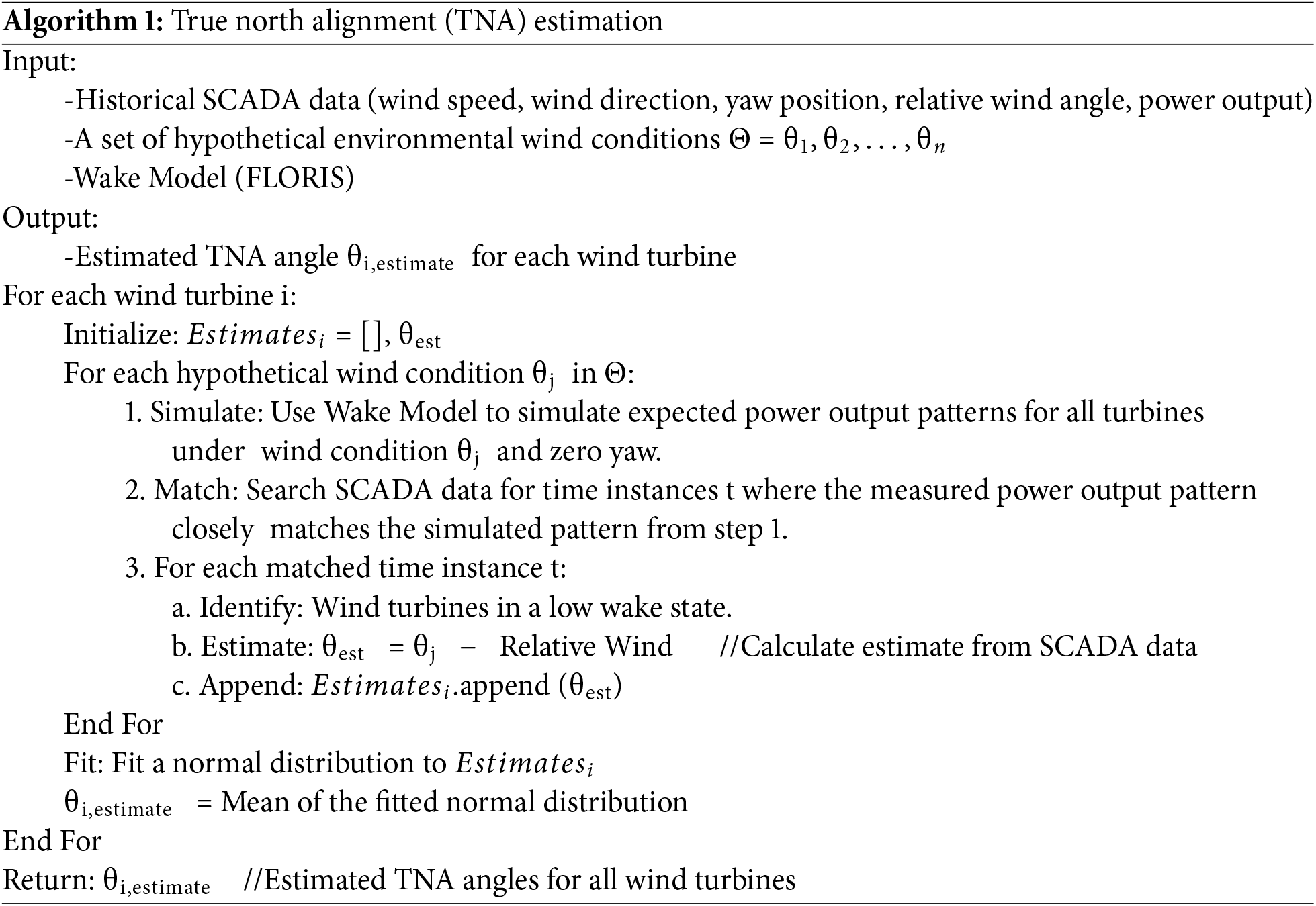
3.1 True North Alignment Angle Estimation

Accurate determination of the true north alignment angle θi of each wind turbine is essential for correctly associating the measured values based on the unit itself (ξi,αi) with the absolute wind direction ϕ∞ and calculating the actual yaw angle deviation γi. In practice, the value θi recorded at installation may be inaccurate or missing.

A data-driven simulation-assisted matching method has been proposed, utilizing historical SCADA data for estimating θi. The core concept relies on the relationship between the environmental wind direction, the absolute orientation of the wind turbine, and the measured relative wind angle αi. The effective local wind direction acting on the rotor of the wind turbine can be approximated as ϕlocal,i≈(ψi−αi) (based on the principle of hub sensors and ignoring certain effects, such as upwash or flow field distortions near the nacelle). For wind turbines operating in a relatively undisturbed flow field (for example, the front row of wind turbines upstream without wake effects), the local wind direction is approximately equal to the environmental wind direction, that is, ϕlocal,i≈ϕ∞. Therefore, for such data points, there exists an approximate relationship in Eq. (2).

If the ambient wind direction ϕ∞(t) at a given time t is known and the wind turbine is in a low wake state, by combining the relationships in Eqs. (1) and (2) and rearranging the terms, an estimate for θi can be obtained from SCADA data as follows:

θi,estimate(t)≈(ξi(t)−ϕ∞(t)−αi(t)).(14)

However, directly obtaining the instantaneous environmental wind direction at each wind turbine is challenging. Therefore, a simulation-assisted pattern matching method was adopted, which uses more detailed wake simulation models (such as FLORIDyn [22]) to generate expected spatial patterns, thereby combining natural environment observation data with virtual environment simulation results:

1.    Select a representative set of environmental wind conditions (U∞∗,ϕ∞∗) to cover the desired operating range.

2.    For each assumed environmental condition (U∞∗,ϕ∞∗), the comprehensive wake model (using FLORIDyn in this phase) is used to simulate the expected operational data space patterns for all wind turbines in the cluster. The simulation output includes the expected effective wind speed or corresponding power output (derived from the power curve) for each turbine under typical operating conditions, such as zero yaw angle deviation. This forms the baseline for expected behavior in a virtual environment.

3.    In the historical SCADA data, time instances t are searched to ensure that the relative effective wind speed or power output patterns of the wind turbines within the cluster closely match the simulated patterns (corresponding to a hypothetical scenario ϕ∞∗) from step 2. The matching criterion is to minimize the absolute difference between the measured values (such as effective wind speed calculated from SCADA power and power curves) and the simulated values. This step involves comparing the actual data from the natural environment with the simulation results from the virtual environment.

4.    For each matched time instance t, assume that the actual wind direction ϕ∞(t) is close to the assumed one ϕ∞∗. Additionally, for wind turbines in a low wake state during this matching scenario, their local wind direction ϕlocal,i(t) is approximately equal to the environmental wind direction ϕ∞(t). In these instances, data points of wind turbines significantly affected by the wake are excluded or given lower weight in the estimation of that specific time instance. Low wake conditions are identified by analyzing patterns consistent with undisturbed flow, such as wind speeds consistent with upstream wind turbines or wind towers, and by assessing the position of the wind turbine relative to the environmental wind direction. For selected low wake data points, the estimated value θi is derived using the formula ϕ∞(t)≈ϕ∞∗.

5.    Repeat steps 1–4 for multiple hypothetical environmental conditions (U∞∗,ϕ∞∗) and a large number of SCADA data sets to generate a distribution of estimates θi for each wind turbine i. The specific signals used in the analysis included active power, nacelle-based wind speed (at hub height), relative wind direction, and yaw position. Turbulence intensity was calculated based on the standard deviation of the nacelle wind speed.

6.    The estimated values of each wind turbine are fitted to a normal distribution. The mean of the fitted distribution µ is taken as the final robust estimate θi. This statistical method helps to average out noise, transient effects, and errors from individual matches or approximations. The standard deviation provides a measure of the uncertainty of the estimates.

This method leverages the patterns of multiple wind turbines and time instances to provide robust estimates θi, even in the presence of noisy SCADA data and uncertainties in instantaneous wind conditions. The accuracy of this step directly impacts the subsequent model calibration and optimization stages. The estimated TNA values for the wind turbines at the Jibei Wind Farm used in this study will be reported in Section 4. The overall process is illustrated in Algorithm 1.

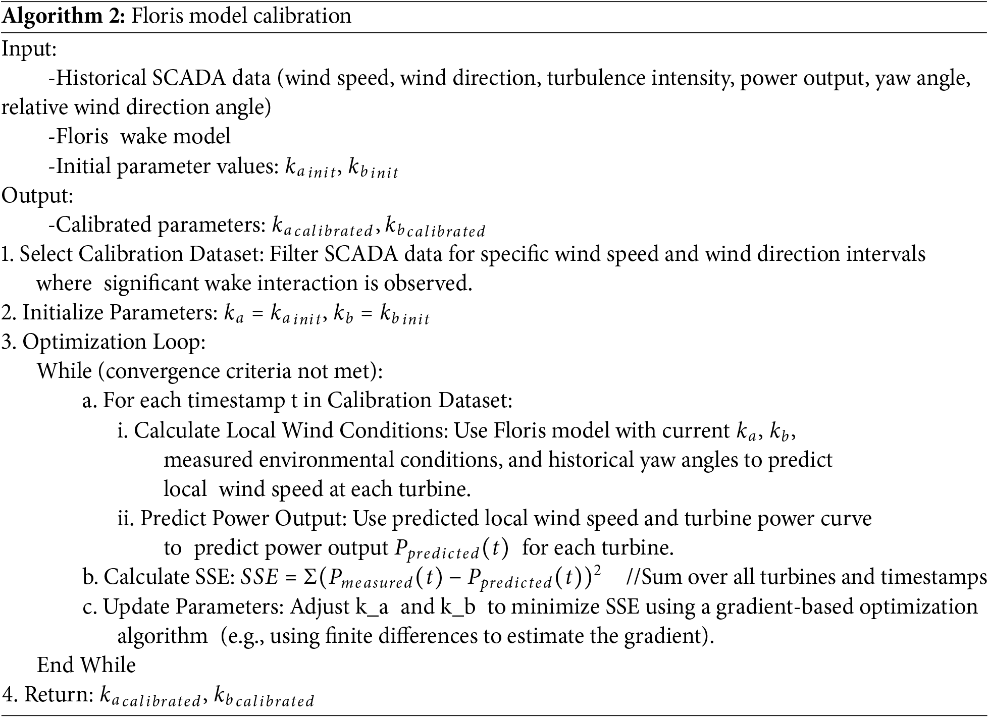
3.2 Calibration of Parameters of Floris Wake Model

The Floris model includes parameters that influence its predictions, particularly the wake expansion rate controlled by ka and kb, which is related to turbulence intensity I∞ and the baseline slope, as shown in Formula (4). These parameters can vary by site due to local topography, atmospheric conditions, and wind turbine characteristics. Additionally, these parameters may depend on wind speed and can differ among wind turbines due to variations in local microsite conditions or operational differences. This calibration process is a crucial step in integrating observed natural environmental behavior (SCADA data) into the virtual simulation model (Floris).

To enhance the accuracy of the Floris model in predicting wind power at the Jibei Wind Farm, historical SCADA data was used for calibration of ka and kb. The aim is to find the parameter values that minimize the difference between the power predicted by the calibrated Floris model and the actual power measured by SCADA on a representative dataset. The objective function is defined as the Sum of Squared Errors (SSE), as shown in Eq. (11). The focus is on minimizing the power prediction error because power is the ultimate optimization goal and is directly measured by SCADA.

The iterative estimation method adopted is based on the optimization approach to minimize the SSE objective function (11):

1.   Select a calibration dataset from the SCADA system, which includes timestamps t, measured environmental wind speed U∞(t) and direction ϕ∞(t) (such as from a wind tower or a designated reference wind turbine), turbulence intensity I∞(t)i, the measured power of each wind turbine Pi,meas(t), and the corresponding operating yaw angle ξi(t) and relative wind direction angle αi(t). Using the values estimated θi in Section 2.1, the historical yaw angle deviation is derived from the SCADA data based on the relationship between the environmental wind direction, the orientation of the wind turbines (θi+ξi), and the relative wind direction angle αi. The dataset is typically filtered to include specific wind speed and wind direction intervals where significant wake interaction has been observed.

2.   Initialize parameters ka and kb with default values (for example, ka=0.38371,kb=0.003678).

3.   The optimization algorithm is used to iteratively adjust ka and kb, and minimize the SSE objective function (11). A gradient-based approach can be used, where the gradient is derived numerically (e.g., using finite differences) or analytically (relative to parameters). In each iteration:

(1)   For the current parameter values (ka,kb), the Floris model is used to predict the power output Pi,pred(t,𝒫wake,θ∗) of each wind turbine i and all time stamps t in the calibration data set. This involves calculating the local wind conditions based on the current parameters, measured environmental conditions (U∞(t),ϕ∞(t),I∞(t)), and historical yaw angles (ξi(t),αi(t) derived from SCADA and θi estimated in (14)).

(2)   The total SSE is calculated according to Formula (11).

(3)   Update the parameters (ka,kb) according to the selected algorithm to reduce SSE (for example, using a calculated or approximate gradient).

4.   The iteration is terminated when the convergence criteria are met (e.g., SSE or relative improvement of parameter values is negligible, below the threshold, or maximum number of iterations is reached).

This process generates a set of calibration parameters 𝒫wake∗={ka∗,kb∗} that best represent the wake behavior observed at the Jibei site, aimed at minimizing power prediction errors. Calibration can be performed in wind speed intervals, and the resulting parameters may exhibit variations specific to the wind turbine, indicating potential local effects. When optimizing, appropriate calibration parameters are used based on the current environmental wind speed (for example, interpolation or using the nearest available wind speed interval, or specific values for the wind turbine if applicable). The overall process is illustrated in Algorithm 2.

3.3 Use NOMAD to Optimize Yaw Angle

Using the calibrated Floris model 𝒫wake∗ and accurate TNA(θi), the final step is to determine the optimal yaw angle γ∗ deviation under given environmental conditions (U∞,ϕ∞,I∞) to maximize the total wind farm power Ptotal(γ) while meeting operational constraints (formula). The optimized decision variable γi is the yaw angle deviation of each wind turbine i∈N. This optimization process, conducted in a calibrated virtual simulation environment, aims to find the optimal control strategy suitable for real-world (natural) conditions.

As discussed in Section 2.4, this is a nonlinear, non-convex, and high-dimensional optimization problem. While standard wake modeling tools often include built-in, gradient-based optimizers that are suitable for many applications, the specific formulation in this study presents unique challenges. The objective function is evaluated via a complex simulation chain that incorporates the site-specific, data-driven calibrated parameters. This process creates a “black-box” objective function with a complex landscape that can be challenging for gradient-based methods, which are often sensitive to numerical noise and may converge prematurely to a poor local optimum.

For this reason, the NOMAD (Nonlinear Optimization by Mesh Adaptive Direct Search) solver [27] was selected. NOMAD implements the MADS algorithm [28], a derivative-free method specifically designed for its robustness in solving such black-box problems. This choice prioritizes solution quality and reliability, as the algorithm does not require gradient information and uses dynamically refined grids to effectively explore the search space.

MADS is a derivative-free optimization method designed for black-box problems where gradients are unavailable or unreliable. The algorithm operates iteratively through two main steps: a Search step and a Poll step. In each iteration, it explores a set of points on a dynamically adjusted grid, or ‘mesh’, centered around the current best solution. The optional Search step allows for flexible exploration of the solution space using various heuristics. The mandatory Poll step, which guarantees the algorithm’s convergence properties, systematically generates a set of trial points on the mesh in specific directions. If a trial point yields a better objective function value, the iteration is deemed successful, the new point becomes the current best solution, and the mesh may be expanded. If no improvement is found in the Poll step, the iteration is unsuccessful, and the mesh is refined (i.e., its size is reduced) to focus the search more locally in the subsequent iteration. This adaptive process of exploring and refining the search space makes MADS robust and well-suited for complex, simulation-based optimization tasks like wind farm yaw control.

The implementation process involves defining a black-box function interface for the NOMAD call. This function takes a yaw angle deviation vector γ (the decision variable) as input. Inside this function, the calibrated Floris model is executed. This includes converting the required yaw angle deviation γ into the corresponding wind turbine orientation relative to north (absolute yaw direction ψi) based on the given environmental wind direction ϕ∞, the estimated TNA angle θ∗, and the relationship between local wind and environmental wind predicted by the Floris model. The model then predicts the local wind conditions Ulocal,i,ϕlocal,i for all wind turbines, considering their local wind speeds and deviations to calculate the power Pi of each wind turbine. The function returns the negative value of the total power −Ptotal(γ), aiming to maximize the total wind farm power by minimizing the loss. The lower and upper bounds (γmin,γmax) of each decision variable γi are provided to the NOMAD. The output is the optimal yaw angle deviation vector γ∗, designed to maximize the total wind farm power under given conditions using the calibrated model.

4  Case Study and Result Analysis

This section introduces the application of the proposed method to a cluster of 11 wind turbines at the Jibei Wind Farm, and analyzes the simulation performance of the yaw optimization strategy. The case study uses real natural environment data (SCADA records) to define the simulation scenario and calibrate the virtual simulation model (Floris), thereby evaluating the optimization effects under both real operational conditions and the virtual simulation environment.

4.1 Simulation Settings

4.1.1 Wind Farm Data

The study focuses on 11 wind turbines (numbered F178–F188) located at the Jibei Wind Farm near Zhangjiakou City, Hebei Province, China. The schematic diagram is shown in Fig. 3 and the geographical coordinates are shown in Table 1.

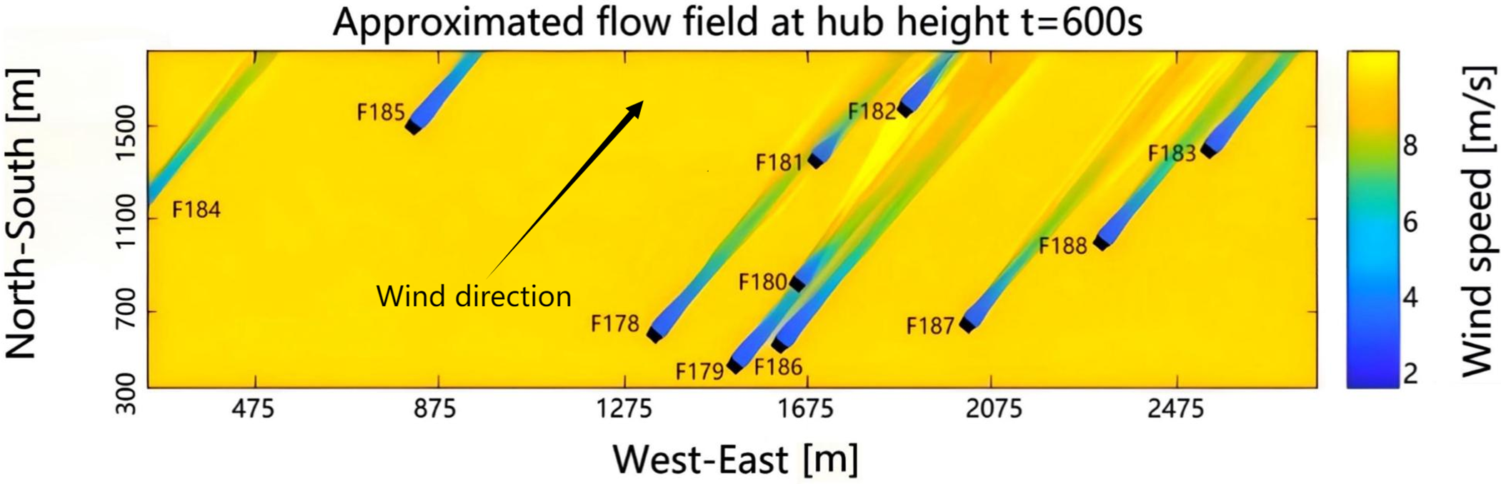
Figure 3: Schematic diagram of 11 wind turbine units in Jibei Wind Farm

The TNA estimates and model calibration were performed using SCADA data collected from the wind farm. Specifically, a six-month dataset, spanning from 01 January 2022, to 30 June 2022, was utilized. This dataset provided 10-min average values for each wind turbine, including wind speed, relative wind direction, yaw position, relative wind angle, and power output. The environmental turbulence intensity was also derived from this SCADA data. The true north alignment angle was estimated using the method described in Section 2.1, which was applied to this comprehensive dataset. Similar values were also obtained for other wind turbines. These estimated TNA values were used to derive historical yaw angle deviations from the SCADA data for calibration and optimization in the Floris simulation.

4.1.2 Wake Model and Calibration

The Floris wake model is implemented based on the modeling methods described in Section 2, including the dependence of the wake expansion slope on I∞,ka,kb. Key parameters ka and kb are calibrated using an iterative estimation method (Section 2.2), which is applied to a subset of SCADA data from the Jibei Wind Farm. This method categorizes data by wind speed and identifies conditions with significant wake effects. The calibration dataset aims to minimize the squared error between the predicted power from Floris and the measured power from SCADA. The initial values for calibration are set to the default values (ka=0.38371,kb=0.003678) of Floris. The calibration results show that the values of ka and kb vary with wind speed and exhibit differences among wind turbines. When the wind speed is approximately 10 m/s, the calibration process generates specific parameters for each wind turbine; for 11 wind turbines, the calibrated results of ka is approximately between 0.33 and 0.44, and the value range of kb is approximately between 0.0028 and 0.0035. Table 2 shows the calibration ka and kb values of 11 wind turbines at a wind speed of 10 m/s, obtained through this iterative calibration process. These calibrated, turbine-specific parameters are used in the optimization scenario at 10 m/s. For the 8 m/s scenario, the parameters calibrated for that wind speed range are utilized.

The value range for comparison, the optimization also uses a generic Floris parameter set that represents typical sites. These generic values are the default parameters for Floris: ka=0.38371 and kb=0.003678.

To validate the model’s accuracy, Fig. 4 provides a step-by-step comparison for a representative wake-inducing scenario, evaluating predictions against measured SCADA data for five key downstream turbines (F181–F185). The analysis breaks down the contributions of the proposed methodology. Five groups systematically build up the comparison to show how each component contributes to improving accuracy:

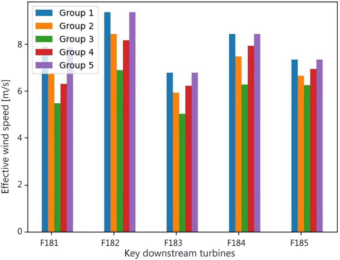
Figure 4: Comparison of predicted effective wind speeds for key downstream turbines, evaluating different model calibration stages against measured SCADA data

•   Group 1: “Measured SCADA Data”.

•   Group 2: “Generic Model” (Default TNA & Parameters).

•   Group 3: “TNA Correction Only”.

•   Group 4: “Parameter Calibration Only”.

•   Group 5: “Fully Calibrated Model” (TNA + Parameters), which is the proposed method.

The “Generic Model” (using default TNA and parameters) serves as the initial benchmark and exhibits a significant error. Interestingly, applying the “TNA Correction Only” makes the mismatch between the model and data larger for some turbines. Similarly, applying only “Parameter Calibration Only” results in a larger mismatch for the first two turbines (F181 and F182) and only slightly improves the model-to-data match for the other turbines. In contrast, the “Fully Calibrated Model”, which integrates both TNA estimation and site-specific parameter calibration, demonstrates the highest fidelity, aligning most closely with the measured data. This tiered comparison validates that the synergistic combination of both components in the integrated framework is essential for achieving a highly accurate predictive model.

4.1.3 Optimize the Solver

The NOMAD solver (version 3.9.1, invoked through PyNomad) was used to optimize the yaw angles of the 11 wind turbines. The objective function is the total power output of the 11 wind turbines, calculated using the Floris model with either general or site-specific calibration parameters. The decision variables are the yaw angle deviations γi of each of the 11 wind turbines, which are constrained within a specified range [γmin,γmax]=[−30∘,+30∘].

A standard NOMAD configuration was employed, and the process was limited to 1000 function evaluations to balance solution quality with computational cost. Each optimization run was executed on a desktop computer with an Intel Core i7-10700 CPU and 32 GB of RAM, and typically completed in 15–20 min.

4.1.4 Test Scenarios

In order to evaluate the effectiveness of yaw optimization, several specific environmental wind conditions were selected based on the analysis of SCADA data and wind turbine layout to identify scenarios with significant wake interaction. These scenarios were obtained by averaging SCADA data points falling within a narrow range of wind speed and wind direction:

•   Scenario 1: Wind direction ≈40∘ (interval 40∘±2∘), wind speed ≈8 m/s (interval 8±0.1 m/s)

•   Scenario 2: Wind direction ≈275∘ (interval 275∘±2∘), wind speed ≈8 m/s (interval 8±0.1 m/s)

•   Scenario 3: Wind direction ≈40∘ (interval 40∘±2∘), wind speed ≈10 m/s (interval 10±0.1 m/s)

•   Scenario 4: Wind direction ≈ 275° (interval 275∘±2∘), wind speed ≈10 m/s (interval 10±0.1 m/s)

•   Scenario 5: Wind direction 100.8∘, wind speed 10.07 m/s (representative operating conditions)

•   Scenario 6: Wind direction 240.3∘, wind speed 9.96 m/s (representative operating conditions)

For each scenario, the total simulated power output under three scenarios is calculated, which is consistent with the workflow evaluation framework:

•   Baseline: All wind turbines operate with zero yaw deviation (γi=0∘). The total power is simulated using the calibrated Floris model.

•   Optimization (General Model): The optimal yaw angle deviation γ∗ found by NOMAD using the Floris model with default parameters (ka=0.38371,kb=0.003678) is then used to simulate the total power at these angles using a calibrated model (representing the assumed site physical characteristics) to estimate the expected gain in a real-world scenario.

•   Optimization (Calibration Model): The optimal yaw angle deviation γ∗ found by NOMAD using the Floris model with site-specific calibration parameters (wind speed dependent, wind turbine specific). Then, the calibrated model is used to simulate the total power using these angles.

Comparisons 1 and 3 show the total simulation gain obtained using the full proposed workflow and calibration model. Comparisons 2 and 3 show the additional simulation gain specifically attributed to the use of the calibration model in optimization, assuming that the calibration model better represents the physical characteristics of the site.

4.2 Simulation Results and Discussion

4.2.1 Simulation Effects of Yaw Optimization (General Model)

Table 3 summarizes the simulated power gain achieved by using the Floris model with default parameters for yaw optimization in scenarios 1–4, which is relative to the zero yaw baseline (calculated using the calibration model).

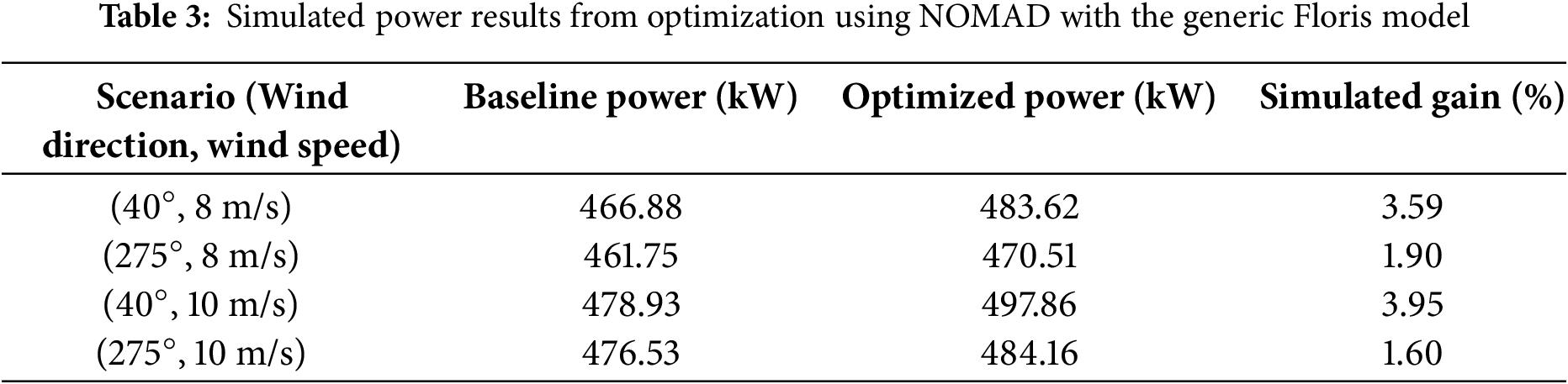
The results indicate that, when using a calibrated model for evaluation, the general Floris model simulating yaw optimization can enhance total power output compared to the zero yaw baseline. The simulation gain ranges from 1.60% to 3.95%, depending on the wind conditions. The higher gains observed at a 40° wind direction may be due to more direct wind turbine alignment, leading to stronger wake interactions, which offer greater potential for mitigation through wake guidance.

4.2.2 Model Calibration for Optimizing Simulation Benefits

To quantify the benefit of using a site-specific calibrated model, this study compares the outcomes of three distinct simulation scenarios. All scenarios are evaluated using the calibrated model to represent the physical reality of the site, ensuring a fair comparison:

•   Baseline Power: The power output with zero yaw deviation, calculated using the calibrated model. This represents the best estimate of the farm’s performance without active wake steering.

•   Optimized Power (General Model): The power output achieved using yaw angles that were optimized with generic FLORIS parameters. This shows the benefit of applying a non-site-specific control strategy.

•   Optimized Power (Calibrated Model): The power output achieved using yaw angles optimized with the site-specific calibrated parameters. This represents the full potential of the proposed method.

Table 4 presents the results of this comparison for scenarios 1–4. The “Additional Gain from Calibration” column isolates the performance improvement that is solely due to using the calibrated model during the optimization process, demonstrating the practical value of site-specific tuning.

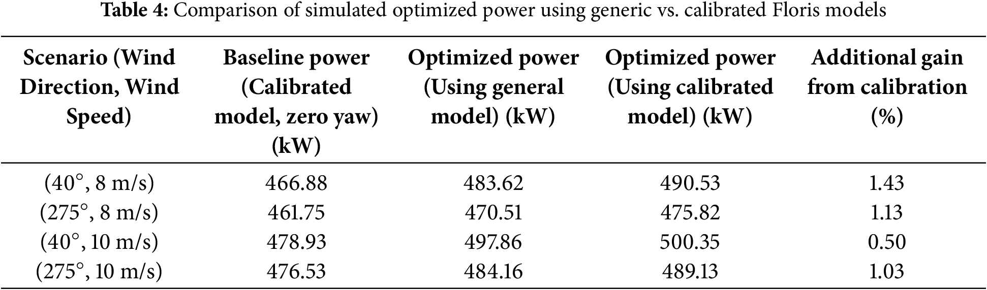
When both outcomes are evaluated using the calibrated model, using site-specific calibrated Floris model parameters 𝒫wake∗ within the NOMAD optimization framework consistently results in higher total power output simulations compared to using default parameters. In these scenarios, the additional simulation gain due to calibration during the optimization process ranges from 0.50% to 1.43%. This underscores the practical importance of calibrating the wake model to local conditions to maximize the effectiveness of AWC strategies. The calibrated model can more accurately predict the wake behavior of specific sites, enabling the optimizer to find better yaw angle solutions tailored to the site during simulations.

4.2.3 Simulation Results of Representative Scenarios

Table 5 shows the simulation optimization results using the calibrated model in two other representative operating scenarios (Scenario 5 and Scenario 6). The optimal yaw angle deviation found by NOMAD for these cases is shown in Table 6.

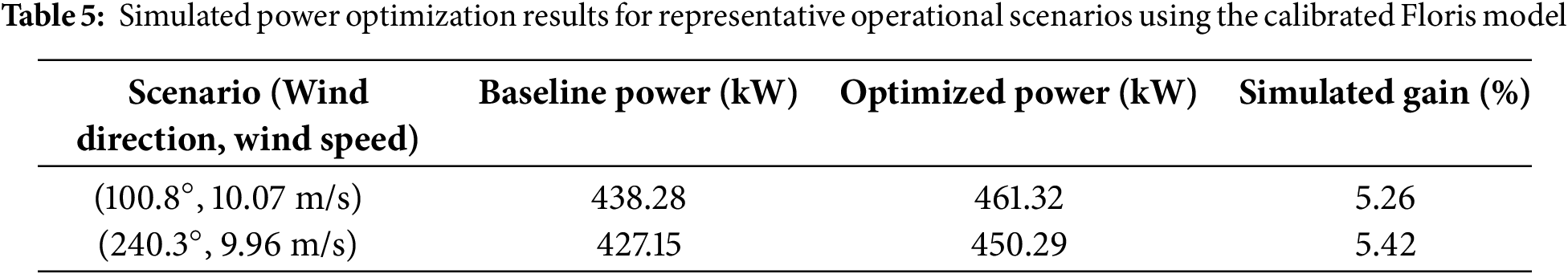
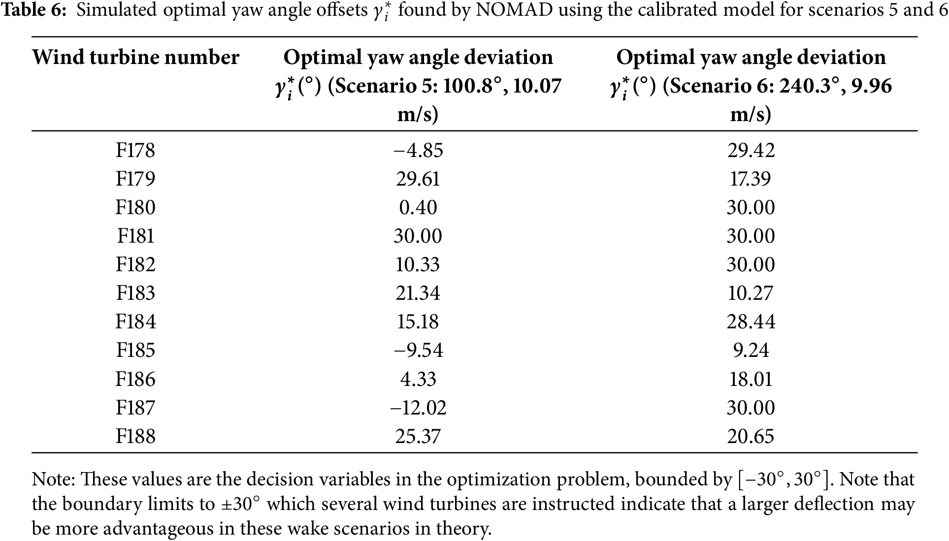
In these representative operational scenarios, the yaw optimization strategy using the calibration model achieved a significant simulation power gain of 5.26% and 5.42%, compared to the zero yaw baseline. Compared to scenarios 1–4, these higher gains may be due to the particularly strong and direct wake interactions within the cluster of 11 wind turbines caused by specific wind directions, offering greater potential for wake guidance improvements. The optimal yaw angle deviation (Table 6) indicates that different wind turbines are assigned different yaw angles, with upstream turbines typically yawing significantly (reaching the constraint ±30∘) to guide the wake away from multiple downstream turbines. Downstream turbines may be set to smaller yaw angles or zero yaw to maximize their capture of remaining wind resources. Several wind turbines were observed being instructed to the boundary limits ±30∘, suggesting that in these wake configurations, theoretically, a larger yaw angle could be more advantageous if not constrained by operational limitations.

4.3 Summary of Case Studies

The simulation case study using the data of Jibei Wind Farm shows the following simulation results within the framework of within the framework of a calibrated Floris model:

Compared with the baseline operation, using Floris model and NOMAD solver for yaw angle optimization in the simulation can effectively improve the total power output of wind turbine cluster.

Site-specific calibration of the Floris wake model parameters (ka,kb) significantly enhances the performance of yaw optimization in simulations, offering additional simulation power gains compared to using general model parameters. The magnitude of the simulation power gain achieved through yaw control depends on specific wind conditions (wind speed and direction) and the resulting wake interaction patterns. In test scenarios using the calibrated model, the observed simulation gain reached up to 5.4%.

The proposed overall method process, combined with TNA estimation, model calibration and robust optimization, provides a practical way to develop effective AWC strategy. The simulation results are promising and lay a solid foundation for future field verification.

These results validate the proposed method and highlight the importance of accurate, site-specific modeling when active wake control is used to maximize energy capture in a simulation.

5  Conclusion

This paper uses real operational data to define scenarios and calibrate models, with the simulation case study results clearly demonstrating the effectiveness of the proposed method in a simulation environment. Compared to baseline zero yaw operation, yaw angle optimization significantly boosts simulation power gain. Using site-specific calibration model parameters during the optimization process yields notably better simulation optimization results compared to using default parameters. When using the calibration model, the total simulation power gain observed under specific wake-induced wind conditions can reach up to 5.4%, highlighting the potential practical value of this integrated process after successful on-site implementation. This study confirms that accurate TNA estimation and site-specific model calibration are essential prerequisites for developing effective active wake control strategies based on wake models. The entire study demonstrates the value of integrating natural environmental data with virtual reality simulations in addressing complex engineering problems. Although this study provides valuable insights through simulations, it is based on steady-state assumptions and does not analyze the dynamic evolution of turbulence or the resulting structural loads. The true potential of active wake control can only be realized through a more holistic approach. To that end, our future work is focused on the development of a multi-objective Model Predictive Control (MPC) framework. This advanced strategy will incorporate wind condition forecasting and is designed to co-optimize for two competing goals: maximizing farm-level energy capture while simultaneously minimizing the fatigue loads on individual turbines. The findings in the present paper, particularly the validated, site-specific calibrated model, serve as a crucial foundation for this next-generation controller.

Acknowledgement: The authors would like to express their sincere gratitude to China South Power Grid Co., Ltd. for the generous support and funding provided for this research.

Funding Statement: This paper is supported by the Science and Technology Project of China South Power Grid Co., Ltd. under Grant No. 036000KK52222044 (GDKJXM20222430).

Author Contributions: Yang Liu: Data analysis, technical discussions. Lifu Ding: Algorithm design, manuscript writing, technical discussions. Zhenfan Yu: Technical discussions, experimental validation. Tannan Xiao: Code development, experimental testing. Qiuyu Lu: Data analysis, experimental validation. Ying Chen: Conceptual framework, project supervision. Weihua Wang: Technical discussions, experimental validation. All authors reviewed the results and approved the final version of the manuscript.

Availability of Data and Materials: Data available on request from the authors.

Ethics Approval: Not applicable.

Conflicts of Interest: The authors declare no conflicts of interest to report regarding the present study.

References

1. McCoy A, Musial W, Hammond R, Mulas Hernando D, Duffy P, Beiter P, et al. Offshore wind market report. 2024 edition. Golden, CO, USA: National Renewable Energy Laboratory (NREL); 2024. Report No.: NREL/TP-5000-90525. doi: 10.2172/2434294. [Google Scholar] [CrossRef]

2. Xu G, Yang M, Li S, Jiang M, Rehman H. Evaluating the effect of renewable energy investment on renewable energy development in China with panel threshold model. Energy Policy. 2024;187(12):114029. doi:10.1016/j.enpol.2024.114029. [Google Scholar] [CrossRef]

3. Ahmad S, Raihan A, Ridwan M. Role of economy, technology, and renewable energy toward carbon neutrality in China. J Econ Technol. 2024;2(1):138–54. doi:10.1016/j.ject.2024.04.008. [Google Scholar] [CrossRef]

4. Barthelmie RJ, Hansen K, Frandsen ST, Rathmann O, Schepers JG, Schlez W, et al. Quantifying the impact of wind turbine wakes on power output at offshore wind farms. J Atmos Ocean Technol. 2009;26(9):1848–61. doi:10.1175/2010JTECHA1398.1. [Google Scholar] [CrossRef]

5. Yang K, Kwak G, Cho K, Huh J. Wind farm layout optimization for wake effect uniformity. Energy. 2019;183:983–95. doi:10.1016/j.energy.2019.07.019. [Google Scholar] [CrossRef]

6. Knudsen T, Bak T, Svenstrup M. Survey of wind farm control-power and fatigue optimization. Wind Energy. 2015;18(8):1333–51. doi:10.1002/we.1760. [Google Scholar] [CrossRef]

7. Fleming P, King J, Dykes K, Simley E, Roadman J, Scholbrock A, et al. Initial results from a field campaign of wake steering applied at a commercial wind farm—part 1. Wind Energy Sci. 2019;4(2):273–85. doi:10.5194/wes-4-273-2019. [Google Scholar] [CrossRef]

8. Houck DR. Review of wake management techniques for wind turbines. Wind Energy. 2022;25(2):195–220. doi:10.1002/we.2668. [Google Scholar] [CrossRef]

9. Zong H, Sun E. Review of active wake control for horizontal axis wind turbines. Acta Aerodyn Sin. 2022;40(4):51–68. doi:10.7638/kqdlxxb-2021.0249. [Google Scholar] [CrossRef]

10. Jiménez Á., Crespo A, Migoya E. Application of a LES technique to characterize the wake deflection of a wind turbine in yaw. Wind Energy. 2010;13(6):559–72. doi:10.1002/we.380. [Google Scholar] [CrossRef]

11. Howland MF, Lele SK, Dabiri JO. Wind farm power optimization through wake steering. Proc Natl Acad Sci. 2019;116(29):14495–500. doi:10.1073/pnas.1903680116. [Google Scholar] [PubMed] [CrossRef]

12. Jensen NO. A note on wind generator interaction. Roskilde, Denmark: Risø National Laboratory; 1983. Report No.: Risø-M-2411. [Google Scholar]

13. Katic I, Højstrup J, Jensen NO. A simple model for cluster efficiency. In: European Wind Energy Association Conference and Exhibition; 1986 Oct 7–9; Rome, Italy. p. 407–10. [Google Scholar]

14. Bastankhah M, Porté-Agel F. A new analytical model for wind-turbine wakes. Renew Energy. 2014;70(10):116–23. doi:10.1016/j.renene.2014.01.002. [Google Scholar] [CrossRef]

15. Porté-Agel F, Wu YT, Lu H, Conzemius RJ. Large-eddy simulation of atmospheric boundary layer flow through wind turbines and wind farms. J Wind Eng Ind Aerodyn. 2011;99(4):154–68. doi:10.1016/j.jweia.2011.01.011. [Google Scholar] [CrossRef]

16. Göing J, Bartl J, Sætran L. A detached-eddy-simulation study: proper-orthogonal-decomposition of the wake flow behind a model wind turbine. J Phys Conf Ser. 2018;1049(1):012011. doi:10.1088/1742-6596/1104/1/012005. [Google Scholar] [CrossRef]

17. Bastankhah M, Porté-Agel F. Experimental and theoretical study of wind turbine wakes in yawed conditions. J Fluid Mech. 2016;806:506–41. doi:10.1017/jfm.2016.595. [Google Scholar] [CrossRef]

18. Farrell A, King J, Draxl C, Mudafort R, Hamilton N, Bay CJ, et al. Design and analysis of a wake model for spatially heterogeneous flow. Wind Energy Sci. 2021;6(3):737–58. doi:10.5194/wes-6-737-2021. [Google Scholar] [CrossRef]

19. Schreiber J, Bottasso CL, Bertelè M. Field testing of a local wind inflow estimator and wake detector. Wind Energy Sci Discuss. 2020;2020(3):1–24. doi:10.5194/wes-5-867-2020. [Google Scholar] [CrossRef]

20. Annoni J, Seiler P, Johnson K, Fleming P, Gebraad P. Evaluating wake models for wind farm control. In: American Control Conference; 2014 Jun 4–6; Portland, OR, USA; 2014. p. 2517–23. doi:10.1109/acc.2014.6858970. [Google Scholar] [CrossRef]

21. Mosetti G, Poloni C, Diviacco B. Optimization of wind turbine positioning in large windfarms by means of a genetic algorithm. J Wind Eng Ind Aerodyn. 1994;51(1):105–16. doi:10.1016/0167-6105(94)90080-9. [Google Scholar] [CrossRef]

22. Simley E, Fleming P, Girard N, Alloin L, Godefroy E, Duc T. Results from a wake-steering experiment at a commercial wind plant: investigating the wind speed dependence of wake-steering performance. Wind Energy Sci. 2021;6(6):1427–53. doi:10.5194/wes-6-1427-2021. [Google Scholar] [CrossRef]

23. NREL. FLORIS—FLOw redirection and induction in steady state. [cited 2025 Jan 1]. Available from: https://github.com/NREL/floris. [Google Scholar]

24. Doekemeijer BM, van der Hoek D, van Wingerden JW. Closed-loop model-based wind farm control using FLORIS under time-varying inflow conditions. Renew Energy. 2020;156(4):719–30. doi:10.1016/j.renene.2020.04.007. [Google Scholar] [CrossRef]

25. Becker M, Ritter B, Doekemeijer B, van der Hoek D, Konigorski U, Allaerts D, et al. The revised FLORIDyn model: implementation of heterogeneous flow and the Gaussian wake. Wind Energy Sci. 2022;7(6):2163–79. doi:10.5194/wes-7-2163-2022. [Google Scholar] [CrossRef]

26. Simley E, Fleming P, King J. Design and analysis of a wake steering controller with FLORIS. Wind Energy Sci. 2021;6(1):91–114. doi:10.5194/wes-5-451-2020. [Google Scholar] [CrossRef]

27. Audet C, Dennis JEJr. Mesh adaptive direct search algorithms for constrained optimization. SIAM J Optim. 2006;17(1):188–217. doi:10.1137/040603371. [Google Scholar] [CrossRef]

28. Le Digabel S. Algorithm 909: nOMAD: nonlinear optimization with the MADS algorithm. ACM Trans Math Softw. 2011;37(4):1–15. doi:10.1145/1916461.1916468. [Google Scholar] [CrossRef]