DC Disturbance Classification Method Based on Compressed Sensing and Encoder

1  Introduction

With the depletion of fossil energy sources, the adoption of new energy generation has become an inevitable trend in the development of the power industry. DC distribution networks have garnered significant public attention, and DC power supply has been implemented across multiple domains [1], gradually transforming the way electricity is utilized. However, DC distribution still confronts numerous challenges, such as power quality issues in DC grids. Power quality problems can adversely affect both industrial electricity usage and residential life [2]. Therefore, accurately classifying common DC power quality disturbance signals is crucial for addressing various related issues [3]. Given this context, effectively differentiating and precisely identifying DC power quality disturbance signals holds substantial importance.

Currently, research primarily focuses on the formation mechanisms and suppression methods of DC disturbances, with relatively limited exploration into DC disturbance classification methodologies. Both domestic and international studies have developed mature classification algorithms for AC power quality disturbance signals, offering valuable insights for the classification of DC disturbance signals [4]. Power quality disturbance classification methods generally combine signal feature extraction with classifiers [5], both of which are indispensable components. Feature extraction for disturbance signals typically employs techniques such as Short-Time Fourier Transform (STFT) [6], S-Transform [7], and Wavelet Transform [8]. Among these, STFT introduces a time-frequency localized window function to treat the signal within the window as stationary, obtaining the frequency spectrum of the signal over various time intervals through window movement. However, this method’s resolution is limited and unsuitable for signals with abrupt changes over short durations. The S-Transform provides rich time-frequency information and feature data but suffers from high computational complexity. Wavelet Transform analyzes power quality disturbance signals using wavelet windows, yet it remains susceptible to noise interference. Common recognition methods include Artificial Neural Networks (ANNs) [9], Support Vector Machines (SVMs) [10], and Decision Trees [11]. One approach [12] first extracts signal features by combining Fourier Transform and S-Transform to obtain a composite signal feature, subsequently inputting this into a multi-level vector machine for compound feature recognition. However, as the number of disturbance types increases and the data volume grows, training speed slows down significantly, and classification accuracy markedly decreases.

In summary, the quality of power quality disturbance signal classification heavily depends on feature extraction. The aforementioned feature extraction and classification methods may lose some critical information during the recognition and classification of power quality disturbances. However, deep learning offers promising solutions to these challenges. In recent years, deep learning has been widely applied across various fields, yielding remarkable results. Its application in the recognition and classification of AC power quality disturbance signals is emerging, and this approach can be extended to DC power quality disturbance signal recognition. Examples of such methods include Auto-Encoders (AE) and Deep Belief Networks (DBN). Reference [13] utilizes auto-encoders for power quality disturbance signal classification but struggles with noise interference. Reference [14] employs DBN for power quality disturbance signal classification, making it suitable for engineering applications but involving a complex process and long classification times.

To address issues such as large data volumes and poor recognition accuracy of power quality disturbance signals, this paper proposes a method that combines compressed sensing with Stacked Denoising Autoencoders (SDAE) for signal feature extraction and classification. The sparse vector obtained through compressed sensing is used to enhance the encoder model. The Root Mean Square Backpropagation (RMSprop) optimization algorithm is applied to improve network performance. This method leverages the constructed network model to extract features from power quality signals and ultimately classify them. Extensive simulation analyses demonstrate that the proposed method can accurately classify five common types of DC disturbance signals.

2  Establishment of the DC Electric Energy Index System and Disturbance Signal

2.1 DC Energy Index System and DC Voltage Class

Power quality issues are defined under IEC standards as deviations in the fundamental characteristics of a power supply system that prevent normal, uninterrupted, or interference-free electricity usage under standard operating conditions [15]. Specifically, any deviation in voltage or current parameters—such as amplitude, frequency, or waveform—from their specified values that causes equipment malfunction or failure constitutes a power quality problem.

Current research on DC power quality remains in its early stages, necessitating the adaptation of existing AC power quality frameworks. However, when classifying and defining DC power quality phenomena, it is critical to account for inherent differences between AC and DC systems. Ultimately, a comprehensive DC power quality index system is established, as depicted in Fig. 1.

Figure 1: DC energy quality index system

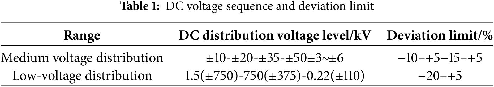
When formulating DC power quality evaluation standards, indices can be streamlined for specific application scenarios or voltage levels by considering interdependencies among indicators. This approach allows for the consolidation and simplification of metrics. According to the guidelines outlined in GB/T 35727 “Technical Specifications for Medium and Low Voltage DC Distribution Systems,” voltage classifications are categorized as follows: medium-voltage distribution spans ±1.5 kV to ±50 kV (3 kV to 100 kV line-to-line), while low-voltage distribution ranges from ±75 V to ±750 V (110 V to 1500 V line-to-line). The specific voltage classes and corresponding limit values are detailed in Table 1.

2.2 Common DC Power Quality Problems

In the process of DC distribution, issues related to frequency, phase, or reactive power do not arise. Currently, research on DC power quality problems is still in its infancy, and there is no unified standard for definitions and classifications. Therefore, it is necessary to refer to relevant AC power quality index systems while considering the differences between AC and DC systems to classify and define DC power quality signals [15]. Power quality problems can be categorized into two main types: event-based and variation-based. Event-based power quality problems include voltage sags, swells, and short-duration voltage interruptions. Variation-based issues encompass voltage fluctuations and DC voltage harmonics.

(1) DC voltage sag

Voltage sag is a common power quality phenomenon in DC distribution systems. It refers to a sudden decrease in the DC bus voltage to between 90% and 1% of the nominal voltage, which then returns to normal within a very short period. The primary causes of this phenomenon include DC bus grounding short circuits, abrupt changes in micro-source power, and the switching of DC loads [15].

The severity of voltage sag can be quantified by the magnitude of the voltage drop and its duration. Different electrical environments exhibit varying tolerances to voltage sag. Consequently, the concept of voltage sag depth is introduced for analyzing and evaluating the severity of DC voltage sag. This index can be represented by the following Formula (1):

MF% =Ud−Ud′UdcN×100%=usagUdcN×100%(1)

where: Ud is the actual voltage measured before the sag occurs, Ud′ is the actual voltage value at the measuring point after the sag occurs, usag is the difference between the actual voltage values at the measuring point before and after the sag occurs, and UdcN is the rated voltage of the DC bus.

(2) DC Voltage Short-Duration Interruption

This phenomenon occurs when the voltage of the DC bus drops to near zero for a short duration. The main causes of this issue include faults in the DC distribution system (e.g., short circuits between terminals), control failures (e.g., protection operation failures or errors during switching), and equipment failures (e.g., faults occurring in DC equipment between the positive and negative poles) [16].

(3) DC Voltage Swell

DC voltage swell refers to a sudden increase in line voltage during DC distribution, rising to more than 1.1 times the system’s rated voltage but typically not exceeding 1.8 times. The voltage quickly returns to normal within a short period, with the phenomenon usually lasting less than one minute. The causes of DC voltage swell include temporary voltage increases in distributed energy sources due to random changes in wind, sunlight, temperature, etc., and voltage transients occurring after fault-induced load shedding during the DC distribution process, followed by a recovery phase [17].

(4) DC Voltage Fluctuation

Given the limited capacity and power of DC distribution systems, which are not infinite sources, the voltage within the DC system can fluctuate due to the influence of distributed energy sources or high-power loads. DC voltage fluctuation refers to the random variation in voltage magnitude within the range of 0.9 to 1.1 times the rated voltage. Under normal conditions, DC voltage fluctuations do not contain fixed frequency components [17].

DC voltage fluctuations are typically characterized by two features: First, the voltage change rate is expressed as the ratio of the amplitude difference to the time difference between them, and the waveform within any sampling period (T_s) is analyzed. This can be represented by the following Formula (2):

ε=Udcmax−UdcminΔt×100% =UbΔt×100% (2)

where: Udcmax is the peak value of the DC voltage in the cycle, Umin is the valley value of the DC voltage in the cycle, Ub is the difference between the peak and valley of the fluctuation amplitude, and t is the time difference between them.

Second, Relative Voltage Fluctuation is defined as the ratio of the difference between the DC voltage peak and the trough over one period to the rated DC bus voltage, usually expressed as a percentage. It is given by the following Formula (3):

δ=Udcmax−UdcminUdcN×100% =UdUdcN×100% (3)

where: Udcmax is the peak value of DC voltage in this cycle, Udcmin is the trough value of DC voltage in this cycle, Ud is the difference between the peak and trough of the fluctuation amplitude, UdcN is the rated voltage of the DC bus, corresponding to the voltage level at the measurement place.

Voltage fluctuation primarily originates from four interconnected sources: interference propagating through AC grid interconnections, short-circuit faults occurring in AC-DC hybrid systems, recurrent switching operations of short-duration loads inducing DC-side perturbations, and inherent load variations at the consumer side.

(5) DC Voltage Harmonics

Although DC systems lack a fundamental frequency, studies confirm the presence of high-frequency components in DC distribution. Consequently, DC voltage harmonics are defined as sinusoidal waveforms superimposed on the nominal DC voltage at measurable amplitudes [18].

To measure and assess the magnitude and distortion of DC harmonics, concepts such as Harmonic Rate ((H_{\text{rate}})), Harmonic Amplitude ((H_{\text{amp}})), and Total Harmonic Distortion ((THD)) can be used. The calculation formulas for these concepts are given as follows:

{HRAh=AhAd×100%AH=∑h=1x(Ah)2THDA=AHAd(4)

where: A is the voltage, Ah is the root mean square value of the h-order harmonic voltage, and Ad is the root mean square value of the voltage at the test point on the DC side bus.

3  DC Power Quality Disturbance Data Processing Based on Compressed Sensing

3.1 Basic Principle of Compressed Sensing Theory

Compressed sensing (CS), introduced in 2006 by Terence Tao, Donoho D. L., and others [14], is a novel theoretical framework for signal acquisition and processing. This technique enables simultaneous signal acquisition and compression. The theory asserts that a signal compressible or sparsely representable in a specific transform domain can be mapped from high-dimensional to low-dimensional space via an observation matrix—one incoherent with the sparse transformation basis. An optimization algorithm then reconstructs the undersampled signal. The theoretical framework is illustrated in Fig. 2.

Figure 2: Compressed sensing theoretical framework

Three critical requirements govern the reconstruction of DC power quality disturbances via compressed sensing: (1) selection of an optimal sparse transformation basis for signal representation; (2) deployment of an observation matrix satisfying the Restricted Isometry Property (RIP) to sample the signal and acquire observation vectors from which sparse vectors are reconstructed; and (3) implementation of a suitable optimization algorithm for precise disturbance feature extraction.

3.2 Sparse Representation of Signals

The theoretical foundation of compressed sensing and its practical application rely on sparse signal characteristics. Truly sparse signals are uncommon in practice. DC power quality disturbance signals lack inherent sparsity; however, specific transformations can render them sparse, confirming their compressibility. A signal (x) of length (N) can be linearly represented by a set of basis functions as:

x=Ψθ(5)

where, Ψ is sparse basis, θ is (N-dimensional vector). Commonly used discrete sparse bases include the Discrete Fourier Transform (DFT), Discrete Wavelet Transform (DWT), and Discrete Cosine Transform (DCT) [19].

In [2], the sparsity characteristics of power quality signals were analyzed across different sparse bases. Experimental results demonstrated that the Discrete Fourier Transform (DFT) provided a more effective sparse representation. Consequently, to reduce computational complexity and leveraging the sparsity of power quality disturbance signals after transformation, this study adopts DFT as the sparse transformation basis.

3.3 Observation Matrix and Disturbance Signal Reconstruction

The observation matrix samples the signal to acquire observation vectors, enabling reconstruction of the original signal or sparse vector as shown in Formula (6).

Crucially, the observation matrix must satisfy the Restricted Isometry Property (RIP). Mathematical proofs establish that the observation matrix and sparse transformation basis must be mutually incoherent—a property fulfilled by matrices such as

y=Φx=ΦΨθ=Aθ(6)

where, Ψ is the sparse basis, θ is the sparse coefficient, Φ is the observation matrix (M×N), and A=ΨΦ is the sensing matrix.

The observation matrix must satisfy the Restricted Isometry Property (RIP). Mathematically, the observation matrix and sparse transformation basis must exhibit mutual incoherence—a sufficient condition for RIP compliance. The random Gaussian matrix is mathematically guaranteed to be incoherent with the Discrete Fourier Transform (DFT) basis. Consequently, this paper adopts the random Gaussian matrix as the measurement matrix for DC power quality disturbance signals [20], with the complete workflow illustrated in Fig. 3.

Figure 3: Schematic diagram of compressed sensing theory

The reconstruction algorithm recovers the disturbance signal using the observation matrix and sparse transformation basis. This paper adopts the Generalized Orthogonal Matching Pursuit (GOMP) algorithm for signal reconstruction. As an enhanced variant of the Orthogonal Matching Pursuit (OMP) algorithm, GOMP’s core innovation lies in drastically reducing iteration counts during sparse reconstruction—particularly effective under sparse sampling conditions—thereby minimizing runtime while accelerating sparse vector acquisition [21].

4  DC Power Quality Disturbance Classification Based on Stacked Denoising Autoencoder

4.1 Preprocessing of Raw Data

In MATLAB, five distinct types of DC power quality disturbances were generated, with each signal comprising 1500 samples. The disturbance types include DC voltage swell, DC voltage sag, DC voltage harmonics, DC voltage short-term interruption, and DC voltage fluctuation. For each disturbance type, 1200 samples were allocated to the training set, and the remaining 300 samples served as the test set. Through compressed sensing theory, sparse vectors were derived for all signals. These vectors subsequently formed a training set and a test set with sparse vectors as samples.

4.2 Construction of Stacked Denoising Autoencoder Model

A traditional autoencoder (AE) comprises two main components: an encoder and a decoder. It includes an input layer, hidden layers, and an output layer. As illustrated in Fig. 4, the encoder consists of the input layer and the hidden layer, whereas the decoder is composed of the hidden layer and the output layer. During the encoding process, the input signal (x) with dimension (d) passes through the input layer and reaches the hidden layer, where it is transformed into (h). The formula for this operation is as follows:

Figure 4: Autoencoder algorithm model

During encoding, the input signal x of d dimension reaches the hidden layer through the input layer, and the signal becomes h. The expression formula is as follows:

h=f(x)=s(Wx+B)(7)

where: W is the weight vector, B is the bias value, s is the activation function, and the expression is:

s(x)=11+e−y(8)

Decoding is the inverse operation of encoding. The hidden layer maps the signal h to the output layer through the transmission function g(h). The expression formula is as follows:

y=g(h)=s(W′h+B′)(9)

where, W′ is the weight vector, B′ is the bias value of the decoding process, and W=W′ is usually.

The error between the output layer and the input layer needs to reach the minimum value to extract the characteristics of the power quality signal. The calculation formula is:

L(x,y)=L(x,g(fθ(x)))(10)

where, L is the minimum mean square error.

Generally, stochastic gradient descent (SGD) is used to adjust network parameters to reduce reconstruction error. As shown in Eq. (11).

{W←W−l∂L(x,y)∂WB←B−l∂L(x,y)∂B}(11)

where, l is the learning rate; ∂L(x,y)/∂W is the partial derivative of L(x,y) with respect to the weight W; ∂L(x,y)/∂B means the partial derivative of L(x,y) with respect to B.

The principle of the denoising autoencoder (DAE) is based on the traditional autoencoder [22]. To prevent overfitting, the original signal x is perturbed, and the corresponding feature vector is extracted. At this point, the input signal becomes x~, and the perturbed signal can be interpreted as adding noise. This enhances the robustness of the encoder. The encoder model is illustrated in Fig. 5.

Figure 5: Noise reduction autoencoder model

Then it is encoded and decoded to get the signal:

z=g(fθ(x~))(12)

At this point, the error changes from L(x,g(fθ(x))) to L(x,g(fθ(x~))). However, in practical training, a single-layer Denoising Autoencoder (DAE) is insufficient for extracting features from DC power quality disturbance signals [22]. Therefore, it is advisable to stack multiple DAE layers to form a Stacked Denoising Autoencoder (SDAE) for network training. This multi-layer architecture can effectively extract features from the signal, and the extracted features are then used as input to the classifier [23].

In deep learning, it is often necessary to construct a loss function for the original network and then optimize it through algorithms to find the optimal parameter values that minimize the loss function [24]. The traditional Stacked Denoising Autoencoder (SDAE) typically employs Stochastic Gradient Descent (SGD) during the fine-tuning phase. With each iteration, SGD updates the parameters for every sample and generally converges quickly, enabling the model to escape poorer local minima. However, due to the large number of updates, SGD can cause the cost function to fluctuate significantly, leading to unstable convergence and negatively affecting the classification performance of the encoder. Therefore, this paper improves upon the traditional SDAE by replacing SGD with the Root Mean Square Propagation (RMSprop) optimization algorithm during the fine-tuning phase. RMSprop adjusts the learning rate based on the recent gradient history, which helps stabilize the learning process, reduces the likelihood of getting stuck in local minima, and enhances the overall classification accuracy of the encoder.

4.3 Encoder Classification Implementation Process

In this paper, the traditional stacked denoising autoencoder (SDAE) was improved. Instead of using stochastic gradient descent (SGD) to update network parameters, the root mean square propagation (RMSprop) optimization algorithm was employed during the fine-tuning stage to reduce the risk of falling into local minima. The training process is illustrated in Fig. 6.

Figure 6: The flow chart of DC energy mass disturbance classification for SDAE was improved

(1) In MATLAB Simulink, a large number of DC disturbance signals were generated.

(2) After compressed sensing processing, the signal was reconstructed while generating sparse vectors.

(3) To ensure that the signals had the same measurement scale, normalization was applied to all data using Formula (13). Finally, the dataset was divided into two parts: the training set and the test set.

xnor=(x−xmin)/(xmax−xmin)(13)

where, xnor,xmax,xmin respectively refer to the signal size obtained through normalization and the maximum value of the signal before normalization.

(4) The stacking denoising autoencoder model was constructed, and layer-wise unsupervised pre-training was performed. Due to the large sample size, the training sample M could be divided into several small batch data blocks of m, enabling successive training for improved efficiency. After iterative and layer-by-layer training, the network initialization weights W and bias values B were obtained. The specific training steps are as follows:

1) Assuming there are n hidden layers, the grouped data were trained starting from the first hidden layer;

2) DAE was used to calculate the weight value W and the bias value B, and then the network parameters were initialized;

3) If m<M, proceed to 2). If no, go to the next step;

4) If e<emax (number of iterations set), e=e+1 execute 2), otherwise execute the next step;

5) The weight of the trained NTH layer are saved to obtain the feature vector of the NTH layer, which is used as the training sample of the n + 1 layer.

6) If n<nmax (number of hidden layers), e=e+1 perform 1). If this condition is not met, the training is over.

(5) For parameter fine-tuning, this paper employs a top-down small-batch RMSProp optimization algorithm to fine-tune the weight and bias values of the initial network parameters until the preset number of iterations is reached. The process is as follows:

1) Set the global learning rate l, decay rate ρ, initialize the cumulative variables r1=0,r2=0;

2) Randomly select small batch data of m samples from the training set, and use the error loss function to get the gradient of weight and bias value;

w←1m∂∑i=1m(yi−f(W,B)(xi))2∂Wb←1m∂∑i=1m(yi−f(W,B)(xi))2∂B(14)

3) Calculate the cumulative square gradient, as shown in Eq. (15).

{r1=ρr1+(1−ρ)w⊙wr2=ρr2+(1−ρ)b⊙b(15)

Note: ⊙ is the product symbol.

4) Update the weight and bias values of the encoder, as shown in Eq. (16).

{W=W−lr1⊙wB=B−lr2⊙b(16)

5) When the number of iterations reaches the set value, the operation will stop. If this condition is not met, perform 2) and continue parameter fine-tuning;

6) Keep the trained network well and test the classification performance of the encoder on the test set. Mean squared error (MSE) is used to evaluate the performance of the encoder.

MSE=1m∑i=1m(q(xi)−p(xi))2(17)

where: p(xi) is the data distribution predicted by the encoder; q(xi) is the real data distribution; m is the number of samples.

5  Experiment and Simulation

This paper selects five common types of DC power quality disturbance signals, as introduced in Section 1, for classification. To collect data and perform subsequent disturbance recognition and classification, it is necessary to construct a DC distribution simulation model. Therefore, MATLAB/SIMULINK is employed to model the DC distribution network, as illustrated in Fig. 7, and to generate the corresponding disturbance signals. The simulation results indicate that DC voltage sags can be caused by factors such as DC bus ground faults, sudden changes in micro-source power, and switching of DC loads; DC voltage short interruptions are triggered by inter-pole faults; DC voltage swells are induced by sudden reductions in AC/DC loads or random variations in distributed power sources due to environmental factors like wind, light, and temperature; DC voltage fluctuations occur due to large-power loads and the repeated startup and shutdown of short-time operating devices; DC voltage harmonics are caused by three-phase voltage asymmetry on the AC side of the DC distribution network. Meanwhile, the disturbance signals processed based on sparse vectors are fed into the encoder model for experimental simulation.

Figure 7: DC distribution network model diagram

5.1 Simulation Based on Compressed Sensing

The DC power quality signals obtained in Section 1 are simulated and analyzed using compressed sensing. Figs. 8 and 9 illustrate the reconstructed signals and sparse vectors corresponding to DC voltage fluctuations, DC voltage harmonics, and DC voltage sag. From the waveform graphs of the three sparse vectors, it is evident that the reconstructed signals generated by compressed sensing exhibit a small reconstruction error. Additionally, the sparse vectors, which contain numerous zero elements, significantly reduce the data volume. This clearly demonstrates that the sparse vectors preserve rich features of the original signals, thereby facilitating subsequent disturbance signal classification.

Figure 8: Reconstructed waveforms of several DC disturbance signals

Figure 9: Sparse vectors of several DC disturbance signals

5.2 Selection of the Number of Hidden Layers and Neurons

For stacked denoising autoencoders (SDAE), selecting the appropriate number of hidden layers and neurons is critical for achieving optimal disturbance recognition and classification results. In this study, a two-layer stacked denoising autoencoder is employed to train the samples. The number of neurons in each layer is determined based on the evaluation of Mean Squared Error (MSE). Initially, the number of neurons in the first hidden layer is identified by minimizing the MSE. Once the optimal number of neurons is established, the number of neurons in the second hidden layer is similarly determined through optimization of the MSE. When the number of hidden layers exceeds two, the MSE value increases, indicating that adding more layers leads to information loss and an increase in error. Consequently, having too many hidden layers does not yield better training results. Fig. 10 depicts the relationship between the number of hidden layers and neurons. The optimal number of neurons for each layer is found to be 300 and 100, respectively.

Figure 10: Selection of optimal number of neurons

5.3 Noise Resistance Performance Evaluation

In this study, Gaussian white noise with a mean of 0 and variance of 1 is added to the DC disturbance signals without noise. The Signal-to-Noise Ratios (SNR) of the added Gaussian white noise are 20, 30, and 40 dB, respectively, as the “damaged” signals. A two-layer stacked denoising autoencoder model is trained with the first and second hidden layers containing 300 and 100 neurons, respectively, and the number of iterations is set to 1000.

As shown in Fig. 11, when no Gaussian white noise is added, both the original signal and the sparse vector achieve good recognition performance for the DC power quality disturbance signals. After adding Gaussian white noise, due to the robustness of the DAE, the classification accuracy improves. At an SNR of 30 dB, the accuracy of both the original signal and sparse vectors reaches the maximum value, with minimal difference between them. As the SNR of the Gaussian white noise increases, it begins to interfere with the original signal, causing a slight decrease in classification accuracy. However, the accuracy remains comparable to that of traditional encoders. In summary, adding an appropriate amount of Gaussian white noise still results in good recognition performance.

Figure 11: The recognition accuracy of Gaussian white noise for disturbance signal

5.4 Evaluation of Network Performance

To evaluate the classification performance of the network, a Mean Squared Error (MSE) graph is plotted. A smaller minimum MSE value indicates superior classification performance. As depicted in Fig. 12, as the number of training epochs increases, the MSE value progressively decreases. For the original data, the MSE stabilizes after approximately 30 epochs, reaching its minimum at the 35th epoch. In contrast, the MSE for the sparse vector exhibits minimal change after the 15th epoch and stabilizes by the 20th epoch. Ultimately, both approaches achieve stable error values, with the sparse vector attaining the minimum MSE. This suggests that the sparse vector effectively reduces network complexity and conserves training time.

Figure 12: Network performance evaluation

5.5 Comparison with Other Disturbance Classification Methods

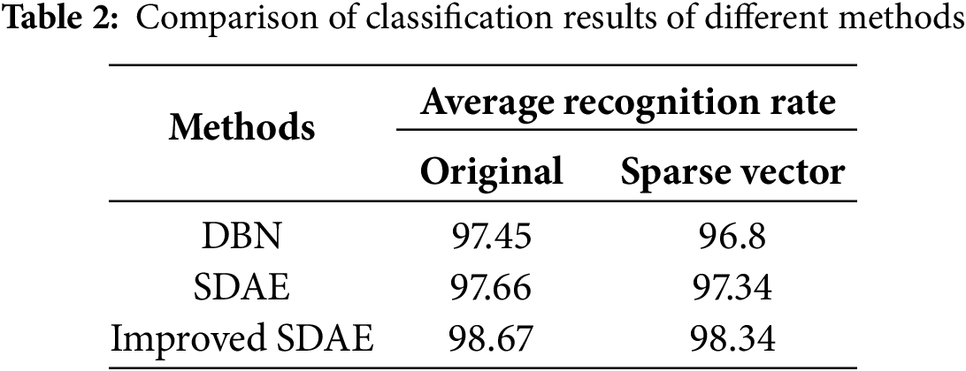
To further validate the performance of the classification method proposed in this study, its classification accuracy is compared with that of Deep Belief Networks (DBN) [14] and traditional Stacked Denoising Autoencoders (SDAE), as shown in Table 2. From the table, it can be observed that when the input signal corresponds to either the original data or the sparse vector, the classification accuracy of SDAE surpasses that of DBN. Moreover, the improved SDAE achieves higher classification accuracy relative to the conventional SDAE. These results underscore the efficacy of the proposed method in classifying DC power quality disturbance signals. The comparison outcomes are presented in Table 2.

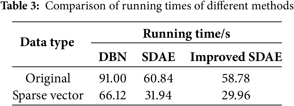
To verify that the improved Stacked Denoising Auto-Encoder (SDAE) has a shorter testing time, three classification methods were also compared. As can be seen from Table 3, when classifying DC power quality disturbance signals, the running time of the Stacked Denoising Auto-Encoder is significantly reduced compared with that of the Deep Belief Network (DBN). The improved encoder also shows a slight speed improvement. Especially when the sparse vector is used as the data sample set, even less time is required. Although under the same conditions, the accuracy is slightly lower than that of the original data, the classification time of the sparse vector is significantly reduced. Considering all factors, the classification method proposed in this paper is feasible for handling DC power quality disturbance signals.

6  Conclusion

The proposed method for identifying and classifying DC power quality disturbances combines Compressed Sensing (CS) with a Stacked Denoising Autoencoder (SDAE). The key findings are summarized as follows: First, DC power quality disturbance signals are processed using compressed sensing, where: the Discrete Fourier Transform (DFT) basis is employed for signal sparsification, A Gaussian matrix acts as the measurement matrix, and the Generalized Orthogonal Matching Pursuit (gOMP) algorithm performs sparse vector reconstruction. The resulting sparse vectors preserve the essential signal characteristics while significantly reducing data storage demands, thereby providing a reliable basis for subsequent classification. Second, the proposed method effectively addresses key limitations of traditional neural networks, including limited learning capacity and susceptibility to interference. By enabling efficient extraction of high-level feature representations from data, it significantly improves classification performance. Third, we implement an innovative SDAE network architecture integrated with RMSprop (Root Mean Square Propagation) optimization during training. The RMSprop algorithm dynamically adjusts network parameters, effectively reducing the likelihood of convergence to local optima. Through comprehensive simulation analyses—employing both raw signals and compressed sparse vectors as inputs—the proposed SDAE demonstrates superior capability in extracting discriminative features from DC power quality disturbances compared to conventional approaches. This methodological advancement yields significant improvements in both classification accuracyand computational efficiency.

This research offers insights into the identification and classification of DC power quality disturbance signals. Future research should focus on how to effectively implement this method in real-world power grid applications.

Acknowledgement: Not applicable.

Funding Statement: This research was funded by the National Natural Science Foundation of China (52177074).

Author Contributions: The authors confirm their contribution to the paper as follows: study conception and design: Huanan Yu, Jian Wang; data collection: Xiang Zhang; analysis and interpretation of results: Huanan Yu, Xiang Zhang; draft manuscript preparation: Xiang Zhang, Huanan Yu. All authors reviewed the results and approved the final version of the manuscript.

Availability of Data and Materials: The authors confirm that the data supporting the findings of this study are available within the article. And the additional data that support the findings of this study are available on request from the corresponding author, upon reasonable request.

Ethics Approval: Not applicable.

Conflicts of Interest: The authors declare no conflicts of interest to report regarding the present study.

Nomenclature

References

1. Yu L, Liu P, Li Y, Luo J. Research on new electric power data center based on DC power supply and distribution technology. In: 2022 IEEE International Conference on Power Systems and Electrical Technology (PSET); 2022 Oct 13–15; Aalborg, Denmark: IEEE; 2022. p. 297–302. doi:10.1109/PSET56192.2022.10100360. [Google Scholar] [CrossRef]

2. Li K, Cong S. State of the art and prospects of structured sensing matrices in compressed sensing. Front Comput Sci. 2015;9(5):665–77. doi:10.1007/s11704-015-3326-8. [Google Scholar] [CrossRef]

3. Gangatharan S, Rengasamy M, Elavarasan RM, Das N, Hossain E, Sundaram VM. A novel battery supported energy management system for the effective handling of feeble power in hybrid microgrid environment. IEEE Access. 2020;8:217391–415. doi:10.1109/access.2020.3039403. [Google Scholar] [CrossRef]

4. Hirose K, Shimozato A, Konno N, Murakami S, Nakao M. Status and challenges of energy efficiency & conservation using DC power technologies in Japan. In: 2024 13th International Conference on Renewable Energy Research and Applications (ICRERA); 2024 Nov 9–13; Nagasaki, Japan: IEEE; 2024. p. 1844–9. doi:10.1109/ICRERA62673.2024.10815343. [Google Scholar] [CrossRef]

5. Das D, Kumar C. Smart transformer based ship microgrid system. In: 2023 11th National Power Electronics Conference (NPEC); 2023 Dec 14–16; Guwahati, India: IEEE; 2023. p. 1–6. doi:10.1109/NPEC57805.2023.10384947. [Google Scholar] [CrossRef]

6. Wang R, Zhang S, Li N, Wang H, Li J. Research on distributed photovoltaic microgrid system based on dual-output T-type three-level converter. IEEE Access. 2024;12:142883–98. doi:10.1109/access.2024.3471784. [Google Scholar] [CrossRef]

7. Li P, Zhang H, Xiang W, Jia Q. A fast adaptive S-transform for complex quality disturbance feature extraction. IEEE Trans Ind Electron. 2023;70(5):5266–76. doi:10.1109/TIE.2022.3189107. [Google Scholar] [CrossRef]

8. Liu D, Zhu W, Wang Y, Chang Z, Xie K, Wang S. Power quality transient disturbances detection system based on Db5 wavelet. J Phys Conf Ser. 2023;2564(1):012010. doi:10.1088/1742-6596/2564/1/012010. [Google Scholar] [CrossRef]

9. Kankale R, Paraskar S, Jadhao S. Classification of power quality disturbances in emerging power system using S-transform and support vector machine. In: 2021 IEEE 2nd International Conference on Electrical Power and Energy Systems (ICEPES); 2021 Dec 10–11; Bhopal, India: IEEE; 2021. p. 1–6. doi:10.1109/ICEPES52894.2021.9699673. [Google Scholar] [CrossRef]

10. Aziz S, Khan MU, Abdullah, Usman A, Mobeen A. Pattern analysis for classification of power quality disturbances. In: 2020 International Conference on Emerging Trends in Smart Technologies (ICETST); 2020 Mar 26–27; Karachi, Pakistan: IEEE; 2020. p. 1–5. doi:10.1109/ICETST49965.2020.9080722. [Google Scholar] [CrossRef]

11. Guo F, Li J, Xu X, Zhu Y, Luo X, Qian W. Classification of transient power quality disturbances based on digital image processing techniques. In: 2023 8th International Conference on Power and Renewable Energy (ICPRE); 2023 Sep 22–25; Shanghai, China. p. 492–8. doi:10.1109/ICPRE59655.2023.10353758. [Google Scholar] [CrossRef]

12. Wang Y, Peng HP, Mo WX, Luan L, Xu Z. A local density clustering based method for disturbance source identification of power quality in distribution systems. In: 2021 International Conference on Power System Technology (POWERCON); 2021 Nov 8–11; Haikou, China. p. 1980–5. doi:10.1109/POWERCON53785.2021.9697635. [Google Scholar] [CrossRef]

13. Feng Z, Di L, Xiao QC, Ying W. Classification of multiple power quality disturbances based on CNN-BiLSTM-Attention. J Appl Sci Eng. 2024;27(7):2827–36. doi:10.6180/jase.202407_27(7).0007. [Google Scholar] [CrossRef]

14. Cheng L, Wu Z, Xuanyuan S, Chang H. Power quality disturbance classification based on adaptive compressed sensing and machine learning. In: 2020 IEEE Green Technologies Conference (GreenTech); 2020 Apr 1–3; Oklahoma City, OK, USA: IEEE; 2020. p. 65–70. doi:10.1109/greentech46478.2020.9289735. [Google Scholar] [CrossRef]

15. Liao JQ, Zhou NC, Wang QG, Li CY, Yang J. Definition and correlation analysis of power quality index of DC distribution network. Proc CSEE. 2018;38(23):6847–60,7119. (In Chinese). doi:10.13334/j.0258-8013.pcsee.181276. [Google Scholar] [CrossRef]

16. Guerrero JM. IEC 62040-3 and IEEE, 1547 standards for DC power quality in UPS systems. Elect Power Syst Res. 2018;163:1–12. doi:10.1016/j.epsr.2018.06.012. [Google Scholar] [CrossRef]

17. Liserre M, Blaabjerg F. DC microgrid power quality: state-of-the-art and future trends. Renew Sustain Energ Rev. 2020;130:110594. doi:10.1016/j.rser.2020.110594. [Google Scholar] [CrossRef]

18. Brenna M. Characterization and mitigation of voltage ripple in DC systems. Int J Elect Power. 2020;123(2):106567. doi:10.1016/j.ijepes.2020.106567. [Google Scholar] [CrossRef]

19. Candes EJ, Romberg J, Tao T. Robust uncertainty principles: exact signal reconstruction from highly incomplete frequency information. IEEE Trans Inf Theory. 2006;52(2):489–509. doi:10.1109/TIT.2005.862083. [Google Scholar] [CrossRef]

20. Mendelson S, Pajor A. Random matrices and sub-Gaussian sensing in compressed sensing. J Eur Math Soc. 2018;20(9):2113–52. doi:10.4171/JEMS/789. [Google Scholar] [CrossRef]

21. Wang J, Kwon S, Shim B. Generalized orthogonal matching pursuit. IEEE Trans Signal Process. 2012;60(12):6202–16. doi:10.1109/TSP.2012.2218810. [Google Scholar] [CrossRef]

22. Syamsudin M, Chen CI, Berutu SS, Chen YC. Efficient framework to manipulate data compression and classification of power quality disturbances for distributed power system. Energies. 2024;17(6):1396. doi:10.3390/en17061396. [Google Scholar] [CrossRef]

23. Zhou N, Zhang Y, Li X. Sparse stacked denoising autoencoder forrobust feature extraction. Neural Netw. 2021;138(11):124–35. doi:10.1016/j.neunet.2021.02.005. [Google Scholar] [CrossRef]

24. Liu Y, Jin T, Mohamed MA, Wang Q. A novel three-step classification approach based on time-dependent spectral features for complex power quality disturbances. IEEE Trans Instrum Meas. 2021;70:3000814. doi:10.1109/TIM.2021.3050187. [Google Scholar] [CrossRef]