
 Submit a Paper
 Propose a Special lssue
 Open Access
ARTICLE
The Kalman Filter Design for MJS in Power System Based on Derandomization Technique
1 State Grid Zhejiang Electric Power Corporation Ltd., Taizhou Power Supply Company, Taizhou, 317101, China
2 College of Intelligent Science and Control Engineering, Jinling Institute of Technology, Nanjing, 211199, China
* Corresponding Author: Quan Li. Email:
Energy Engineering 2025, 122(12), 5001-5020. https://doi.org/10.32604/ee.2025.068866
Received 09 June 2025; Accepted 13 August 2025; Issue published 27 November 2025
 View Full Text
 Download PDF
Abstract
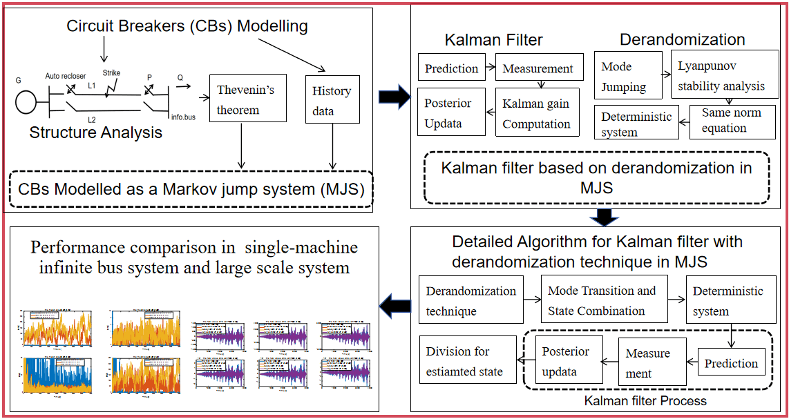
This study considers the state estimation problem of the circuit breakers (CBs), solving for random abrupt changes that occurred in power systems. With the abrupt changes randomly occurring, it is represented in a Markov chain, and then the CBs can be considered as a Markov jump system (MJS). In these MJSs, the transition probabilities are obtained from historical statistical data of the random abrupt changes when the faults occurred. Considering that the traditional Kalman filter (KF) frameworks based on MJS only depend on the subsystem of MJS, but neglect the stochastic jump between different subsystems. This study utilized the derandomization technique which transforms the stochastic MJS to a deterministic system to introduce the stochastic mode jumping in MJS, in which the state is still in the same norm, and the Lyapunov function is derived to show the stability condition of the systems, which proved that the transformed deterministic system is more conservative than the original MJS mathematically. After that, the Kalman filter algorithm is designed for estimating the state of the CBs depending on the transformed deterministic system. With the help of the Kalman filter, the estimation performance is derived by the recursive state estimation algorithm for the CBs. Furthermore, a single machine infinite-bus (SMIB) power system and a three-bus large scale system are proposed as practical examples to validate the effectiveness of the proposed algorithm.Graphic Abstract
Keywords
Over the past several decades, power systems have undergone substantial advancements and have garnered increasing attention from worldwide researchers. This growing interest is primarily attributed to the pivotal role that power systems play in a broad spectrum of industrial applications [1,2]. As modern society becomes increasingly reliant on electricity, ensuring the reliability, efficiency, and resilience of power systems has emerged as a critical engineering challenge. Power systems are inherently complex, characterized by nonlinear dynamic behavior and susceptibility to low-frequency oscillations. These oscillations are not merely theoretical constructs but constitute essential dynamic features that significantly influence the overall stability of the power grid. They typically arise from the interactions among various system components, including synchronous generators, transmission networks, and time-varying load dynamics. A comprehensive understanding and effective mitigation of such oscillatory behaviors are therefore indispensable for maintaining secure and stable system operation and preventing potential instability or cascading failures.
Efficient energy conversion and delivery across the different layers of the power infrastructure are crucial for minimizing transmission losses and ensuring a high-quality power supply to end-users. The integration of renewable energy sources introduces additional complexity due to their variable and intermittent nature, necessitating advanced control strategies and real-time balancing mechanisms to maintain equilibrium between supply and demand [3]. Furthermore, the concept of energy storage has gained increasing prominence in the context of modern power systems, offering viable solutions to address temporal mismatches between energy production and consumption. Effective energy management is also intrinsically linked to power quality, which encompasses parameters such as voltage sags, harmonics, and frequency deviations. Maintaining acceptable power quality levels is essential for safeguarding sensitive equipment and ensuring the reliable and uninterrupted operation of both residential and industrial loads.
Consequently, a holistic investigation of power systems must encompass not only dynamic behaviors such as low-frequency oscillations, but also broader aspects related to energy flow, conversion efficiency, and long-term sustainability. Understanding and optimizing the interplay between system dynamics and energy management strategies is vital for the development of resilient, intelligent, and adaptive power grids capable of meeting the evolving energy demands of future societies. Neglecting these oscillations can result in severe consequences. It may compromise the stability of the entire power system, leading to increased transmission losses and reduced transmission line capacities. These issues result in higher operational costs and diminished system efficiency. Moreover, the quality of power supplied to end-users can be significantly degraded, affecting sensitive electronic equipment and industrial processes. Consequently, addressing and mitigating these oscillations is essential for ensuring reliable and high-quality power delivery [4]. In recent years, the power area has introduced several novel techniques, such as the power system stabilizers (PSSs) [5], the high voltage direct current (HVDC) [6] and the static voltage condenser (SVC) [7], which decrease the influence of the oscillations. Throughout the techniques mentioned above, the PSSs is one of the most efficient and commonly used methods in recent years according to the conventional structure in the practical industrial field [8,9]. Even if nonlinear behavior occurred in the power system, the PSSs is a traditional control technique which is designed depending on the linearized power system model in assorted working conditions [10].
Considering that the abrupt changes usually occurred in the actual power system, which is one of the key difficulties, there are many reasons that result in such a phenomenon, for example, component repairs [11], subsystem connection changes [12] and environmental disturbance exist [13]. To solve such difficulty, the power system treats these abrupt changes as a Markov chain [14–16], in which modes may jump to each other stochastically within a finite set at any time and there is no relationship between the stochastic jumping at different times. In general, such a class of systems with abrupt changes obeying a Markov chain is represented as a Markov jump system (MJS) commonly, and the finite modes are the subsystems in MJS. In the last decade, numerous researchers have focused on the analysis of MJSs, such as Kuppusamy et al., who studied the asynchronous controller to solve the stabilization problem of power systems with random abrupt changes in 2021 [16]. In 2024, Bahmani utilized a non-stationary discrete Markov model to provide a precise and valuable understanding of the constantly evolving and time-dependent nature of the power network [14].
Tracking the state of the power system makes great sense because the evolution of the power system will be determined clearly, and a certain controller can be activated. Kalman filter (KF) is one of the most common state estimation technique, which track the state by weighted combining the model evaluation and the measurement. However, the system modes are unable to be derived online with the stochastic jumping among different subsystems. Therefore, there are some difficulties in applying the Kalman filter algorithm to the MJSs. In this scenario, Borisov et al. devoted themselves to the optimal state filtering of the finite-state Markov jump processes with given indirect continuous-time observations corrupted by Wiener noise in 2020 [17]. Zhang et al. designed a mode based Kalman filter for the MJSs with time correlated mode mismatch errors in 2021 [18]. In 2023, Costa et al. considered the finite horizon filtering problem of discrete-time Markov jump systems (MJS) satisfying some general nonlinear conditions [19].
However, most of the existing results are based on individual subsystems of the Markovian Jump System (MJS), while neglecting the stochastic transitions among different subsystems. In other words, the inherent randomness in mode jumping within MJSs is not adequately considered, which constitutes a significant limitation of these approaches, especially when applied to realistic MJS models. Generally, the Kalman filter (KF) framework based on subsystems of MJS requires prior knowledge of the current system mode before the recursive estimation process can be carried out. However, acquiring the exact mode information in practical MJSs is often either unavailable or computationally expensive, which poses a major challenge in the design of Kalman filters for such systems. To address this issue and develop an effective Kalman filtering algorithm for MJSs with stochastic mode transitions, a derandomization technique has been proposed [20,21]. This technique transforms the stochastic MJS into an equivalent deterministic system, in which the random mode transitions are embedded as part of the system dynamics. As a result, the Kalman filter can be directly applied to the transformed system, where the state maintains the same norm as that of the original MJS. This ensures that the estimation obtained from the transformed system is equivalent to that of the original MJS.
Moreover, the requirement for real-time mode determination in MJSs is effectively eliminated in the transformed deterministic framework. The stochastic mode jumping behavior is inherently incorporated into the estimation process through the system transformation. In addition, the performance of the Kalman filter is evaluated, demonstrating the effectiveness of the proposed approach and contributing to the advancement of Kalman filter design for MJSs.
The rest of this paper is organized as follows: In Section 2, the descriptions of power systems are provided, which are modeled in MJS and the derandomization technique is given, which transforms the discrete-time MJS to a deterministic system. In Section 3, the Kalman filter design based on the transformed deterministic system is presented. Then, the practical application of circuit breakers (CBs) exhibits the validity of the proposed technique in Section 4. The conclusion is given in Section 5.
Notations:
In this section, the detail of the Circuit Breakers working process is shown in Fig. 1 at first. In this figure, no matter the transient strikes or permanent faults occur online, the circuit breakers (CBs) isolate the line immediately to protect the whole power system network. After a while, the CBs will attempt to auto-reclose, which tests whether the power system would work normally. In common sense, the transient fault occurred due to the strike will end in several seconds. However, if the faults are unable to elapse transiently, which means the permanent fault occurs on line, then emergency repairs are needed.
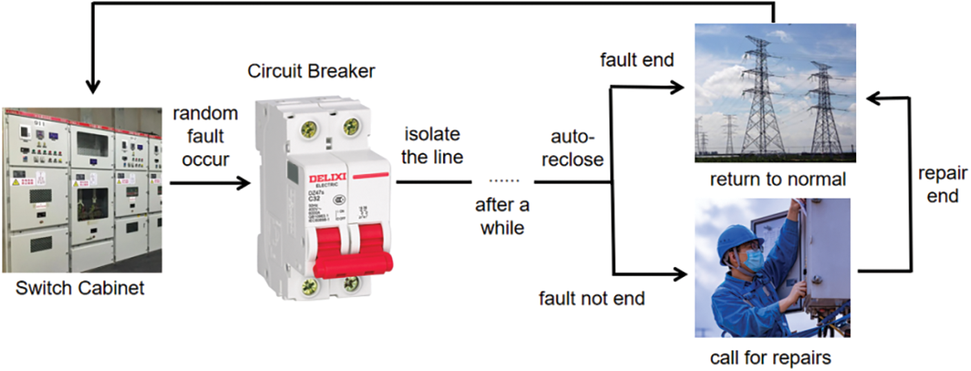
Figure 1: Working process of circuit breakers
To show the practical circuit breaker in a switch cabinet in a power system much more clearly, the structure can be modeled as a single-machine connected to an infinite-bus (SMIB) with typical circuit components [22]. The machine is equipped with a thyristor exciter and the SMIB is represented by the Thevenin equivalent of a large power system network. Considering that simultaneous faults occurring on both lines are extremely rare in practice, this paper assumed that only one line has malfunctioned probably, in which the faults, usually known as the stream of lightning strikes at random time instants, are setting on line in this study. The structure of the SMIB subject to random faults is provided in Fig. 2.
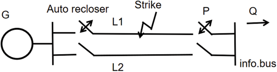
Figure 2: The structure of SMIB subject to random faults
With the relationship between the variables analyzed based on Thevenin’s theorem, the nonlinear system model is proposed by the following differential equations [23].
where
Then we set the state vector as
which can be simply written as
As mentioned previously, the Markov chain is utilized to analyze the random abrupt topology changes of the subsystem structure in power systems. Considering that the random abrupt changes and the shift operator of Eq. (2) can be discretized as a discrete-time Markov jump system (MJS), and the parameters of the MJS are identified depending on the mechanistic models and historical data by the least squares method. Then the MJS state evaluation model is written as follows:
where
Considering that the system is modeled in MJS, the transition probability
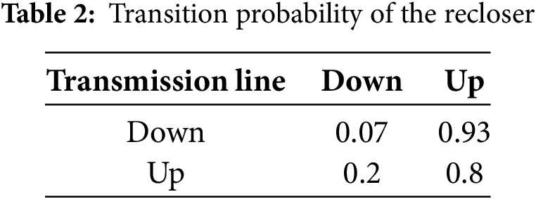
Then the mode transition of up and down modes and the transition probability are proposed in Fig. 3.
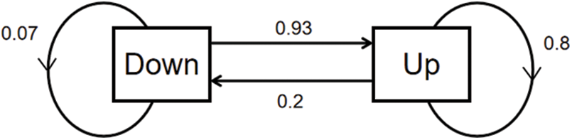
Figure 3: Transition of the MJSs modes depending on the line failure
Meanwhile, we consider the measurements of the MJSs (3) as follows:
where
The problem proposed in this paper can be formulated as estimating the discrete power system modeled as Eqs. (3) and (4) recursively. In MJSs, the stochastic mode jumping is the key problem for the recursive state estimation process. Considering the transition probability in MJSs, one of the most widely accepted ideas is weighting the next moment mode based on the transition probability according to the mode in the current moment. Depending on this idea, the probable mean of the state is derived based on the weighted mode prediction. Considering that the weighted idea is able to transform the stochastic MJS to a deterministic one, this idea can be formulated as a derandomization technique. Therefore, to establish the recursive state estimation based on the power system with a stochastic jumping problem, the derandomization technique is proposed in the following.
Firstly, a Dirac function
Then define:
where
Combining Eqs. (3) and (5) and considering the definition of the Dirac function
Then, define the extended state vector and the extended noise vector as:
where
Till Eq. (8), the discrete MJS (3) with stochastic mode jumping is transformed to a deterministic system in Eq. (8), in which the state only evolves depending on moment
Remark 1: With the help of the derandomization technique, the CBs modeled in MJS can be transformed to single mode system, and the extended state vector in the transformed system has the same expectation as the original MJS, the corresponding parameter of expectation is the mean and the state estimation is mean value estimation.
For better understanding, the Lyapunov function of these transformed systems based on the derandomization technique and the original MJS is proposed to verify the system stability as follows:
Lyapunov stability criterion for MJS: There exists a group of positive definite symmetric matrix
If all the inequalities above are listed in the inequality matrix, it can be formulated as:
Considering that all the diagonal elements in the above inequality matrix are
Considering that the transition probability elements
As commonly known that all the elements in the transition probability matrix
After combining the multiplication of diagonal matrix
We notice that all
Therefore, the stability inequality is proposed as:
Above all, the Lyapunov function of both the original MJS (3) and the transformed deterministic system (8) is provided. The stability constraints in (8) are more conservative than (3), which implies that when the transformed deterministic system (8) is stable, the MJS (3) is stable as well, according to the Lyapunov function. This verifies the statement that the state has the same norm between the MJS (3) and the transformed deterministic system (8) after the utilization of the derandomization technique.
After the deterministic system is achieved, the Kalman filter is designed in the next section.
In this section, the recursive state estimation based on the Kalman filter algorithm is derived depending on the transformed deterministic system derived in Eq. (13).
Then the explicit expression of the deterministic system is given as:
where
where
Then the Kalman filter based on the transformed deterministic system begins the recursive algorithm with the one step prior state prediction
where
Then the Kalman filter gain can be computed as follows:
With the Kalman filter gain derived, the posterior state estimation is given in the following equation:
Meanwhile, the posterior of the covariance is:
Above all, the recursive state estimation result based on the MJS model of CBs is proposed as Algorithm 1 [20] follows:
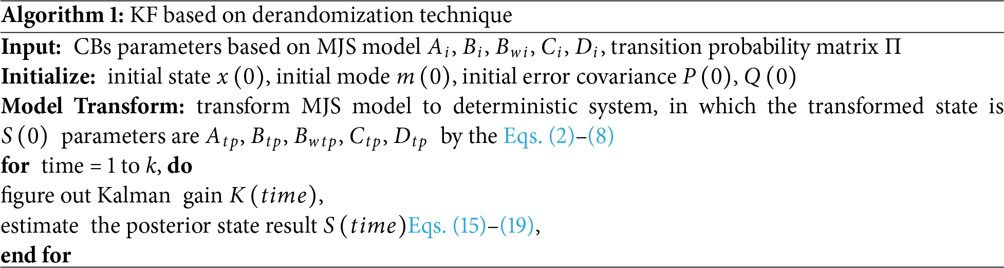
Considering the transformed large-scale system, the key difference is the multiplicatively increasing dimension resulting from the Kronecker product, which has heavier computation complexity in the recursive estimation process, especially figuring out the Kalman gain with the high dimension matrix inverse in Eq. (17).
After the algorithm’s proceedings are provided, the estimation performance of the result is shown by the root mean square error (RMSE) as follows:
According to Eqs. (11)–(15), the optimal posterior recursive estimation result
Considering the system transformation process, it is easy to understand that the transformed state
Corollary 1 (Expectation method): Based on the MJS (3), the related system parameters are presented as
Corollary 2 (Subsystem based method): Based on the MJS (3), the parameters of the recursive state estimation methods are based on the subsystem parameters
Remark 2: Compared to the derandomization technique, Corollary 1 and 2 using the expectation of the matrix
For better understanding, a theoretical comparison table of the proposed method and existing techniques is provided as follows in Table 3:
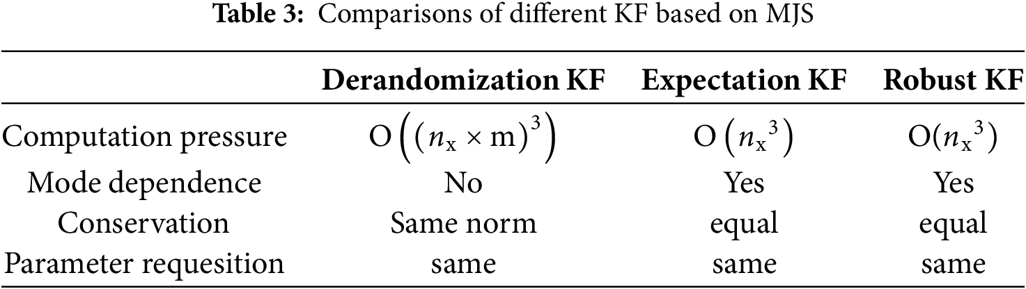
With the existing study of the recursive estimation of MJS given in corollary 1 and 2, the comparison between the algorithms mentioned above is revealed by the performance index RMSE given in Section 4.
4 Experimental Validation and Discussion
In this section, the performance of the Kalman filter algorithm incorporating a derandomization technique is demonstrated through the CBs examples in a practical power system. A two mode, one bus single system and a three-bus large scale system are provided to demonstrate the proposed KF based on derandomization technique. This simulation highlights the effectiveness and superiority of the proposed approach.
All the power system models are implemented using Simulink in MATLAB R2022a. The two mode one bus system modeled in MJS is divided by the mode indication signal, as illustrated in Fig. 4. Then the state is proposed from the scope. The sampling interval is 1 s for each sample.
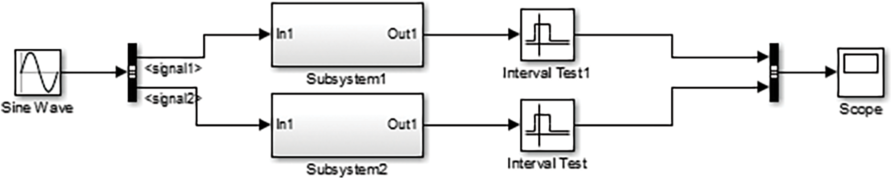
Figure 4: Simulink figure of the power system
In the following, the on-off switching behavior of circuit breakers (CBs) during line faults in a Markovian Jump System (MJS) with two modes, the occurrence of transient fault and permanent fault, is parameterized as follows [23]. All the parameters are derived from the historical statistical data according to the Thevenin’s theorem in Eqs. (1)–(4) from the reference. The parameters of the considered system are represented as follows: the synchronous motor machine parameters:
As mentioned before, the goal of this paper is to design a recursive state estimation algorithm based on the derandomization technique. In this practical example, the Markov jump process has two modes and the transition probability matrix is given by
Fig. 5 illustrates the stochastic transitions between the up and down modes exhibited by the system. To further elucidate the system’s behavior, Fig. 6 presents the open-loop variations of the four state variables during these mode transitions.
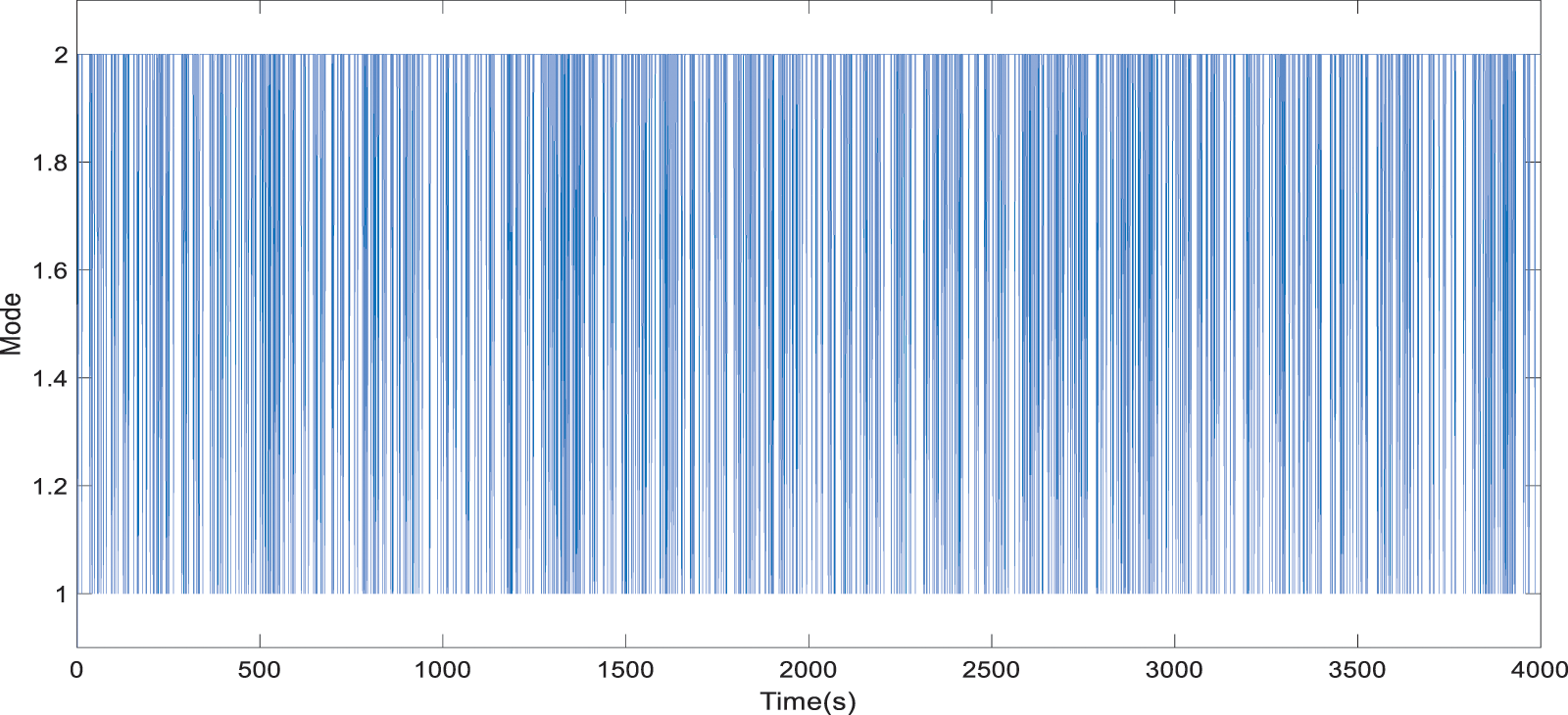
Figure 5: Mode transition between two modes
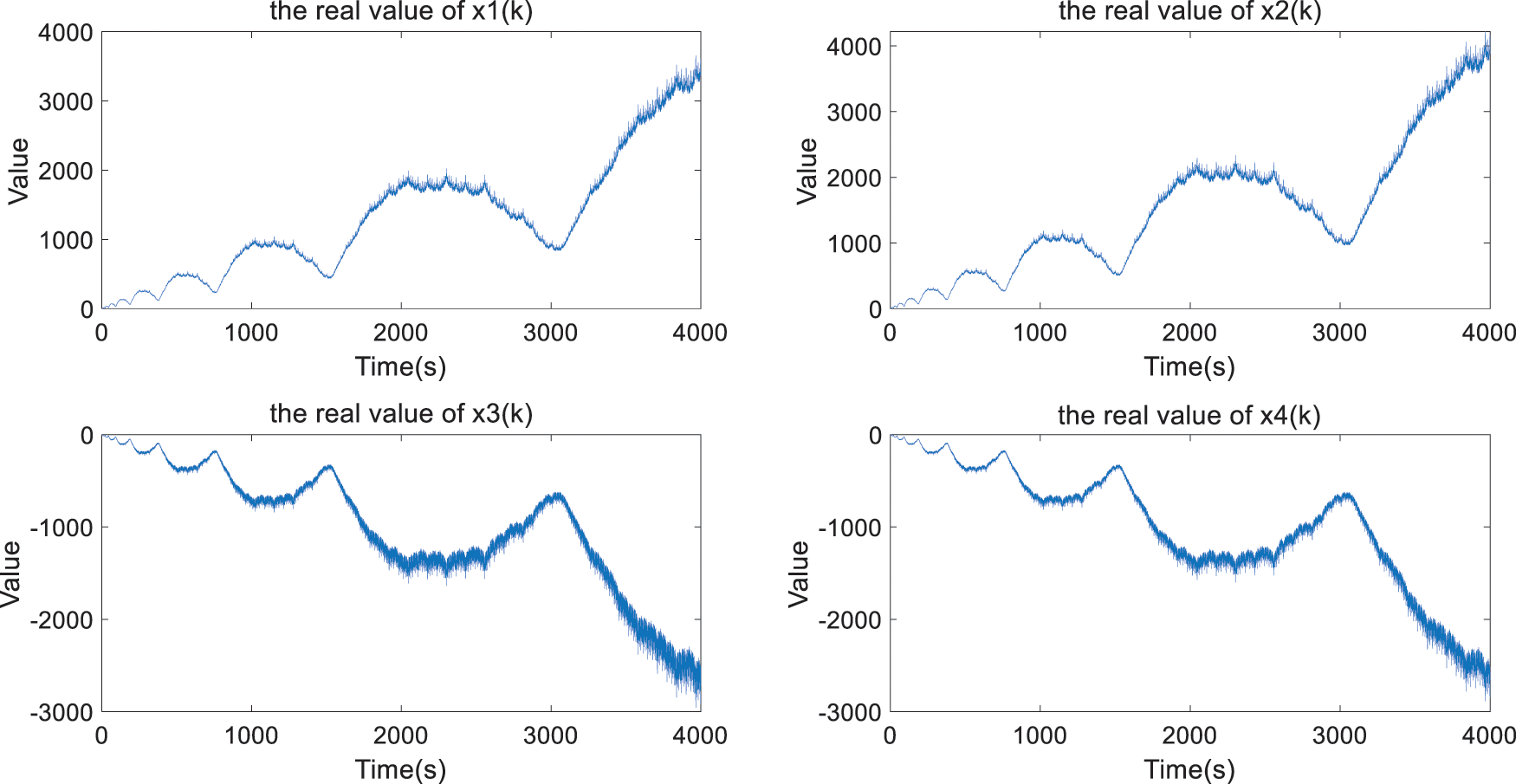
Figure 6: Open-loop state variation
To stabilize this open-loop system, a conservative solution based on feedback control is given by the linear matrix inequalities (LMI). Then the Kalman gain based on the stable system is given as follows:
The Kalman gain of the proposed method is based on the extended batch of states, and it can be divided into two Kalman gains depending on each subsystem that:
With the mathematical proof that the transformed deterministic system is a more conservative system than the original MJS in the previous section, the Kalman gain is available for the two modes, the transient fault and the permanent fault. Furthermore, the stochastic mode switching is considered as well by such a technique.
Fig. 7 shows the estimation results and the real value of the recursive state estimation algorithm. To show the estimation performance, the RMSEs derived from Eq. (15) are given in Fig. 8. The stochastic mode transition of the Markov chain (
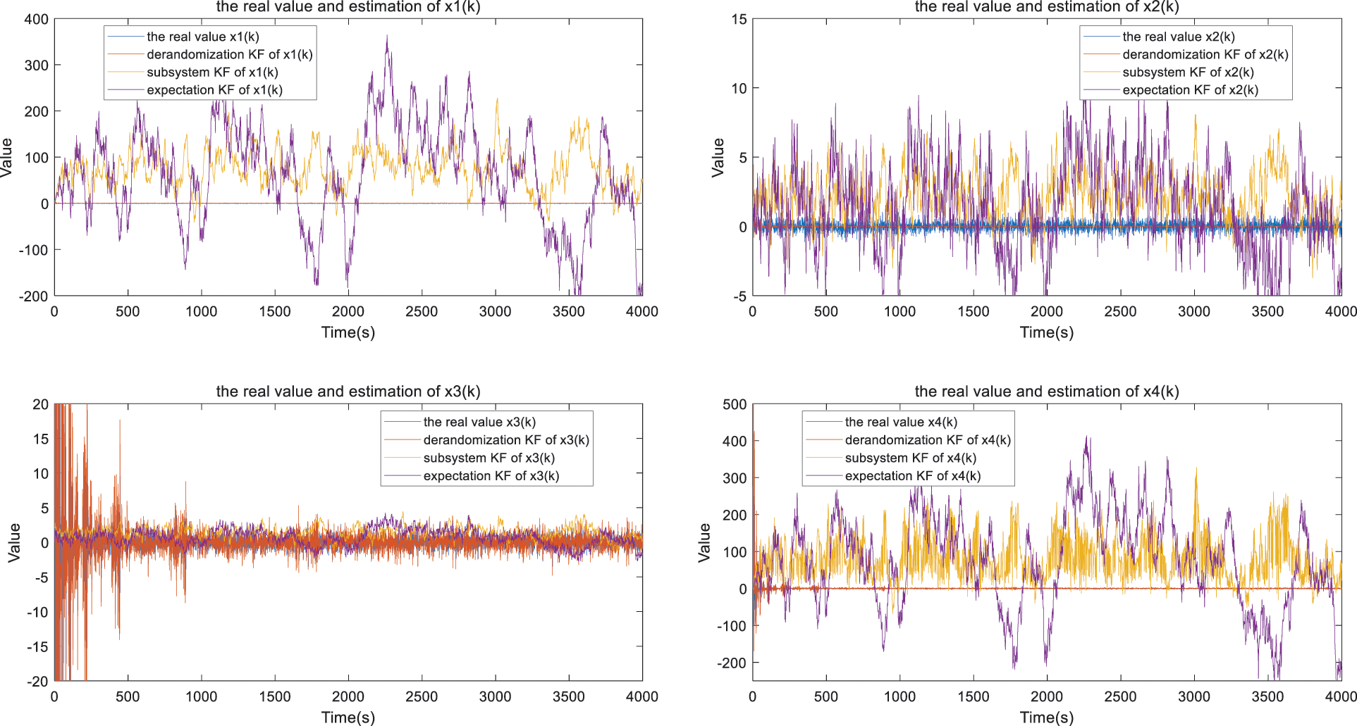
Figure 7: The estimation result and the real value of each state component
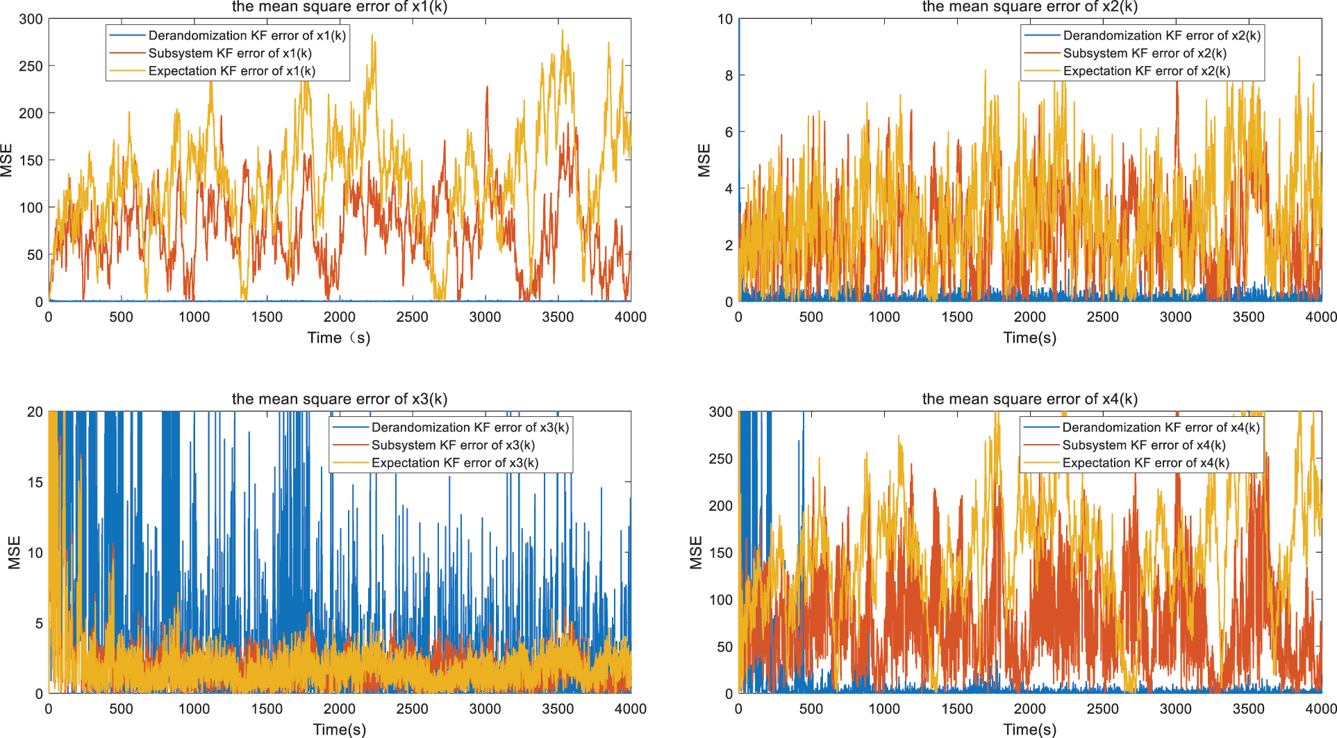
Figure 8: The RMSE of each state component in different KF algorithms
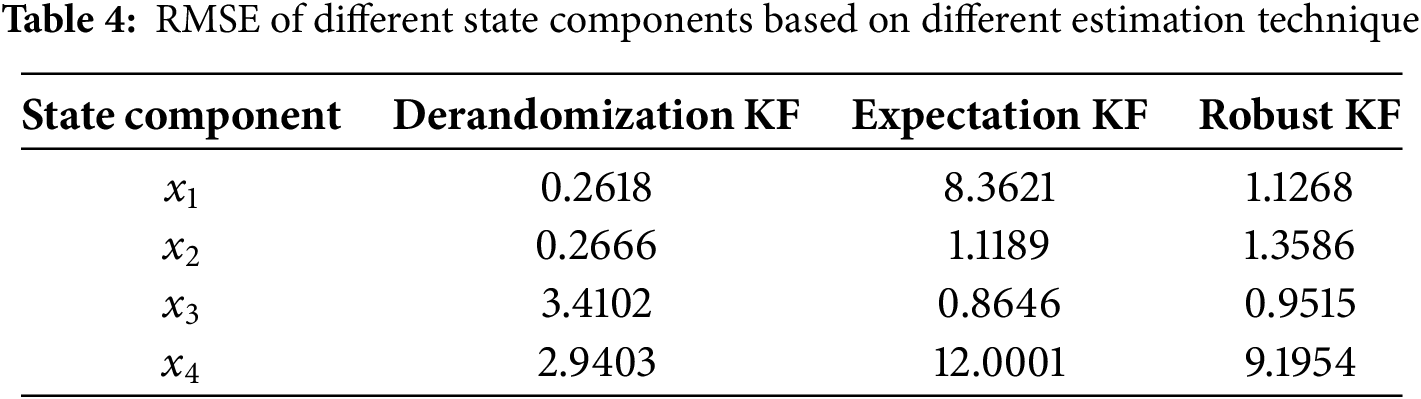
From the simulation results presented above, it is evident that the recursive state estimation algorithm for Markovian Jump Systems (MJSs) in power systems performs effectively when the derandomization technique is applied. This approach explicitly accounts for the stochastic mode transitions during the estimation process. By incorporating the randomness of mode jumping in the MJS modeling of circuit breakers (CBs), the proposed method achieves significantly lower root mean square error (RMSE) in state estimation compared to the expectation-based method in Corollary 1 and the robust method in Corollary 2.
Fig. 7 illustrates the true system states alongside the estimated values, while Fig. 8 presents the RMSEs of the aforementioned methods discussed in the previous section. To further demonstrate the estimation performance, Table 1 summarizes the RMSE values obtained from the estimation process. Compared to the existing results studied in 2023 [19], it is obvious that the derandomization technique has transformed the stochastic mode jumping in MJS to a deterministic system, which has the same norm as the original MJS. The existing KF framework mostly estimates the state based on each subsystem or the expectation of the weighted modes. Then, the MJS-KF based on the subsystem has not introduced the transition probability information. Especially, the transition probability affects the stability of the MJS, which is clearly proved in the Lyapunov stability constraints. Else, the estimation error of KF based on the expected weighted modes of MJS is obviously larger than the proposed technique due to the hybrid weighted mode information introduced. Besides, all these existing KF frameworks have the constraint that the current mode should be known. Nevertheless, the proposed MJS-KF based on the derandomization technique can begin the estimation process without the need for known current mode information.
Additionally, to compare this proposed method with recent advancements in MJS-based Kalman filtering, there is an expanded discussion. In [24], it analyzes the convergence characteristics of the factorial Kalman filter, which ensures that the Kalman gain converges at t → ∞. Specifically, it provides sufficient convergence conditions for Kalman gain, but it is not suitable for the state estimation problem of the circuit breakers (CBs) solving random abrupt changes that occur in power systems. In [25], Bayesian deep learning and Kalman net are integrated to quantify uncertainty without additional domain knowledge by sampling prediction error covariance. However, it relies on many training data and GPU calculations, and its real-time performance is poor. The deterministic transformation in this paper only needs the historical transition probability, and the calculation time in the SMIB system is less, which is more suitable for online estimation of the power system. Reference [26] proposes an improved maximum correlation entropy Kalman filter to enhance the robustness to non-Gaussian noise (such as impulsive noise) by introducing a weighted factor cost function. However, the method in [26] needs to manually adjust the kernel width parameter, which limits its generalization in the power system catastrophe scenario. In this paper, the solution of randomization depends on the historical statistical noise model. In the CB Gaussian noise scene studied in this paper, RMSE is equivalent to IMCKF, but the implementation is simpler. Furthermore, the Kalman filter Gaussian mixture model is presented in [27]. The Gaussian mixture model is used to approximate the fuzzy TDOA measurement and improve the accuracy of multi satellite positioning. However, the computational complexity increases exponentially with the number of mixed components, which makes it difficult to extend to large power grids. In this paper, the solution randomization compresses the multi-modal MJS into a single-mode system. In SMIB, only a single Kalman filter is needed, and the memory consumption is reduced.
Overall, the necessity and superiority of the derandomized MJS-based Kalman filter are clearly demonstrated based on the results shown in Figs. 7 and 8 and Tables 3 and 4, particularly when compared with existing Kalman filter algorithms designed for MJSs.
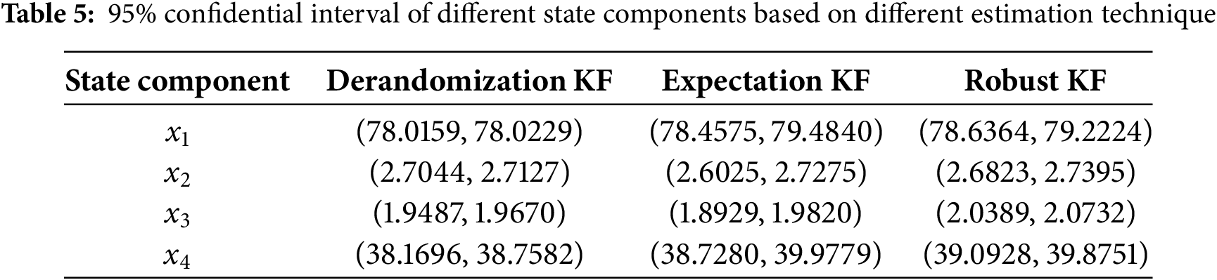
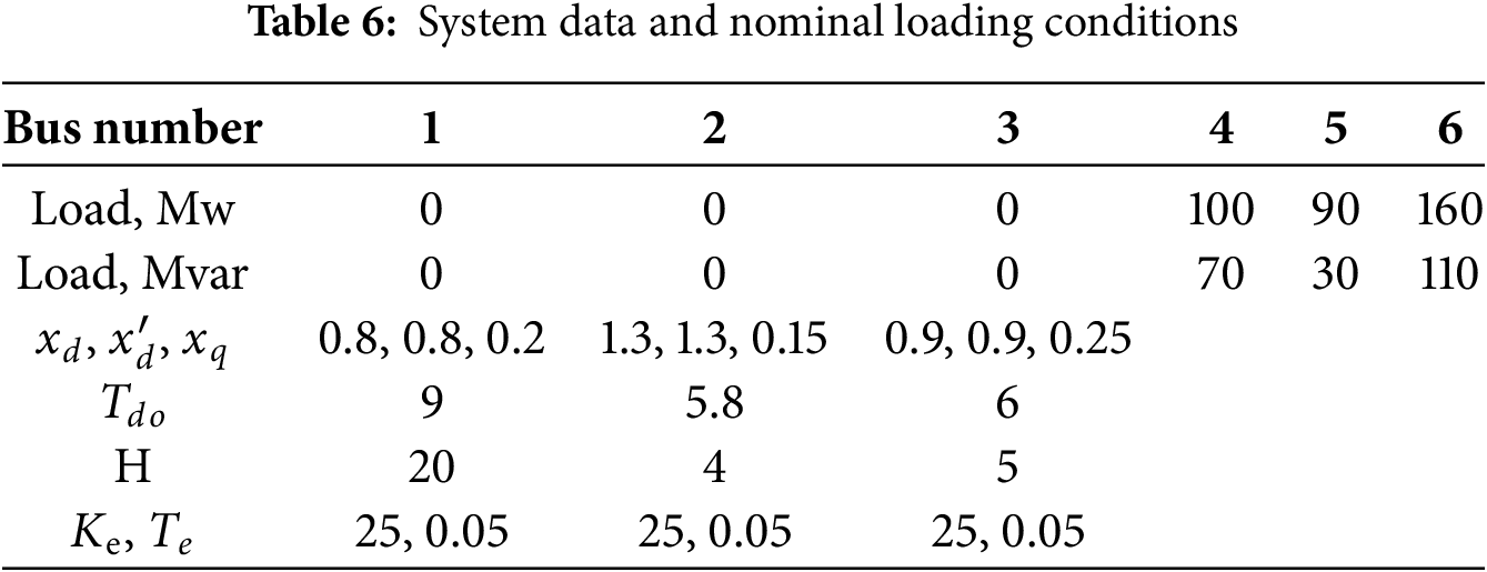
For better verification, a multi-machine case with 6-bus and 3-machine in the system is provided, and the structure is shown in Fig. 9 [22]. In this system, random faults occurred in lines 1–4 and 1–5, which are modeled as three subsystems in MJS. As listed in the reference, the critical parameters are proposed in Table 6.
Figure 9: 6-buses and 3-machine system
Then the MJS model parameters can be formulated as:
The transition probability matrix of this large-scale system is
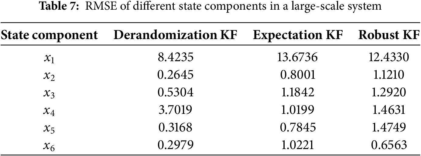
The estimation result of each state component is provided in Fig. 10. In this figure, it can be found that periodic oscillations occurred in the state components, which is more complicated than that in the SMIB instance. Then the estimation result of the KF framework based on the derandomization technique, the subsystems and weighted expectation are provided. Obviously, even the absolute value of the state component varies in a large range. The proposed technique can help the KF framework track the real state as well, which clearly exhibits the effectiveness and priority of the proposed technique. For better understanding, Table 7 provides the RMSE of the estimation result in the large-scale power system. From the estimation result figure and the error table, the estimation tracks the real state, but the estimation error is different. Mostly, the state components have the lowest estimation error except x4 with the help of KF based on the derandomization technique.
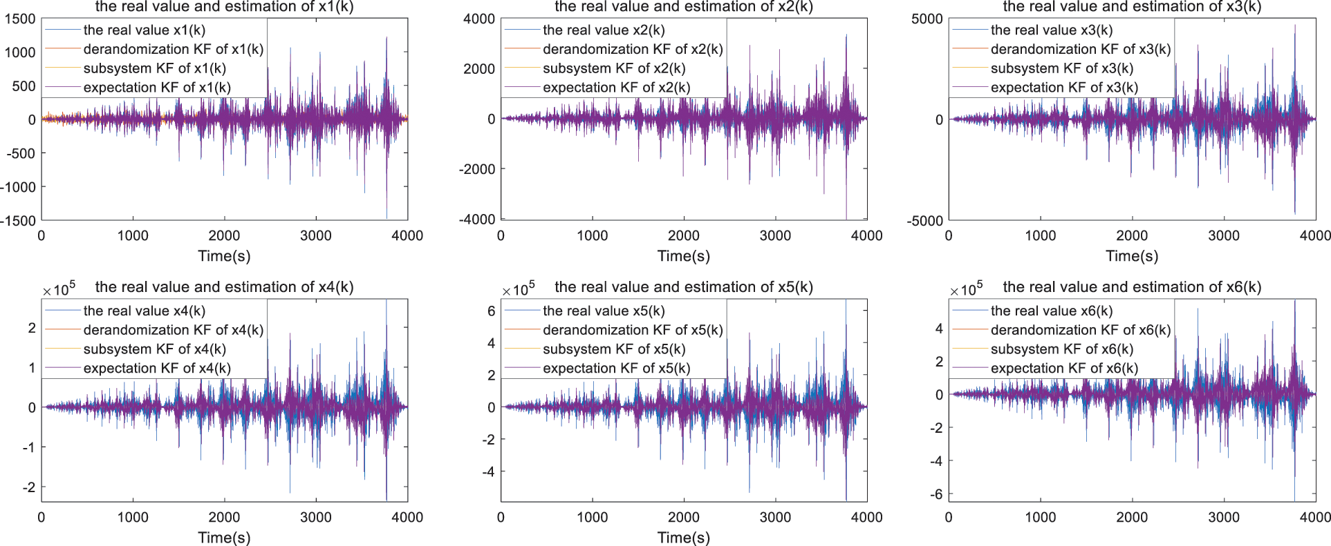
Figure 10: The estimation result and the real value of each state component in a large-scale system
From the above simulation results, it can be found that this proposed method has the potential to be applied in the multi-machine cases, like 6-bus and 3-machine. However, it must also be admitted that when this method is applied to large-scale power grids, there will be a curse of dimensionality, that is, by randomizing the m-mode MJS into a single mode system, but the state dimension will rapidly expand, requiring high solving ability. It should be noted that by aggregating equivalent circuits of large-scale power grids, the dimension of the state matrix can be reduced, so this method still has certain generalizability.
This paper proposes a recursive state estimation algorithm based on derandomization for Markov Jump Systems (MJSs) in power system applications. The power system with random abrupt changes is first modeled as an MJS, considering stochastic mode transitions governed by a Markov process. Using derandomization, the MJS is transformed into an equivalent deterministic system while preserving the state norm. A recursive estimation algorithm is then developed based on this transformed system. For comparison, existing Kalman filtering methods for MJSs are also revealed, where mode-dependent parameters are approximated as well. In the case of circuit breakers (CBs), the proposed method converts the MJS model into a single-mode system, and the Kalman filter is applied to estimate the state while accounting for stochastic switching among subsystems. Simulation results on a CB model demonstrate the effectiveness and superiority of the proposed approach over existing algorithms. Furthermore, parameter uncertainties caused by component failures are common in real-world power systems, suggesting that future work should focus on recursive state estimation under unknown or time-varying system parameters to enhance robustness in practical energy systems. Future research may attempt to develop recursive state estimation algorithms capable of handling uncertain parameters under fault conditions, thereby improving the robustness and practical applicability of estimation techniques in complex power systems. Such advancements are essential for enhancing the observability and resilience of smart grids, particularly in the presence of high renewable energy penetration and dynamic load behaviors.
Acknowledgement: Not applicable.
Funding Statement: The authors received no specific funding for this study.
Author Contributions: The authors confirm contribution to the paper as follows: Conceptualization, Quan Li and Ziheng Zhou; methodology, Ziheng Zhou; software, Ziheng Zhou; validation, Ziheng Zhou; formal analysis, Ziheng Zhou; investigation, Quan Li; resources, Quan Li; data curation, Quan Li; writing—original draft preparation, Ziheng Zhou; writing—review and editing, Ziheng Zhou; visualization, Quan Li; supervision, Quan Li; project administration, Quan Li; funding acquisition, Quan Li. All authors reviewed the results and approved the final version of the manuscript.
Availability of Data and Materials: The data that support the findings of this study are available from the Corresponding Author, Quan Li, upon reasonable request.
Ethics Approval: Not applicable.
Conflicts of Interest: The authors declare no conflicts of interest to report regarding the present study.
References
1. Anderson PM, Fouad AA. Power system control and stability. Hoboken, NJ, USA: John Wiley & Sons, Inc.; 2008. [Google Scholar]
2. Rafique Z, Khalid HM, Muyeen SM, Kamwa I. Bibliographic review on power system oscillations damping: an era of conventional grids and renewable energy integration. Int J Electr Power Energy Syst. 2022;136(3):107556. doi:10.1016/j.ijepes.2021.107556. [Google Scholar] [CrossRef]
3. Khalid HM, Flitti F, Mahmoud MS, Hamdan MM, Muyeen SM, Dong ZY. Wide area monitoring system operations in modern power grids: a Median regression function-based state estimation approach towards cyber attacks. Sustain Energy Grids Netw. 2023;34(2):101009. doi:10.1016/j.segan.2023.101009. [Google Scholar] [CrossRef]
4. Khalid HM, Qasaymeh MM, Muyeen SM, El Moursi MS, Foley AM, Sweidan TO, et al. WAMS operations in power grids: a track fusion-based mixture density estimation-driven grid resilient approach toward cyberattacks. IEEE Syst J. 2023;17(3):3950–61. doi:10.1109/JSYST.2023.3285492. [Google Scholar] [CrossRef]
5. Nocoń A, Paszek S. A comprehensive review of power system stabilizers. Energies. 2023;16(4):1945. doi:10.3390/en16041945. [Google Scholar] [CrossRef]
6. India SU, Kumar A, Akbar Hussain DM, Denmark AU. HVDC (high voltage direct current) transmission system: a review paper. Gyancity J Eng Technol. 2018;4(2):1–10. doi:10.21058/gjet.2018.42001. [Google Scholar] [CrossRef]
7. Mahmud SU, Nahid-Al-Masood. Performance comparison between synchronous condenser and static VAR compensator to improve system strength in a wind dominated power grid. In: 2020 11th International Conference on Electrical and Computer Engineering (ICECE); 2020 Dec 17–19; Dhaka, Bangladesh. doi:10.1109/icece51571.2020.9393153. [Google Scholar] [CrossRef]
8. Hatziargyriou N, Milanovic J, Rahmann C, Ajjarapu V, Canizares C, Erlich I, et al. Definition and classification of power system stability-revisited & extended. IEEE Trans Power Syst. 2021;36(4):3271–81. doi:10.1109/TPWRS.2020.3041774. [Google Scholar] [CrossRef]
9. Zhang G, Hu W, Cao D, Huang Q, Yi J, Chen Z, et al. Deep reinforcement learning-based approach for proportional resonance power system stabilizer to prevent ultra-low-frequency oscillations. IEEE Trans Smart Grid. 2020;11(6):5260–72. doi:10.1109/TSG.2020.2997790. [Google Scholar] [CrossRef]
10. Kim JJ, Park JH. A novel structure of a power system stabilizer for microgrids. Energies. 2021;14(4):905. doi:10.3390/en14040905. [Google Scholar] [CrossRef]
11. Peyghami S, Blaabjerg F, Palensky P. Incorporating power electronic converters reliability into modern power system reliability analysis. IEEE J Emerg Sel Top Power Electron. 2021;9(2):1668–81. doi:10.1109/jestpe.2020.2967216. [Google Scholar] [CrossRef]
12. Afzal S, Mokhlis H, Illias HA, Mansor NN, Shareef H. State-of-the-art review on power system resilience and assessment techniques. IET Generation Trans Dist. 2020;14(25):6107–21. doi:10.1049/iet-gtd.2020.0531. [Google Scholar] [CrossRef]
13. Bhusal N, Abdelmalak M, Kamruzzaman M, Benidris M. Power system resilience: current practices, challenges, and future directions. IEEE Access. 2020;8:18064–86. doi:10.1109/access.2020.2968586. [Google Scholar] [CrossRef]
14. Bahmani MH, Esmaeili Shayan M, Fioriti D. Assessing electric vehicles behavior in power networks: a non-stationary discrete Markov chain approach. Electr Power Syst Res. 2024;229(1):110106. doi:10.1016/j.epsr.2023.110106. [Google Scholar] [CrossRef]
15. Han X, Wei Z, Hong Z, Zhao S. Ordered charge control considering the uncertainty of charging load of electric vehicles based on Markov chain. Renew Energy. 2020;161(2):419–34. doi:10.1016/j.renene.2020.07.013. [Google Scholar] [CrossRef]
16. Kuppusamy S, Joo YH, Kim HS. Asynchronous control for discrete-time hidden Markov jump power systems. IEEE Trans Cybern. 2021;52(9):9943–8. doi:10.1109/tcyb.2021.3062672. [Google Scholar] [PubMed] [CrossRef]
17. Borisov A, Sokolov I. Optimal filtering of Markov jump processes given observations with state-dependent noises: exact solution and stable numerical schemes. Mathematics. 2020;8(4):506. doi:10.3390/math8040506. [Google Scholar] [CrossRef]
18. Zhang W, Natarajan B. On the performance of Kalman filter for Markov jump linear systems with mode mismatch. Circuits Syst Signal Process. 2021;40(4):1720–42. doi:10.1007/s00034-020-01545-0. [Google Scholar] [CrossRef]
19. Costa OLV, de Oliveira AM. Filtering for nonlinear and linear Markov jump systems. IEEE Trans Autom Control. 2024;69(5):3309–16. doi:10.1109/TAC.2023.3322379. [Google Scholar] [CrossRef]
20. Wan H, Karimi HR, Luan X, Liu F. A self-triggered control scheme for Markov jump systems under multiple range performance restrictions. IFAC-PapersOnLine. 2020;53(2):2783–8. doi:10.1016/j.ifacol.2020.12.938. [Google Scholar] [CrossRef]
21. Allagui A, Elwakil AS. On the theory and application of the fractional-order Dirac-delta function. IEEE Trans Circuits Syst II Express Briefs. 2024;71(3):1461–5. doi:10.1109/TCSII.2023.3324702. [Google Scholar] [CrossRef]
22. Soliman H, Shafiq M. Robust stabilisation of power systems with random abrupt changes. IET Generation Trans Dist. 2015;9(15):2159–66. doi:10.1049/iet-gtd.2014.1111. [Google Scholar] [CrossRef]
23. Kaviarasan B, Sakthivel R, Kwon OM. Robust fault-tolerant control for power systems against mixed actuator failures. Nonlinear Anal Hybrid Syst. 2016;22:249–61. doi:10.1016/j.nahs.2016.05.003. [Google Scholar] [CrossRef]
24. Qi C, Li Y, Bao J, Zhu M. Convergence analysis of the factorial Kalman filter. IEEE Signal Process Lett. 2025;32:2249–53. doi:10.1109/lsp.2025.3567424. [Google Scholar] [CrossRef]
25. Dahan Y, Revach G, Dunik J, Shlezinger N. Bayesian KalmanNet: quantifying uncertainty in deep learning augmented Kalman filter. IEEE Trans Signal Process. 2025;73:2558–73. doi:10.1109/tsp.2025.3581703. [Google Scholar] [CrossRef]
26. Zhao X, Mu D, Gao Z, Zhang J, Li G. Stochastic stability of the improved maximum correntropy Kalman filter against non-Gaussian noises. Int J Control Autom Syst. 2024;22(3):731–43. doi:10.1007/s12555-021-1119-4. [Google Scholar] [CrossRef]
27. Zhang Y, Wang H, Zheng J, Hua L, Zhang R, Xie J. Localization and ambiguity resolution algorithm for time-difference fusion of three satellites based on observation filtering. Sci Rep. 2025;15(1):26060. doi:10.1038/s41598-025-10236-2. [Google Scholar] [PubMed] [CrossRef]
Cite This Article
 Copyright © 2025 The Author(s). Published by Tech Science Press.
This work is licensed under a Creative Commons Attribution 4.0 International License , which permits unrestricted use, distribution, and reproduction in any medium, provided the original work is properly cited.
 Downloads
 Citation Tools