Single-Phase Grounding Fault Identification in Distribution Networks with Distributed Generation Considering Class Imbalance across Different Network Topologies

1  Introduction

1.1 Research Motivation and Background

In power systems, distribution network faults account for more than 85% of the total number of faults, of which the proportion of single-phase ground faults is more than 80%. The complexity and variability of the distribution network structure and the flexibility of the operation mode, as well as the large-scale access of DERs and the emergence of new distribution network structures, make the fault signals show a high degree of diversity and nonlinear complexity, which greatly increase the difficulty of fault identification in the distribution network [1,2]. After a fault occurs, whether it is possible to quickly and accurately determine the fault type and accordingly take timely and effective treatment measures to minimize the scope and time of the fault impact, which is the key link to ensure the reliable operation of the distribution system.

1.2 Literature Review

Currently, the analysis for single-phase ground faults mainly focuses on the electrical feature extraction and identification of post-fault data. Researchers usually collect electrical quantity information, such as zero sequence current/voltage from specified measurement points of distribution lines, and complete the diagnosis of fault types through signal processing and pattern recognition methods.

Among the signal processing and feature extraction methods are: using S-transform combined with neural network for classification [3,4]; applying wavelet decomposition combined with principal component analysis (PCA) for key feature selection [5]; using Hilbert-Huang transform (HHT) to convert time-domain features into frequency-domain information [6]; and using VMD combined with CNN for fault detection and classification [7]. Although these methods are more mature, there are still limitations: the selection of wavelet basis function is dependent on experience and lacks adaptivity; the S transform is computationally intensive and limited in frequency resolution; FFT [8], as a global transform, lacks the ability of time-frequency localization, and it is difficult to capture time-varying characteristics of the signal.

In recent years, artificial intelligence techniques have been widely used in the electric power field [9–12]. For example, reference [13] combined wavelet analysis with XGBoost model to achieve fault detection in neutral ungrounded systems, while reference [14] utilized the K-nearest neighbor (KNN) algorithm to classify wavelet-based energy ratios, coefficient variances, and power as input features. Since Hinton et al. proposed unsupervised feature learning based on Restricted Boltzmann Machine (RBM) [15], deep learning has provided new ideas for single-phase ground fault diagnosis by virtue of its powerful automatic feature extraction capability. However, the “black box” nature of deep learning makes its working mechanism difficult to be understood intuitively. Notably, techniques such as gradient-weighted class activation mapping (Grad-CAM) [16] visualize the prediction process of the network by generating a heat map, which provides a powerful tool for understanding and analyzing the decision logic of the model, and helps to improve the interpretability of the model.

In addition, existing fault sample generation methods typically generate a typical but balanced set of fault samples by evenly distributing the samples according to parameters such as fault location, type, and transition resistance. However, the actual fault tripping records in the field show [17] that there is a serious category imbalance problem in the number of samples corresponding to different fault causes. Therefore, when studying the fault identification model, it is necessary to consider the characteristics of actual faults and their probability distributions, and construct a category-imbalanced fault sample set that conforms to the actual situation, in order to enhance the generalization performance and practical value of the model in actual complex scenarios.

1.3 Contributions and Chapter Arrangement

In order to solve the above problems, a single-phase grounding fault identification method for distribution network based on two-dimensional images was proposed, with the core adopting the CBAM-ResNet18 model. The main contributions include: analyzing the probability distribution characteristics of key parameters such as neutral grounding mode, fault cause, and fault phase angle in the actual distribution network, so as to construct a sample set of category imbalance faults that is more suitable for the actual field; converting the fault zero-sequence current waveform into a 2D image, and inputting it into the Convolutional Neural Network (CNN) model that integrates the Convolutional Block Attention Module (CBAM), which is capable of guiding the model to focus on the key spatial and temporal characteristics of the signal, and enhancing the feature extraction. The CBAM can guide the model to focus on the key spatial and temporal features of the signal and enhance the feature extraction capability. At the same time, the Grad-CAM technique is used to visualize the attention area of the model, verify the effectiveness of the attention mechanism, and improve the model interpretability; the model is trained with proportionally sampled zero-sequence current image samples, and the high-precision recognition performance of the model is verified by MATLAB/SIMULINK simulation data and field recording data. Further module ablation study and noise-augmented test are conducted to verify the contribution of the CBAM module and the robustness of the model under noise interference.

This paper is structured as follows: Section 2 analyses the unbalance problem of single-phase ground fault class in distribution networks. Section 3 proposes a single-phase ground fault identification method based on CBAM-CNN, detailing the CBAM module, ResNet18 model and Grad-CAM method, etc. Section 3 presents the recognition flow of this method. Section 4 is the arithmetic simulation and experimental analysis, which illustrates the training data, model training process, and analyses the model recognition results. Finally, conclusions are drawn in Section 6.

2  Analysis of Class Imbalance in Single-Phase Grounding Faults in Distribution Networks

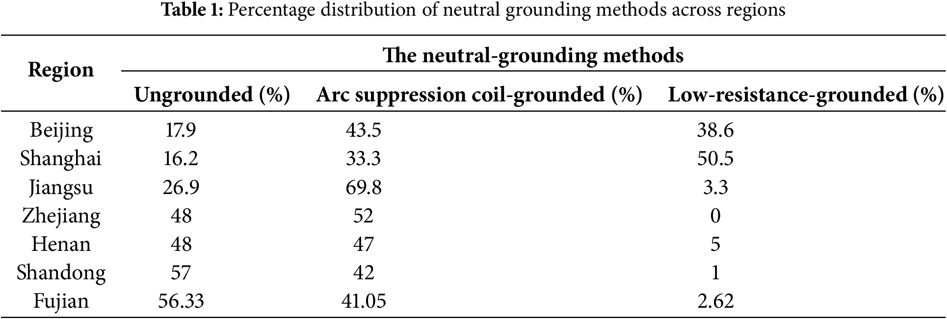
China’s medium-voltage distribution network is mainly used in the neutral point not grounded or by the arc-cancelling coil grounding small current grounding system, while some coastal economically developed areas of the test point is a large-current grounding system through the small resistance grounding. Such as Beijing, Shanghai and other economically developed areas, due to the cable usage rate increases year by year, the small resistance grounding method is gradually popularised, becoming the main neutral grounding method in such areas. Taking seven typical areas as a representative, specific data as shown in Table 1, the proportion of neutral point ungrounded, grounding through the arc-absorbing coil, small resistance grounding three grounding methods are: 39%, 47% and 14%, respectively.

Distribution line fault triggers can be divided into two categories: natural factors and human factors. Among them, natural factors mainly include lightning, bird damage, conductor ice, insulator dirt flash, hill fire and wind bias and other meteorological or environmental reasons; human factors cover the third-party damage, equipment aging failure, foreign body lap short circuit, engineering design defects, relay protection device triggered by error and operation and maintenance errors, etc. For example, lightning faults, foreign object lap faults and bird damage are defined as low-resistance grounding, while flashover along the surface of dirty insulators and tree line faults are defined as high-resistance faults. According to the data of 543 single-phase grounding faults occurred in a provincial power grid in three years, the cause of the fault is analysed in order to determine the type of grounding resistance, and the statistics of single-phase grounding fault resistance of low-resistance and high-resistance accounted for 76.61% and 23.36%, respectively.

The layout of the line is mostly in the form of triangular arrangement or horizontal parallel arrangement, resulting in an imbalance in the probability of faults occurring in different phases. Among them, phase B is usually located between phase A and phase C, so its relative probability of external interference is lower, which makes its probability of single-phase grounding fault is significantly lower than that of phase A and C. A power grid statistics show that the proportion of ground faults in phases A and C is 39.2% and 38.5%, respectively, and phase B is 22.3%.

These distribution characteristics provide critical parametric foundations for constructing class-imbalanced fault sample sets.

3  Single-Phase Grounding Fault Identification Based on CNN with CBAM Attention Mechanism

3.1 CBAM Attention Mechanism

The Convolutional Block Attention Mechanism sequentially integrates Channel Attention (CA) and Spatial Attention (SA) to weight features across both channel and spatial dimensions, thereby comprehensively mining feature importance and forming global attention regions. CBAM utilizes global pooling and convolutional operations to capture attention distributions in channel and spatial dimensions, respectively. Its structure is highly compatible with the feature extraction mechanisms of CNN, enabling seamless integration into deep networks such as ResNet. If Fig. 1 shows the input feature F∈RC×H×W processed by 1-dimensional channel attention Mc∈RC×1×1 and 2-dimensional spatial attention Ms∈R1×H×W as output, the overall attention process can be summarized as:

{F′=Mc(F)⊗FF′′=Ms(F′)⊗F′(1)

where ⊗ denotes element-by-element multiplication. During the multiplication process, the attention values are propagated accordingly.

Figure 1: CBAM attention mechanism diagram

(1) Channel attention

As shown in Fig. 2, the channel attention module simultaneously applies average pooling (AvgPool) and max pooling (MaxPool) to the input feature map, generating two channel descriptor vectors Favgc and Fmaxc, which represent the average and max pooled features, respectively. Subsequently, these descriptors are passed through a shared multi-layer perceptron (MLP) to produce the channel attention map Mc∈Rc×1×1. The MLP includes a hidden layer, whose activation size is determined by the reduction ratio r. Finally, the output feature vectors are combined by summation and activation functions. The channel attention is calculated as:

Mc(F)=σ(MLP(AvgPool(F))+MLP(MaxPool(F)))=σ(W1(W0(Favgc))+W1(W0(Fmaxc)))(2)

where σ denotes the Sigmoid function, W0∈RC/r×C, W1∈RC×C/r. The weights W0 and W1 of the MLP are shared for the two inputs and the ReLU activation function is used after W0.

Figure 2: Channel attention processing map

(2) Spatial attention

The spatial attention mechanism generates attention maps by leveraging spatial relationships of features, focusing on “where” information, which complements the “what” information captured by channel attention, thereby enhancing model generalization. As shown in Fig. 3, average pooling and max pooling are first applied along the channel dimension to generate two 2D feature maps, FavgS∈R1×H×W and FmaxS∈R1×H×W. These maps are concatenated and passed through a convolution layer to produce the spatial attention map Ms(F)∈RH×W, which emphasizes or suppresses specific regions. The spatial attention is computed as:

Ms(F)=σ(f7×7([AvgPool(F);MaxPool(F)]))=σ(f7×7([Favgs,Fmaxs]))(3)

where σ denotes a Sigmoid function and f7×7 denotes a convolution operation with a filter size of 7×7.

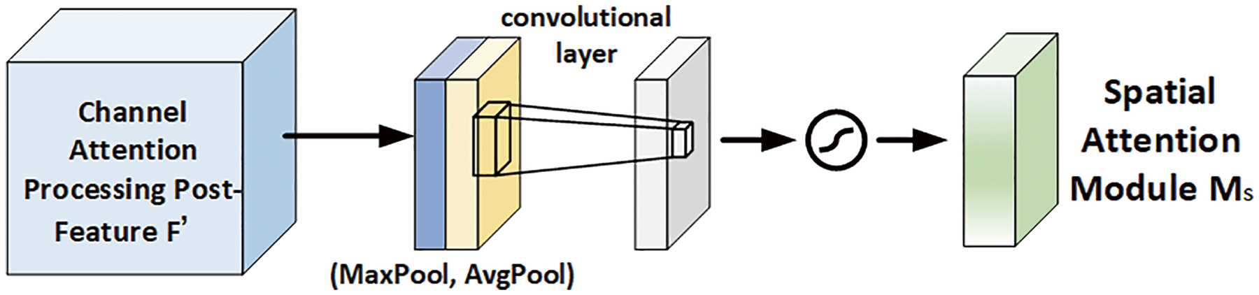
Figure 3: Spatial attention processing map

CBAM enhances feature extraction through global attention mechanisms across channel and spatial dimensions but cannot directly locate critical time segments. Given that zero-sequence current features exhibit significant non-smoothness and attenuation characteristics during fault initiation and termination phases, this study introduces a region-specific attention mechanism at these time segments. By amplifying key region features through trainable weights, the controllability of network is improved while incorporating prior knowledge.

Region-specific attention is achieved by constructing a binary mask Mseg specializing in the reinforcement of a specified row-column region, whose weights are adjusted by a trainable scalar γ. Let F′′∈RC×H×W denote the input feature map and Mseg∈{0,1}1×H×W denote the binary mask. The output is:

F′′′=F′′⊗(1+yMseg)(4)

where y is a learnable parameter that controls how much amplification is applied to the region.

3.2 CNN Model with CBAM Attention Mechanism

Convolutional Neural Networks is an effective deep learning method that consists of a multi-stage hierarchy of individual layers. From the input to the final classification layer, the input data passes through a series of trainable stages. Each stage applies linear or nonlinear operations to the input data to generate a feature map at the output. The multi-stage feed-forward process can be described as the following equation:

g(X)=gN(gN−1(…g2(g1(X;θ(1));θ(2))…;θ(N))(5)

where X represents the input data; θ(N) is the sequence of training parameters for each stage; gN is the activation function for each stage.

The CNN model in this study is constructed based on ResNet-18, whose backbone consists of convolutional layers, batch normalization (BN) layers, activation layers, and max pooling layers. To address noise interference and class imbalance issues, the network integrates a weighted random sampling module and a denoising module. CBAM modules are embedded after each residual block in ResNet-18 to adaptively enhance features from important channels and spatial regions. A SegmentAttention module is introduced after the final feature map to further amplify the weights of specific row-column regions, achieving deep integration of multiple attention mechanisms with ResNet-18. The overall network structure is shown in Fig. 4.

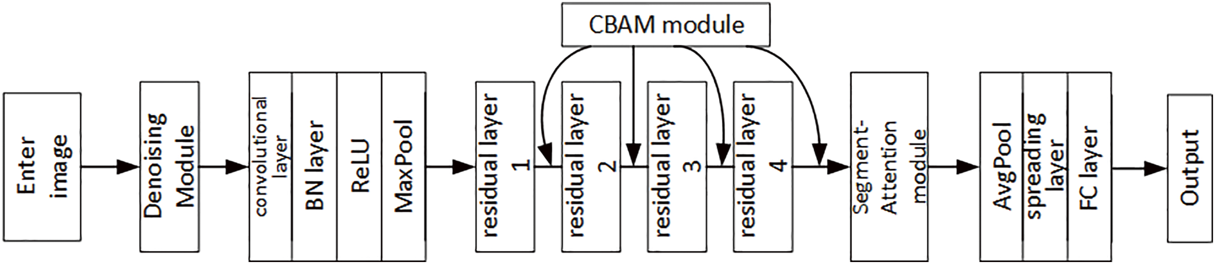
Figure 4: Diagram of the overall network structure of the CNN model

(1) Convolutional layer

The convolutional layer consists of a series of learnable kernels, the input is convolved with these learnable kernels to construct new feature maps which act as input to the next layer. Convolutional layer is used to extract feature maps from the input, the process of convolutional layer can be represented as:

Ymr,n=𝒮(∑pXpr−1×Kmr+Bmr)(6)

where Xpr−1 and Ymr,n denote the pth input feature map of stage e−1 and the mth output feature of stage r, respectively. Kmr is the convolution kernel between the pth input and mth output feature maps, n is the number of kernels or filters, and Bmr denotes the deviation of stage r.

(2) BN layer

The BN layer accelerates the network training process and reduces the internal covariate bias by standardizing the inputs of each layer so that the mean is 0 and the variance is 1, which makes the deep network easier to train, and at the same time, it has the regularization effect to a certain extent, which reduces the risk of overfitting and improves the stability of the model. Assuming that the input feature is X={x1,x2,…,xm}, its mean μ and variance σ2 are calculated and normalized to get x^i. The expressive ability of the model is restored by the learnable scaling parameter γ and offset parameter β, which are calculated as follows:

{μ=1m∑i=1mxiσ2=1m∑i=1m(xi−μ)2x^i=xi−μσ2+εyi=γx^i+β(7)

where ε is a very small constant preventing the denominator from being zero. γ and β control the variance and mean of the standardized data, respectively.

(3) ReLU

A nonlinear activation function (ReLU) is applied to the output of the convolutional layer to generate a feature map of the stage.

𝒴ijk=max(0,xijk)(8)

where xijk and 𝒴ijk are the i,j components of the kth input and output feature maps, respectively.

(4) Pooling layer

Pooling layers are critical components of convolutional neural networks, achieving dimensionality reduction and feature extraction on feature maps while preserving key information through spatial downsampling. By applying specific operators (e.g., max pooling or average pooling), they fuse adjacent features into a single value, thereby introducing spatial invariance and enabling the network to learn location-independent features. Maximum pooling can be expressed as follows:

𝒴y¯k¯=max(xif¯′k¯′:i≤l′<i+p,j≤j′<j+q)(9)

where p is the length and q is the width of the pooling window. In maximum pooling, the maximum value in the pooling window is selected to generate the output.

(5) Residual layer

Traditional deep networks directly learn the input-to-output mapping function H(x). However, as network depth increases, directly learning H(x) becomes challenging, resulting in degradation issues. ResNet introduces the concept of residual learning, addressing this problem by learning the residual function F(x)=H(x)−x (i.e., H(x)=F(x)+x) between inputs and outputs. Residual networks effectively mitigate the gradient vanishing/explosion problems that occur in deep convolutional networks (e.g., visual graphics network clusters) when the network layers are excessively deep. Fig. 5 illustrates a detailed 4-layer residual block in the ResNet-18 network.

Figure 5: ResNet18 network 4-layer residual block map

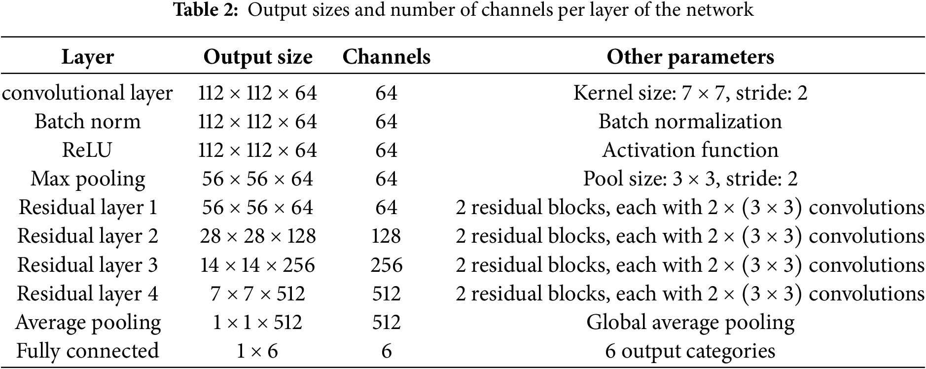
In the CNN architecture, convolutional layers and pooling layers are used to extract features from input data, while the fully connected layer (FC layer) maps the feature vectors to the output of category numbers. In this study, the FC layer is employed in the final stage of the network, consisting of a Dropout layer and a Linear layer for outputting classification results. The Dropout layer enhances the model’s regularization capability, effectively preventing overfitting. Table 2 presents the output dimensions and channel numbers for each layer of the network.

(6) FC layer and Dropout layer

In the CNN architecture, convolutional layers and pooling layers are used to extract features from input data, while the fully connected layer (FC layer) maps the feature vectors to the output of category numbers. In this study, the FC layer is employed in the final stage of the network, consisting of a Dropout layer and a Linear layer for outputting classification results. The Dropout layer enhances the model’s regularization capability, effectively preventing overfitting. Table 2 presents the output dimensions and channel numbers for each layer of the network.

To address noise interference in practical data, a denoising module is added before the ResNet network in this study. The module consists of an encoder and a decoder, as shown in Fig. 6. The encoder stacks two convolutional layers with nonlinear activation functions to extract multi-scale high-level features from the input image. The decoder employs a similar structure to restore the features to their original dimensions, thereby generating a denoised image. Each convolutional layer uses padding = 1 to ensure the spatial resolution of the feature maps remains unchanged.

Figure 6: Structure of denoising module

The input image be X, containing a clean signal S and noise N, the network goal is to learn a mapping function G(X) such that the output X^=G(X) is as close as possible to S. The convolutional layer extracts the core features of the image and filters out high-frequency noise; ReLU enhances the network’s ability to handle complex noise patterns. The mean square error (MSE) is used to minimize the error between the output and the clean image:

minGE[‖X^−S‖2](10)

To address the class imbalance problem in the dataset, where certain categories have significantly fewer samples than others, this study adopts a weighted random sampling method. First, the sample count nc for each category c is calculated, and a higher sampling probability pc∝1/nc is assigned to categories with fewer samples. During each training batch extraction, weighted sampling is performed based on pc∝1/nc, increasing the probability of selecting minority classes. By balancing the frequency of each category during the sampling phase without directly modifying the data, this method effectively mitigates the model’s bias toward majority classes while enhancing recognition capability for minority classes.

3.3 Grad-CAM Visualization and Analysis of CNN Models

To validate the effectiveness of the attention mechanism in improving the network’s recognition accuracy, this study employs Gradient-weighted Class Activation Mapping (Grad-CAM) to visualize the regions of interest in the input image for the CNN model, revealing its classification decision process. Grad-CAM quantifies the contribution of each feature map channel to the target category by calculating gradient information relative to the convolutional feature maps, thereby highlighting the most influential regions in the image for the model’s decision and providing an intuitive explanation for the prediction results. In implementation, the input image X is forward-propagated through the convolutional neural network to obtain the output feature maps of the target convolutional layer A; the score of the target category yc and its gradient ∂yc∂Aijk relative to the feature maps are calculated, followed by global average pooling of the gradient to derive the weights αkc.

αkε=1Z∑i∑j∂yϵ∂Aljk(11)

Following this, each feature map Ak is multiplied with the corresponding weight αkc to obtain a weighted feature map, and all the weighted feature maps are summed up and the ReLU activation function is applied to obtain the final Grad-CAM thermogram.

Lc=ReLU(∑kαkcAk)(12)

4  CBAM-CNN Based Single-Phase Ground Fault Identification Process

By analyzing the distribution network fault class imbalance problem, determine the system neutral grounding method, grounding resistance type and the percentage of faulted phases when the single-phase grounding fault occurs, collect the class imbalance data, train the CBAM-CNN fault identification model using SIMULINK fault simulation model, and verify the model’s accuracy and noise adaptability by using the simulation data and the recorded waveform data. Data volume for each type of single-phase ground-faults is shown in Table 3. The CBAM-CNN-based single-phase ground fault recognition process under class unbalance sampling is shown in Fig. 7, and the specific step flow is as follows.

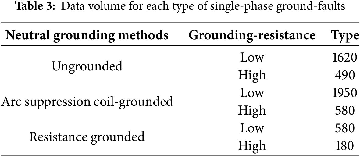
Figure 7: Flowchart of CBAM-CNN-based single-phase ground fault identification

Step1: By analyzing three neutral grounding methods, single-phase fault causes and phases in real-world grids to establish the proportional distribution of fault types. Then use a SIMULINK distribution network model and a MATLAB M-file for cyclic simulations to collect zero-sequence current data for various network structures, grounding methods, fault locations, phases, and resistor types.

Step2: By implementing code for the six grounding scenarios, we converted the corresponding zero-sequence current data into waveform images and saved them in separate folders. A CBAM-CNN fault recognition model is built, comprising denoising, attention, enhanced ResNet18, main program, and Grad-CAM visualization modules, then split the data 70:20:10 for training, validation, and testing, and conducted iterative training.

Step3: The test set is used to validate the model’s accuracy, and Grad-CAM is employed to confirm the correctness of the attention mechanism. Next, ablation studies verify the superiority of the proposed network architecture. Finally, field-recorded waveform images and test-set waveforms with added noise at varying signal-to-noise ratios are used to assess the adaptability and effectiveness of model in practical engineering applications.

5  Example Simulation and Experimental Analysis

5.1 Single-Phase Ground Fault Class Unbalanced Fault Sample Generation

In this section, the fault occurrence model of radial distribution network, ring distribution network and N supply and 1 standby distribution network is constructed in SIMULINK, as shown in Figs. 8–10. The main transformer is 110/10 kV, and the neutral grounding method of the main transformer can be set as ungrounded, grounded via arcing coil, and grounded via resistance. The parameters of the lines are shown in Table 4.

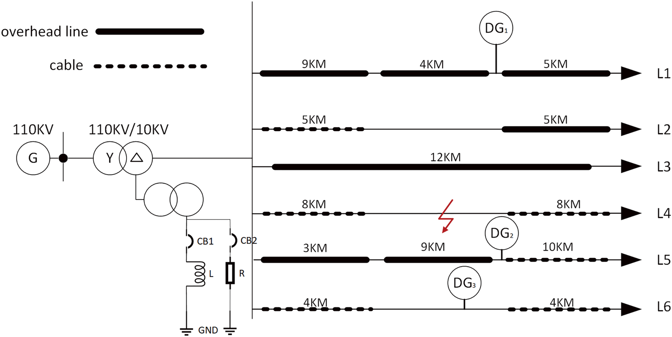
Figure 8: Structure of the 10 kV radial distribution network

Figure 9: Structure of a 10 kV ring-type distribution network

Figure 10: Structure of 10 kV N-supply and 1-standby type distribution network

As the probability of occurrence of different single-phase grounding fault types is considered, single-phase grounding faults are carried out in the three models respectively after changing the loop conditions of the MATLAB loop program, and in order to ensure that the simulation occurs after the stabilization of the distributed power supply, the faults are set to be in 0.8 s, and the zero-sequence current data are collected from 0.74 to 0.94 s with a sampling frequency of 10 kHz to simulate the different distribution network structures. The sampling frequency is 10 kHz to simulate different distribution network structures, neutral grounding methods, fault occurrence locations, fault occurrence phases and fault grounding resistance types. The network structure of the distribution network includes three types: radial, ring, and N-supply and 1-standby; the neutral grounding methods include three types of grounding methods: neutral ungrounded, grounded by arc-absorbing coil, and grounded by resistor; the fault locations include four cases: whether the fault occurs in the same feeder as DG and whether the fault location is between DG and the main power supply; the fault phases include three types of grounding: A-phase, B-phase, and C-phase; and the type of fault grounding resistor is classified as Low resistance grounding (1–500 Ω) and high resistance grounding (500–1000 Ω). According to the percentage of each type of situation identified in Section 1, i.e., 39%, 47%, and 14% of grounding methods, 77% and 23% of grounding resistance types, and 40%, 20%, and 40% of fault occurring phases, a total of 5400 sets of data were generated.

5.2 Comparison of Accuracy at Different Sampling Rates

In this paper, four common different sampling frequencies are used for comparison, and the results show that the accuracy of 10 kHz sampling frequency reaches 100%. Among the other three sampling frequencies, 4 kHz has limited bandwidth (Nyquist = 2 kHz), which is unable to capture high-frequency transient features; 6.4 kHz has an upper Nyquist frequency limit of only 3.2 kHz, which is difficult to capture the high-frequency transient features in the range of 3.2–5 kHz in single-phase earth faults. The Nyquist frequency limit of 6.4 kHz is only 3.2 kHz, which is difficult to completely capture the high-frequency transient features (e.g., steep drop of arc current, capacitive discharge oscillation) in the range of 3.2–5 kHz in single-phase grounding faults, resulting in the loss of key fault information; although the 20 kHz sampling rate can cover higher frequency band (Nyquist = 10 kHz), but it will multiplies the data volume and computation burden (the data volume of the same length of time is twice as much as that of 10 kHz), which puts forward more stringent requirements on the storage, transmission and real-time processing capabilities of edge computing devices, and reduces the deployment economy. The 10 kHz sampling is also more cost-effective to deploy in a single-phase system. Comparative results is shown in Table 5.

10 kHz sampling provides an optimal balance between accuracy and engineering feasibility in single-phase ground fault identification. It can effectively retain the transient features in the waveform that are crucial for classification (e.g., steep waveheads and arc oscillations at the beginning of the fault), and avoid the burden of data storage and computation caused by the high sampling rate, which is an efficient and sufficiently accurate choice for the current AI model to process the ground fault waveform data of the distribution network.

5.3 Single-Phase Ground Fault Identification Model Training and Result Analysis

The collected data is converted into waveform pictures with time as the horizontal axis and zero sequence current value as the vertical axis, which is used to train the fault identification model, a total of 15 rounds of training are performed, each round takes the data from the dataset, the prediction is obtained from the forward propagation and its loss is calculated, the backward propagation updates the model parameters, and finally, the average loss and the accuracy of the round are counted, and the optimizer is used is Adam with a learning rate of 0.001, Batch size is 32, the training process fold is shown in Fig. 11. In this paper, recall, precision, F1 score, and confusion matrix are used as model evaluation metrics to assess the effectiveness of the fault identification model on the test set. Table 6 shows the scores of various evaluation metrics for the models trained in this paper, and Fig. 12 shows the confusion matrix for fault recognition model test set.

Figure 11: Line graph of the training process

Figure 12: Fault recognition model recognition confusion matrix

In order to observe the influence of each location in the image on model discrimination, as well as to verify the effectiveness of the attention mechanism in a specific region, this paper calculates the weight akc of each channel through the Grad-CAM visualization method, and superimposes each feature map Ak by multiplying it with the corresponding weight akc to generate the Grad-CAM heat map. As shown in Fig. 13, the input waveform images of the two sets of data and their Grad-CAM heat maps are shown. The color intensity of the heat map corresponds to the discriminative influence, and the closer the pixel color tends to be to the warmer color, the higher the influence of this location on the discriminative decision, which can be observed intuitively that the warmest color locations in Fig. 13a, b are located in the time of the fault just occurring and the time of the attenuation, which is in line with the description of the previous section.

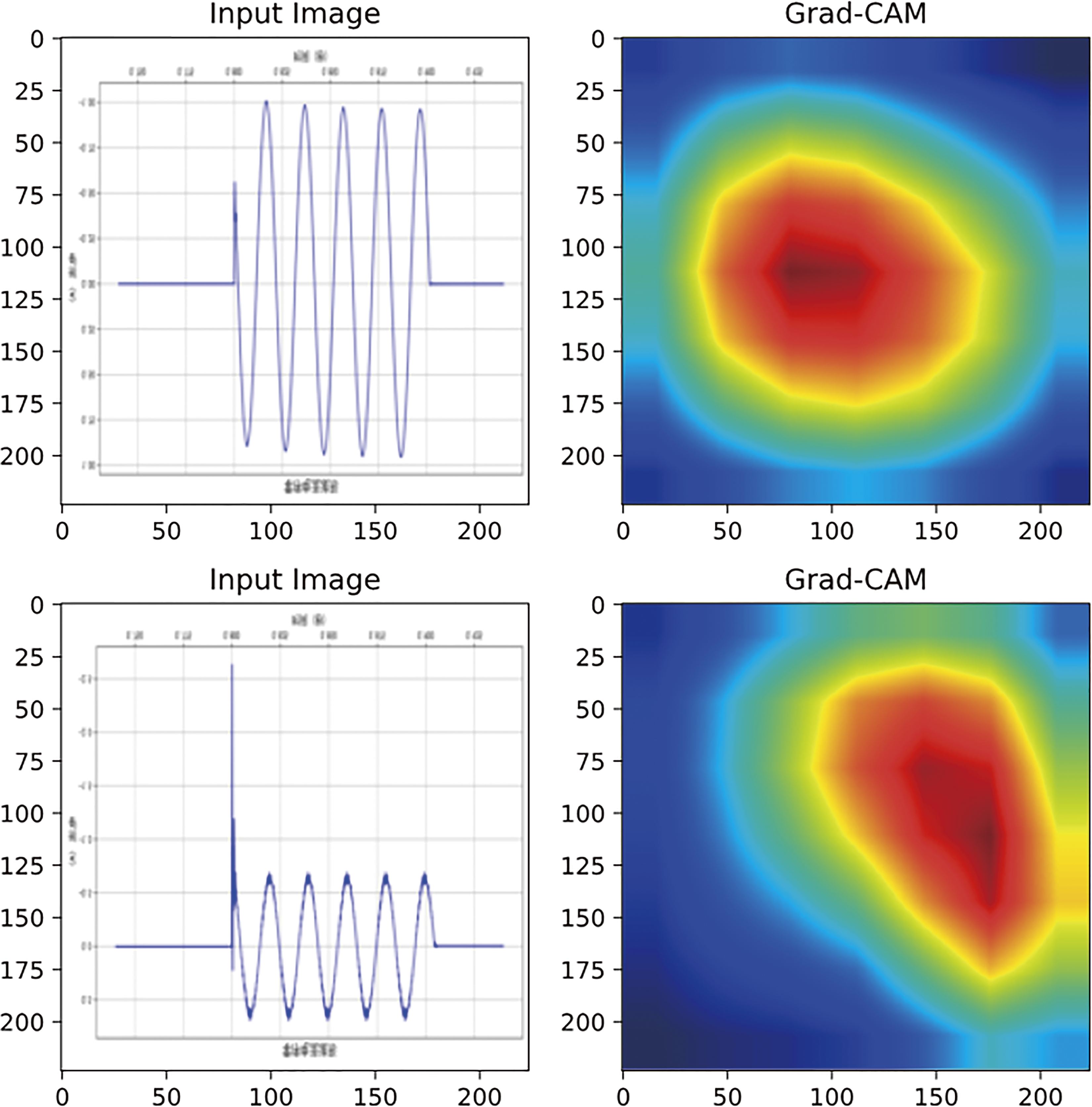
Figure 13: Input waveform image and its Grad-CAM heat map

5.4 Comparative Analysis of Algorithms

In order to verify the effectiveness of the proposed model in this paper, the following comparative analysis is carried out in three aspects, namely, weighted random sampling module, attention module and CNN network model, respectively, as shown in Table 6, where cases 1–3 aim to verify the importance of data imbalance processing and correctly adding attention to the image feature locations, and cases 4–5 aim to verify the selected CNN network in this paper’s superiority. Comparative analysis of algorithms are are shown in Table 7.

As Fig. 14 shows the recognition accuracies of various cases on the test set, the accuracies of cases 1–3 are all slightly lower than this paper’s method, so the other modules added to the ResNet18 base network in this paper all play a positive role. However, when the ResNet18 network is replaced by the AlexNet network, the recognition accuracy drops to 61.18%, which may be due to the lack of feature lifting ability of AlexNet, and as the network becomes more complex, there is a problem of feature confusion, gradient convergence is difficult and easy to collapse, and it requires more epochs and a larger Batch size in order to train the desired results. The recognition accuracy of case 5 is 99.44%, in the network without residual structure, the gradient keeps decaying or exploding in the backpropagation, which causes the training to become difficult, while the residual connection allows the network to remain trainable when the number of layers increases, which results in higher expressiveness and better accuracy for deeper layers of the network.

Figure 14: Recognition accuracy for each comparison case

5.5 Noise Immunity Analysis

In order to simulate the noise signals that often occur in real engineering, this paper adds noise with signal-to-noise ratios of 10, 20, 30, and 40 dB to each sample of the test set for the noise immunity of this paper’s method, respectively. The recognition accuracy under different noise levels is shown in Table 8, and the recognition accuracy can reach 100% when the signal-to-noise ratio is 40 dB, and with the increase of the noise percentage, the recognition accuracy can still be maintained at a high level, indicating that the model has good adaptability to data noise.

5.6 Test and Recording Data Validation

In order to further verify the applicability of the proposed CBAM-CNN identification model in practical engineering applications, this paper records 6 sets of recorded waveform data (3 sets for each of the 2 grounding modes) and collects 28 sets of fault data for 10 kV lines in different prefectures of a provincial grid after conducting experiments of single-phase low-resistance ground faults with neutral point not grounded and grounded via an arcing coil in a true-type test field of the distribution network. Among them, Fig. 15 shows a set of experimental zero-sequence current waveforms when the system neutral is not grounded and when it is grounded via the arcing coil, respectively, while Fig. 16 shows a set of three-phase current waveforms and their corresponding zero-sequence current waveforms for 10 kV line data.

Figure 15: Experimental recorded waveforms for single-phase ground faults

Figure 16: Structure of denoising module

The confusion matrix of the recognition results is shown in Fig. 17. The algorithm in this paper can completely and correctly identify this set of experimental data with the measured data, because the CBAM-CNN model can automatically extract multi-level features from the original waveforms, capture local patterns and global structure, and mine hidden features to reduce the under-reporting of fault information. Fig. 17 The performance results of the confusion matrix identified by the test and record data are shown in Table 9.

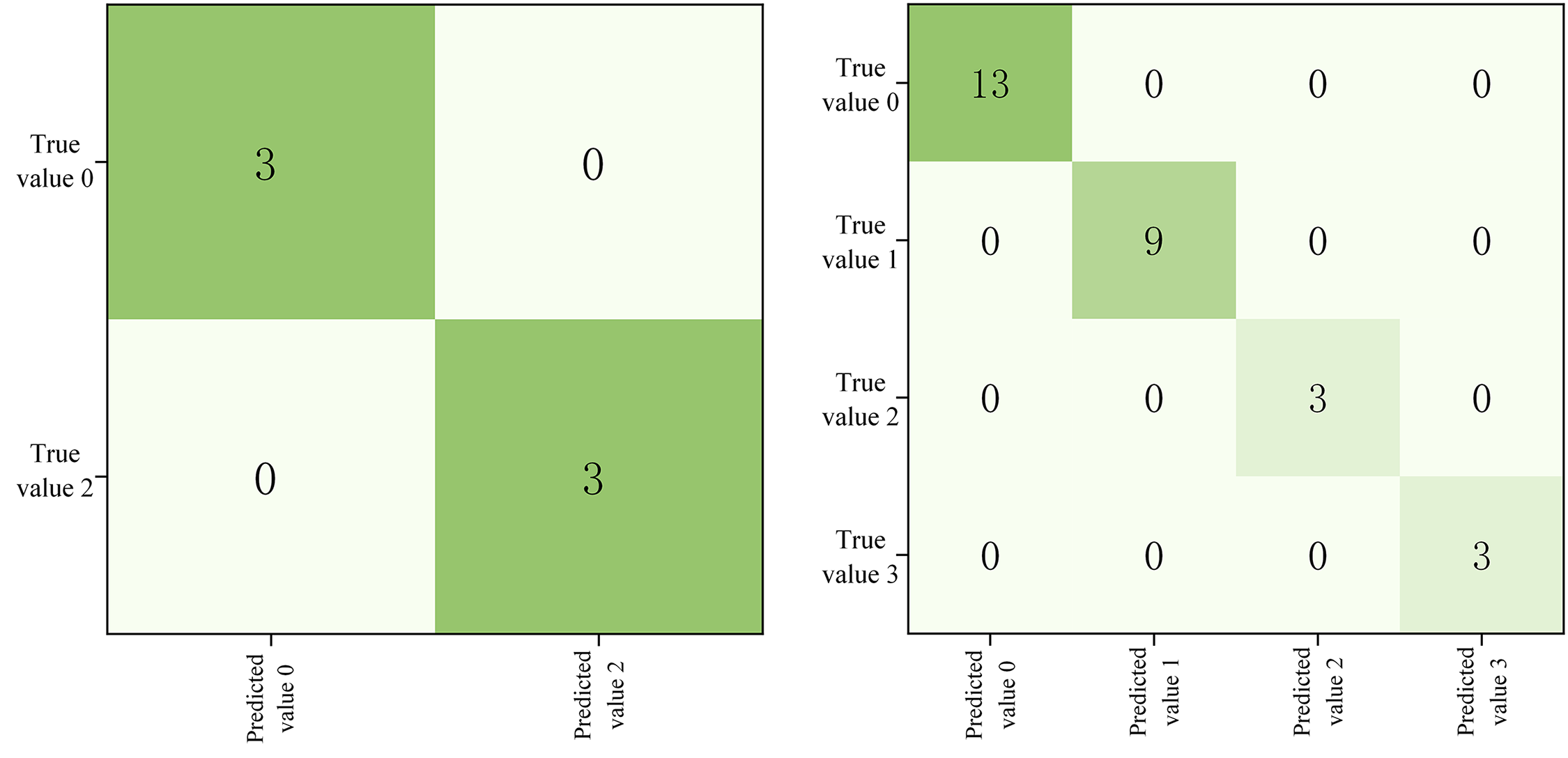
Figure 17: Confusion matrix for test and recording data identification

5.7 Ablation Experiment Result Analysis

To verify the contribution of the CBAM module to model performance, this study conducted an ablation experiment comparing the Baseline_ResNet18 model with the CBAM_ResNet18 model under identical training conditions. The results are shown in Table 10. The experiment evaluates the models from three dimensions: test accuracy, convergence efficiency, and training cost. Additionally, other mainstream models such as SE_ResNet18 and ResNet50 are compared to further validate the effectiveness, as illustrated in Fig. 18.

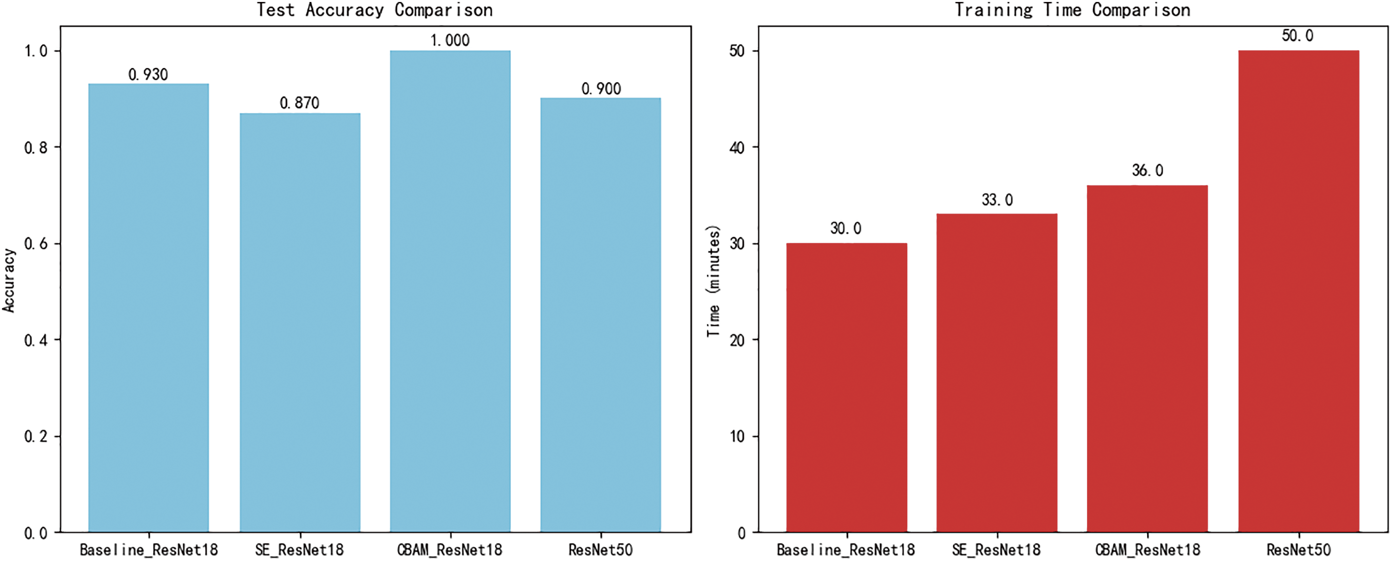
Figure 18: Comparison of test accuracy and training time across multiple models

In terms of test accuracy, CBAM_ResNet18 significantly outperforms other models with an absolute accuracy of 100%, compared to 93.0% for Baseline_ResNet18, 87.0% for SE_ResNet18, and 90.0% for ResNet50. This validates the effectiveness of the channel-spatial attention mechanism in enhancing the extraction of fault features. Regarding training time, CBAM_ResNet18 completes training in just 36.0 min. Although this is a 20% increase compared to the lightweight baseline, it saves 28% in training time compared to ResNet50, demonstrating a balanced advantage between accuracy and efficiency.

5.8 Comparative Analysis of Different Attention Mechanisms and Network Architectures

This experiment validates the superiority of the CBAM attention mechanism in power equipment fault diagnosis tasks through a comprehensive comparison of multi-dimensional model performance. A dual-dimensional evaluation framework is adopted: in the attention mechanism dimension, the integration effects of SE, CBAM, and no attention mechanism within the ResNet18 architecture are compared; in the network architecture dimension, the performance differences between ResNet18 and ResNet50 are evaluated. The comparative experiment benchmarks the CBAM attention mechanism against other classical attention mechanisms and network architectures, verifying its superiority and applicability. All models are validated under consistent experimental conditions, and the final results are presented in Table 11.

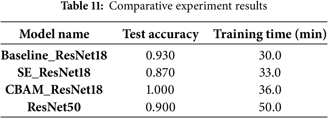
In the task of power equipment fault diagnosis, CBAM_ResNet18 demonstrates comprehensive performance superiority. It achieves a 100% test accuracy, significantly surpassing all baseline models and achieving a 7% absolute accuracy improvement over the baseline model, Baseline_ResNet18. At the same time, it maintains an efficient training time of 36.0 minutes—only a 20% increase compared to the lightweight baseline, yet achieving a 28% reduction in computational cost compared to the deeper ResNet50 network. Notably, SE_ResNet18 exhibits an unexpected performance degradation, with accuracy dropping to a suboptimal 0.870, revealing the inherent limitations of single-channel attention mechanisms in power waveform diagnosis. Meanwhile, ResNet50 suffers from overfitting tendencies and excessive computational burden, significantly weakening its cost-effectiveness for practical deployment. This comparative experiment fully verifies that CBAM’s dual attention mechanism, achieves a breakthrough in diagnostic accuracy and enhances model robustness, all within a controllable training time.

6  Conclusion

This paper addresses the class-imbalance problem of single-phase ground-fault samples in distribution networks with distributed generation by proposing a CBAM-CNN fault recognition method. Construct imbalanced sample sets of zero-sequence current waveform images according to real-world fault probability distributions and train a CBAM-CNN model applicable to various network topologies. The model’s high accuracy is validated using both simulation data and field-recorded waveforms.

Key conclusions are as follows. The CBAM-ResNet18 architecture maintains trainability in deep layers via residual connections and enhances feature representation by channel-wise attention. Grad-CAM visualizations reveal that the network focuses primarily on the fault inception and decay phases. Ablation studies and noise-augmentation experiments confirm the model’s superiority and strong noise robustness. And the proposed model achieves 100% fault identification accuracy on both recorded data and simulated data across three different distribution network structures, outperforming existing methods in precision.

Acknowledgement: We hope that this study will be of interest to your journal. Thank you in advance for your consideration.

Funding Statement: This work is supported by the Science and Technology Program of China Southern Power Grid (031800KC23120003).

Author Contributions: The authors confirm contribution to the paper as follows: study conception and design: Lei Han and Wanyu Ye; data collection: Chunfang Liu and Siyuan Liang; analysis and interpretation of results: Lei Han and Shihua Huang; draft manuscript preparation: Chun Chen, Luxin Zhan and Wanyu Ye. All authors reviewed the results and approved the final version of the manuscript.

Availability of Data and Materials: Due to the nature of this research, participants of this study did not agree for their data to be shared publicly, so supporting data is not available.

Ethics Approval: Not applicable.

Conflicts of Interest: The authors declare no conflicts of interest to report regarding the present study.

Nomenclature

References

1. Zhang X, Bie Z, Li G. Reliability assessment of distribution networks with distributed generations using monte carlo method. Energy Proc. 2011;12:278– 286. doi:10.1016/j.egypro.2011.10.038. [Google Scholar] [CrossRef]

2. Ekwue AO, Akintunde OA. The impact of distributed generation on distribution networks. Niger J Technol. 2015;34(2):325. doi:10.4314/njt.v34i2.17. [Google Scholar] [CrossRef]

3. Misshra M, Routray P, Rout P. A universal high impedance fault detection technique for distribution system using s-transform and pattern recognition. Technol Econ Smart Grids Sustain Energy. 2016;1(1):9–18. doi:10.1007/s40866-016-0011-4. [Google Scholar] [CrossRef]

4. Salim RH, Oliveira K, Filomena AD, Resener M, Bretas A. Hybrid fault diagnosis scheme implementation for power distribution systems automation. IEEE Trans Power Deliv. 2008;23(4):1846–56. doi:10.1109/tpwrd.2008.917919. [Google Scholar] [CrossRef]

5. Sedighi AR, Haghifam MR, Malik OP, Ghassemian H. High impedance fault detection based on wavelet transform and statistical pattern recognition. IEEE Trans Power Deliv. 2005;20(4):2414–21. doi:10.1109/tpwrd.2005.852367. [Google Scholar] [CrossRef]

6. Li Y, Zhang Y, Liu W, Chen Z, Li Y, Yang J. A Fault pattern and convolutional neural network based single-phase earth fault identification method for distribution network. In: 2019 IEEE Innovative Smart Grid Technologies Asia(ISGT Asia); 2019 May 21–24; Chengdu, China. p. 838–43. doi:10.1109/isgt-asia.2019.8881610. [Google Scholar] [CrossRef]

7. Biswas S, Nayak PK, Panigrahi BK, Pradhan G. An intelligent fault detection and classification technique based on variational mode decomposition-CNN for transmission lines installed with UPFC and wind farm. Elect Power Syst Res. 2023;223(3):109526. doi:10.1016/j.epsr.2023.109526. [Google Scholar] [CrossRef]

8. Wang X, Wei X, Yang D, Song G, Gao J, Wei Y, et al. Fault feeder detection method utilized steady state and transient components based on FFT backstepping in distribution networks. Int J Electr Power Energy Syst. 2020;114(5):105391. doi:10.1016/j.ijepes.2019.105391. [Google Scholar] [CrossRef]

9. Zeng P, Li H, He H, Li S. Dynamic energy management of a microgrid using approximate dynamic programming and deep recurrent neural network learning. IEEE Trans Smart Grid. 2019;10(4):4435–45. doi:10.1109/tsg.2018.2859821. [Google Scholar] [CrossRef]

10. Ibitoye OT, Oni-Bonoje MO, Dada JO. Machine learning based techniques for fault detection in power distribution grid: A review. In: 2022 3rd International Conference on Electrical Engineering and Informatics (ICon EEI); 2022 Oct 19-20; Pekanbaru, Indonesia. p. 104–7. [Google Scholar]

11. Jia YX, Liu Y, Wang BL, Lu DY, Lin YZ. Power network fault location with exact distributed parameter line model and sparse estimation. Elect Power Syst Res. 2022;212(6):108137. doi:10.1016/j.epsr.2022.108137. [Google Scholar] [CrossRef]

12. Meydani A, Shahinzadeh H, Ramezani A, Moazzami M, Askarian-Abyaneh H. Comprehensive review of artificial intelligence applications in smart grid operations. In: 2024 9th International Conference on Technology and Energy Management (ICTEM); 2024 Feb 14–15; Beh Shar, Mazandaran, Iran. p. 1–13. [Google Scholar]

13. Zhang J, Li Y, Zhang Z, Zeng Z, Duan Y, Cao Y. XGBoost classifier for fault identification in low voltage neutral point ungrounded system. In: 2019 IEEE Sustainable Power and Energy Conference (ISPEC); 2019 Nov 21–23; Beijing, China. p. 1767–71. [Google Scholar]

14. Zhu J, Mu L, Ma D, Zhang X. Faulty line identification method based on bayesian optimization for distribution network. IEEE Access. 2021;9:83175–84. doi:10.1109/access.2021.3087131. [Google Scholar] [CrossRef]

15. Zhang R, Li C, Jia D. A new multi-channels sequence recognition framework using deep convolutional neural network. Procedia Comput Sci. 2015;53:383–95. [Google Scholar]

16. Selvaraju RR, Cogswell M, Das A, Vedantam R, Parikh D, Batra D. Grad-CAM: visual explanations from deep networks via gradient-based localization. In: 2017 IEEE International Conference on Computer Vision (ICCV); 2017 Oct 22–29; Venice, Italy. p. 618–26. doi:10.1109/ICCV.2017.74. [Google Scholar] [CrossRef]

17. Tan PN, Steinbach M, Karpatne A. Classification: basic concepts and techniques. In: Introduction to data mining. 2nd ed. London, UK: Person; 2019. p. 113–92. [Google Scholar]