Multi-Scenario Probabilistic Load Flow Calculation Considering Wind Speed Correlation

1  Introduction

As the energy issue becomes increasingly severe, clean energy has become a hot topic in current research. As the penetration of new energy in distribution networks continues to rise, safety issues such as voltage violations and power flow overloads are becoming increasingly severe. In high-proportion new energy-penetrated distribution networks, data-driven methods can be used for short-term, high-precision node voltage sensing and prediction, even without a power flow model [1]. State estimation technology ensures the safe operation of the grid by sensing the current operating state of AC and DC distribution networks and predicting voltage trend changes. Xu et al. conducted a quantitative analysis and characterization of measurement uncertainty in the system using interval numbers and established a more comprehensive interval state estimation (SE) model [2]. The three-phase interval SE model, described in interval form for distributed energy output and measurements, can provide the entire range of system states under the influence of multiple uncertain factors [3].

Correlation factors can affect load demand, power output characteristics, and system operation mode, which significantly impact the operation of the power system. Therefore, considering wind speed correlation is significant for probabilistic load flow (PLF) calculation and dispatch operation planning [4–6]. The main methods to solve the correlation of random variables are Polynomial Normal transformation, Rosenblatt transformation, Nataf transformation, and Copula Function. The Monte Carlo Simulation (MCS) method requires sacrificing computation time to achieve accuracy and is typically used to validate the accuracy of other methods [7,8]. The basic principle of the point estimation method is the same as that of MCS, but the sample size is smaller than that of MCS. Combining numerical statistical methods can improve efficiency. The disadvantage of the point estimation method is that when the system node size is considerable, the number of power flow calculations also increases, which may result in lower computational efficiency [9].

The cumulant method (CM) uses the cumulant of the stochastic model to transform the complex convolutional computation into a simple algebraic operation when the input variables are independent, making the computation speed much higher. It is widely used in the fields of power market [10], power system PLF analysis, and distributed generation optimal allocation [11–13]. High wind power penetration causes the state variables in PLF calculations to no longer follow a normal distribution, making the traditional Gram-Charlier and Cornish-Fisher series expansion methods unsuitable [14]. Reference [15] combines the C-type Gram-Charlier (CGC) series based on the multipoint linearization method to avoid the issue of negative values in the probability density function (PDF) of system state variables when using the A-type Gram-Charlier (AGC) series in high wind power penetration. The maximum entropy principle can improve computational accuracy by iteratively correcting the PDF of the traditional CGC method [16]. By discretizing the injection power of wind farms in segments, the PLF calculation can be converted into multiple PLF calculation problems that follow normal distributions, which can avoid the problem of violating probability axioms during series expansion [17,18].

When the penetration rate of wind power is high, the above literatures study how to improve the computational accuracy of CM based on the assumption that wind speeds are mutually independent. Neglecting the correlation between wind speeds can significantly increase the error in PLF calculations. To address this gap, this paper considers wind speed correlation in the CM power flow calculation. The main contributions of this study are shown as follows:

(1) Adopting a random sampling method to obtain the output probability of discrete scenarios overcomes the limitation of traditional discretization methods, which can only calculate the output probability of discrete scenarios in uncorrelated cases by defining independent events.

(2) The Nataf transformation is used to handle the correlation between wind speeds, generating correlated samples. Combined with random sampling, this method obtains the output probability of discrete scenarios, enabling the traditional cumulant-based power flow calculation method for discretized wind farm power to address correlation issues.

(3) Using the law of total probability to derive the probability density curve in correlated scenarios avoids the issue of inaccurate fitting of the probability density curve associated with series expansion methods.

2  Discretization Model of Wind Farm

2.1 Active Power of Wind Farm

The PDF of wind speed v typically satisfied the two-parameter Weibull distribution, as shown in Eq. (1). The active output of the wind turbine is determined by the wind turbine’s cut-in wind speed vci, rated wind speed vr, and cut-out wind speed vco, whose relationship is shown in Eq. (2).

f(v)={βηβexp⁡((−vη)β)v>00v≤0(1)

P(v)={0v<vci,v≥vcoPwv−vcivr−vcivci≤v<vrPwvr≤v<vco(2)

where η represents the shape parameter, β is the scale parameter, and Pw represents the rated power of the wind turbine.

2.2 Construction of Multi-Scenario Wind Power Output Power

Section 2.1 shows that the wind turbine’s active output includes zero output, rated output, and linear region, as shown in Fig. 1. According to the method in Reference [17], the linear range is divided into l segments based on the set power step Pt, where the power output value for each segment is the expected power value Pmi (i = 1, 2, …, l) of that segment. The discrete point Pm0 = 0 corresponds to the state when the output power is 0, and the discrete point Pm(l+1) = 0 corresponds to the state when the output is at rated power Pw. Therefore, according to Eq. (3), l + 2 discrete points can be obtained [17].

Pmi={0i=0(i+12)Pti=1,2,⋯,lPwi=l+1(3)

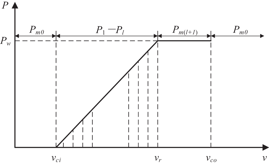
Figure 1: Schematic diagram of wind farm active power discretization

The wind farm operates under constant power factor conditions. Randomly combining the discretized wind power will yield discrete scenarios of wind power. The total number of scenarios W can be calculated by Eq. (4), while Eq. (5) provides the active power of each wind farm in the corresponding scenarios.

W=∏j=1N(mj+2)(4)

Sk={P1(Sk),⋯Pj(Sk),⋯PN(Sk)},k∈[1,W](5)

where N denotes the number of wind nodes, mj denotes the number of discrete segments the j-th wind farm, Pj (Sk) is the output of the j-th wind farm in the k-th scenario.

3  Correlation Processing of Input Variables

3.1 Correlation Model of Wind Speed

The Pearson correlation coefficient matrix of the random variable vector Vm×1=[v1,…,vm] is ρv as shown in Eq. (6). The matrix element ρvij can be obtained from Eq. (7).

ρv=[1ρ12⋯ρ1mρ211⋯ρ2m⋮⋮⋱⋮ρm1ρm2⋯1](6)

ρvij=ρ(vi,vj)=Cov(vi,vj)σiσj=Cov(vj,vi)σjσi=ρvji(7)

where σi and σj represent the standard deviation (SD) of the random variables vi and vj, respectively, and Cov (vi,vj) denotes the covariance of the random variables vi and vj.

Based on the wind speed samples generated by the inverse Nataf transformation, the active power output samples of the wind turbine can be obtained using Eq. (2). The basic steps of inverse Nataf transformation to generate wind speed samples satisfying a given Pearson correlation coefficient and PDF are as follows [19]:

(1) Generate samples Ys of independent standard normal distribution random variable vector Ym×1.

(2) Following the Pearson correlation coefficient matrix ρv of the wind speed Vm×1 and the equivalent correlation coefficient empirical calculation formula shown in Eq. (8), the Pearson correlation of the standard normal distribution random quantity vector Xm×1 with correlation is obtained. Cholesky decomposes the coefficient matrix ρx to obtain Gx, which can be calculated as

ρxij=D(ρvij)ρvij(8)

ρx=GxGxT(9)

(3) Sample Xs of a standard normally distributed random variable vector Xm×1 with a Pearson correlation coefficient matrix of ρx is obtained through Eq. (10).

Xs=GXYs(10)

(4) The sample Vs of the wind speed vector Vm×1, whose Pearson correlation coefficient matrix is ρv and PDF is f(v), can be generated by the principle of equal probability conversion, as shown in Eq. (11).

Vs=F−1(Φ(Xs))(11)

3.2 Output Probability of Discretized Scenarios

Let ξ1, ξ2,…, ξn… be independent and identically distributed random variable sequences, and have mathematical expectations and variances: Eξi=μ, Dξi=σ2(i=1, 2, …, n…), then for any given ε>0, the arithmetic mean of the random variable converges to its mathematical expectation value with probability, as shown in Eq. (12).

limn→∞P{|1n∑i=1nξi−μ|<ε}=1(12)

In scenario Sk, when each wind power node is independent, the probability pjk of wind farm Pj(Sk) can be obtained using Eq. (1), and the output probability pk of the k-th scene of the wind farm can be obtained by Eq. (13).

pk=∏j=1Npjk(13)

When the wind power nodes are correlated, n sets of correlated active power samples can be generated using the method in Section 3.1. All discrete scenes of the wind farm constitute the state space Ω, and each scene corresponds to a subspace Ωk of the state space. When the number of wind power samples corresponding to subspace Ωk in scenario Sk is known, the output probability pk of the corresponding scenario can be calculated using Eq. (14).

pk=nkn(14)

4  Probabilistic Power Flow Calculation

4.1 Semi Invariant Method

The Taylor series expansion of the node injection power equation and the branch power flow equation of the AC power flow model in polar coordinate form is done at the reference operating point, ignoring the high-order items of degree 2 or above, and the results are as follows:

{X=X0+ΔX=X0+S0ΔWZ=Z0+ΔZ=Z0+T0ΔW(15)

where W is the node injected power; X is the node state variable; Z is the branch power flow variable (including branch active and reactive power); J0 is the Jacobi matrix for the power flow calculation; S0 and T0 are the sensitivity matrices, with S0=J0−1, T0=G0J0−1, G0=(∂Z/∂X)|X=X0.

All other nodes are load PQ nodes except for a single conventional power supply node as a balancing node in the power distribution network. There are only normally distributed random variables P and Q in the network when line faults and outages of the superior power grid are not considered. All cumulants above the second order are zero for a random variable that follows a normal distribution. The linear combination of the random variables with a normal distribution still meets the normal distribution. To avoid a large number of calculations of convolution, according to the property of cumulant, we have

ΔW(k)=ΔWG(k)−ΔWL(k)(16)

{ΔX(k)=S0(k)ΔW(k)ΔZ(k)=T0(k)ΔW(k)(17)

where ΔW(k) is the kth-order cumulant of the injected power at the node; ΔW(k)G and ΔW(k)L are the kth-order cumulants of the variations of generator power and load power, respectively; ΔX(k) and ΔZ(k) are the kth-order cumulants of the variations of the state variables, respectively; and S0(k) and T(k)0 are the matrices consisting of the kth powers of the elements of the matrices S0 and T0, respectively.

4.2 State Variables of Wind Power Injection Scenario

In the absence of line faults and power grid outages, assuming that wind farm power and load power are independent and that the output power at the wind power nodes is constant in discrete scenarios, the conditional probability of the state variables in the probabilistic power flow calculation still follows a normal distribution. The only difference from power flow calculations that consider only load randomness is that the operating reference point shifts due to the injection of wind power. When performing cumulant-based power flow calculations with discretized wind farm power, the higher-order cumulants (above the second order) of state variables are all zero. Only the second-order cumulants of the state variables need to be calculated. The cumulative distribution function (CDF) of the conditional event A|Bk is shown in Eq. (18), where event A represents the state variable x being less than xA, and Bk indicates the wind power output in the kth state Sk. According to the total probability Eq. (19), the CDF of event A is Eq. (20), and the PDF is Eq. (21).

F(xA∣Bk)=∫−∞xA1σk2πexp⁡[−(t−μk)22σk2]dt(18)

Prob(A)=∑k=1WProb(A∣Bk)×pk(19)

F(xA)=∑k=1W{Prob(Bk)∫−∞xA1σk2πexp⁡[−(t−μk)22σk2]dt}(20)

f(xA)=∑k=1W{Prob(Bk)1σk2πexp⁡[−(xA−μk)22σk2]}(21)

where F(xA|Bk) is the probability that the state variable x is less than xA in the k-th state of wind power output (cumulative probability); μk and σk are the mean and SD of the state variable x obtained from the calculation of probability currents considering the stochastic change of loads in the k-th state of the system wind power output.

4.3 State Variables of Wind Power Injection Scenario

When there is correlation between wind speeds, obtaining the output probability of each scenario through analytical methods becomes complex. The only difference between different discrete scenarios under different wind speed correlations is that the output probability of each discrete scenario is different. The random sampling method was used to obtain the output probability of each scenario. The PLF calculation flowchart is shown in Fig. 2, and the steps of the PLF calculation process are described as follows:

(1) Discretize each wind farm power according to the discretization step size and randomly combine the discrete points of each wind farm power to construct all discrete scenarios.

(2) The active power output samples of the wind turbine are obtained using the method described in Section 3.1. The ratio of the number of active power samples contained in a single scenario to the total sampling times represents the output probability of that scenario.

(3) After discretization, if the wind power in a single scene is constant and the system only contains loads with normal distribution, W sets of PDF and CDF that follow normal distribution can be obtained.

(4) The final power flow calculation result can be obtained by weighting and superimposing the power flow calculation results that only consider the randomness of the load in each discrete scenario according to the output probability of the corresponding discrete scenario.

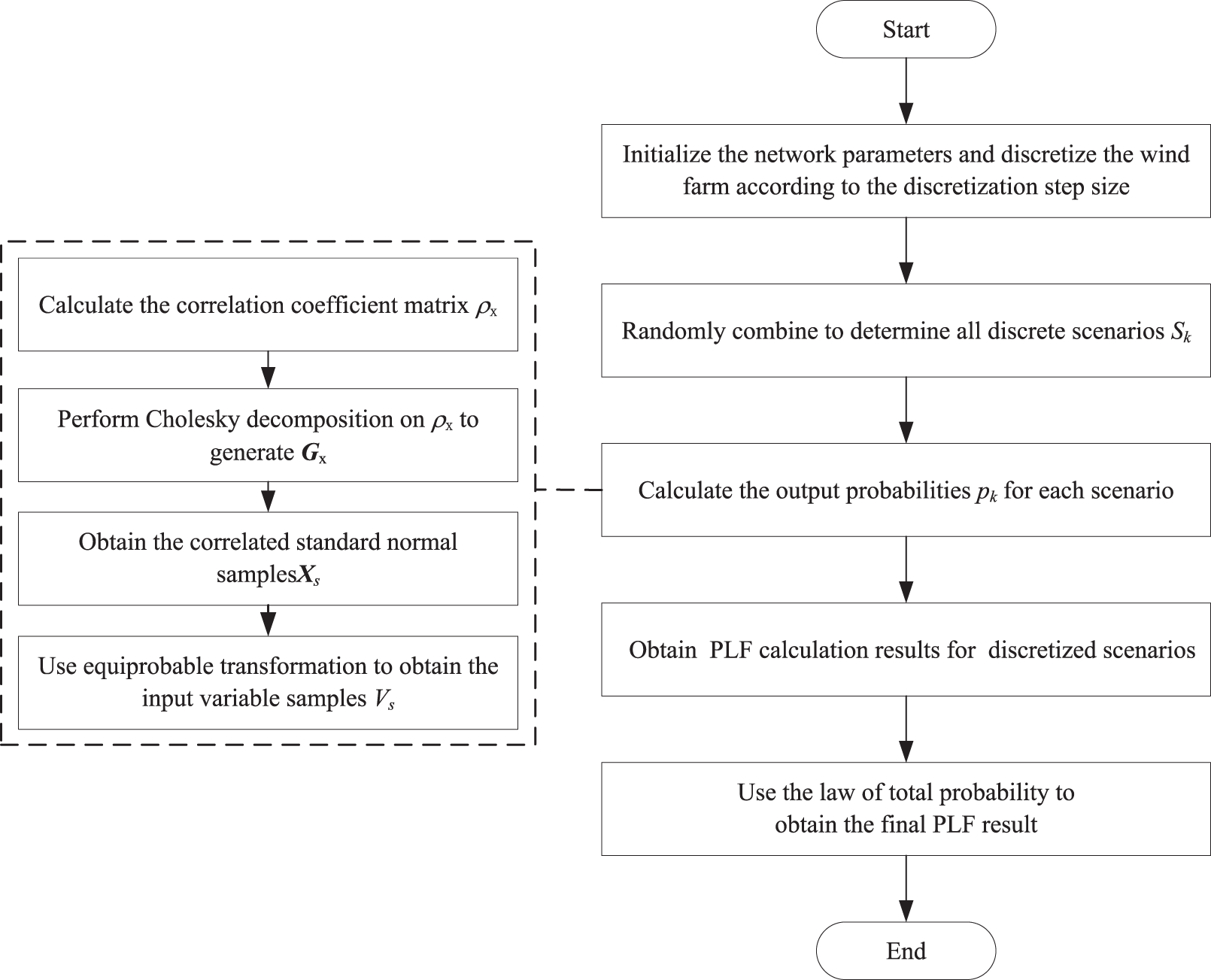
Figure 2: Power flow calculation flowchart

5  Example Analysis

5.1 Calculation Introduction

In Section 5.2, the accuracy of the random sampling method for calculating the output probability of discrete scenarios is validated. In Section 5.3, the precision of the proposed PLF calculation method is confirmed. In Section 5.4, the effectiveness of the process in handling correlation issues is demonstrated. The expected values of the node loads are taken as the original fixed system loads, with a standard deviation of 10% of the mean. The power factor of the wind farms is a constant value of 0.98, vci = 3 m/s, vr = 15 m/s, vco = 25 m/s, η = 10, β = 2. The discretization step size is 0.25 MW.

5.2 Calculating the Output Probability of Wind Power Scenarios

The probability of wind power outputs for each scenario can be obtained using the PDF of wind speeds for the wind farms when their outputs are independent. Using the probability obtained by the formula method in Reference [17] for uncorrelated scenarios as the benchmark, the scenario output probabilities obtained with random sampling times of 105, 106, and 107 are compared to verify the accuracy of the method proposed in Section 3.2. The curves of the formula are C1,105, 106, and 107 sampling results, respectively, C2, C3, and C4. Table 1 displays the relative error results, and Fig. 3 shows the output probabilities of a few chosen images for comparison.

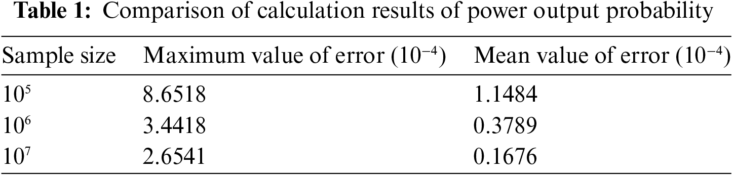
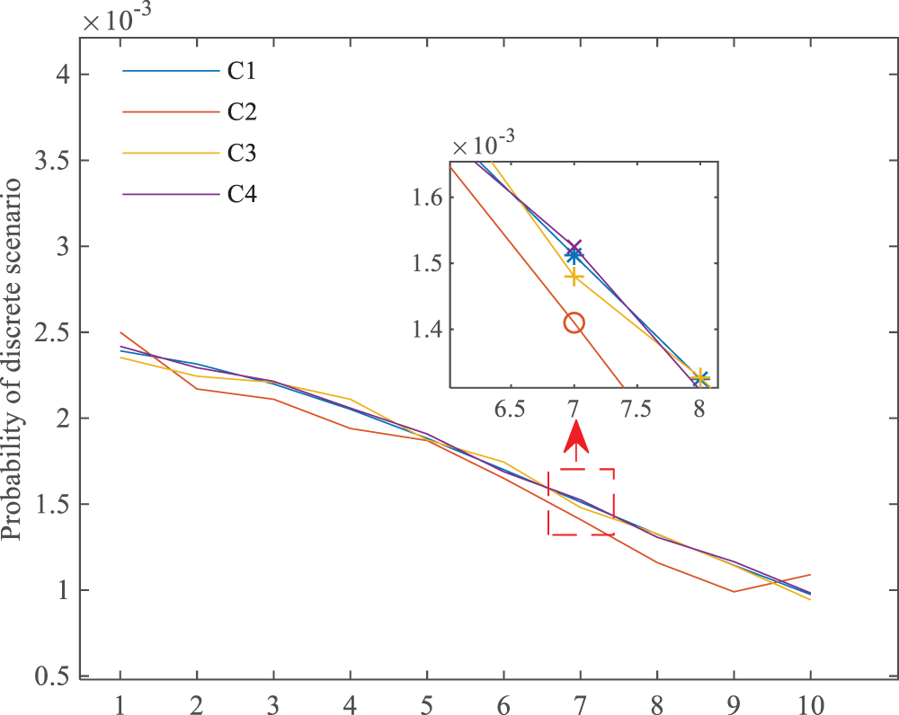
Figure 3: Comparison of probability calculations of wind power output scenarios

It can be observed from Table 1 that when the number of sampling times is 105, the magnitude of the maximum error is 10−4. As the number of random samples increases, both the maximum and average errors show a decreasing trend. It is worth noting that the increase in sample size enhances the accuracy of the proposed method’s calculations. The appropriate number of samples can be selected based on the accuracy requirements of the calculation results.

5.3 Performance Evaluation

The computational accuracy of the proposed method is validated using the IEEE 118-bus system, where the total system load is 22.71 MW + j17.04 Mvar, and the base power is 10 MVA. Wind farms with rated capacities of 6 MW and 4 MW are connected to buses 54 and 77, respectively. The wind speed correlation coefficient is 0.6, and the wind power penetration rate is 44.03% (10/22.71). Other data are provided in Section 5.1. The accuracy of the different methods is assessed by comparison with the results of 107 MCS. A comparison is made with the Correlated Cumulant Method (CCM) [19]. In this comparison, the CM handles correlation utilizing the Cholesky decomposition method. The accuracy of the power flow algorithm is evaluated using absolute percent error (APE) and (average root mean square) AMSR [20]. The analysis focuses on the calculation results of node 76 and branch 112–113, which are near the wind power connection point, as well as node 112 and branch 112–113, which are further away.

The results of the selected nodes and branches using the three PLF algorithms mentioned above are shown in Table 2. For both Bus 76 Voltage and Bus 112 Voltage, the mean values of the proposed method are extremely close to the MCS values, with very small relative errors (0.00112% and 0.00494%, respectively). The CCM method also provides close results but shows slightly larger relative errors (0.52000% for Bus 76 and 0.08932% for Bus 112). For Lines 52–53 Flow, the mean values of the Paper method are nearly identical to MCS with a low error of 0.00399%. However, the CCM method exhibits a much larger relative error of 0.98277%. Similarly, for Lines 112–113 Flow, the Paper method shows a very low error (0.00489%), while CCM has a significantly higher error (0.15642%). For all cases, the SDs for the proposed method are almost identical to the MCS, indicating accurate variability representation. The CCM method generally shows larger deviations for branch flows, indicating more variability or uncertainty in its calculations. It is apparent that the proposed method more accurate results for nodes significantly affected by wind power compared to the CCM, with results almost identical to those of the 107 MCS. Fig. 4 shows the CDFs for the corresponding nodes and branches. It can be seen that for nodes farther from the wind power nodes, both methods can accurately fit the probability curve of the state variables. However, the proposed method has a clear advantage in fitting the probability curves of the node voltage and branch active power for nodes closer to the wind power nodes.

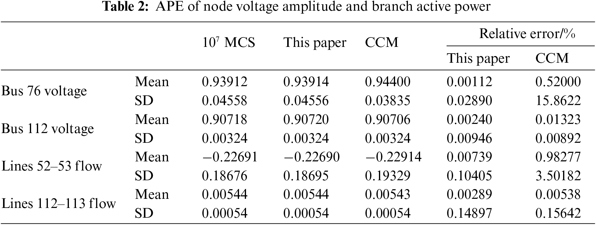
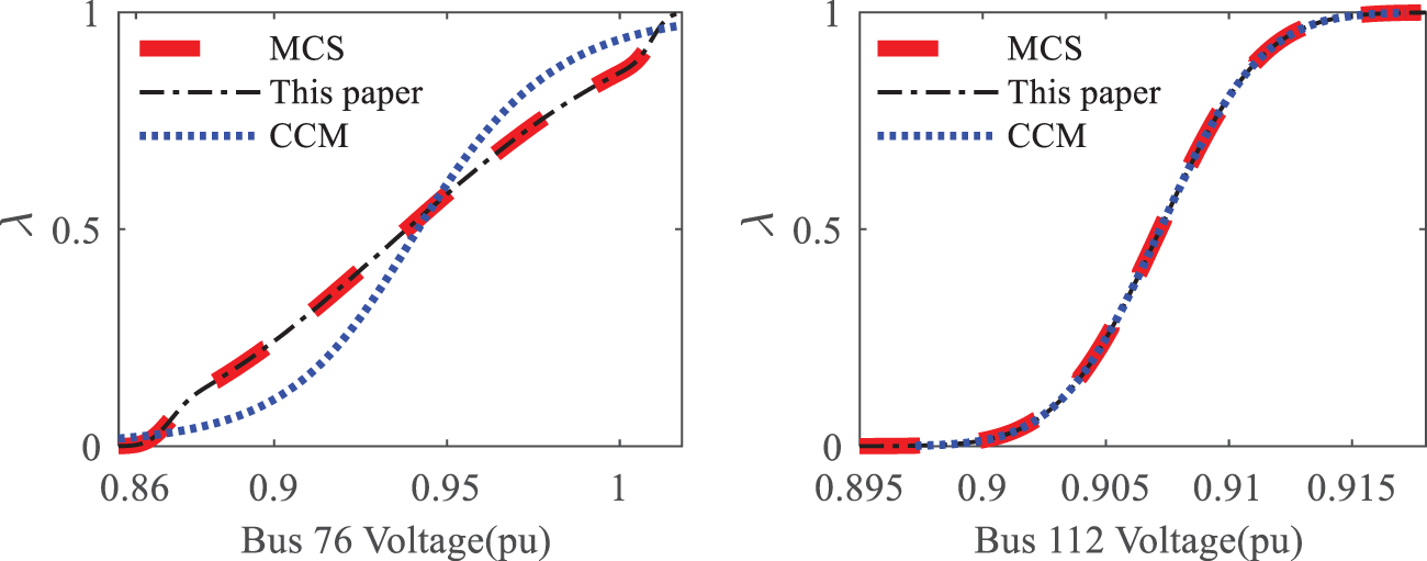
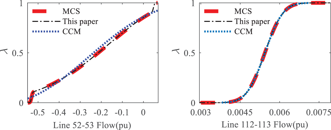
Figure 4: CDF curve of the output variable

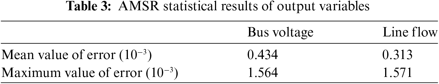
As shown in Table 3, the maximum value of the ARMS for node voltage is 1.564 × 10−3, and the average value is 4.34 × 10−4. The maximum value of the ARMS for branch active power is 1.571 × 10−3, and the average value is 3.13 × 10−4. The average error between node voltage amplitude and branch active power shall not exceed 4.34 × 10−4. The AMRS indicators of node 76 and branches 52–53, severely affected by wind, are 5.36 × 10−5 and 4.82 × 10−5, respectively. This method considers both the fitting accuracy of the probability curve and computational accuracy.

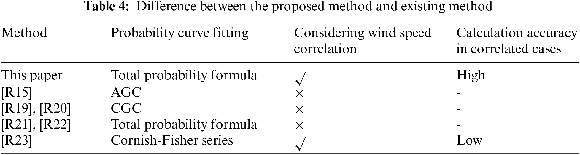
Through the analysis, it is evident that the proposed method has higher accuracy compared to the CCM. Table 4 presents the differences between the proposed method and existing studies.

5.4 Influence of Wind Speed Correlation on System Node Voltage

Connect nodes 18 and 17 of the IEEE 33-node system to wind farms with rated power of 600 and 400 kW, respectively, as shown in Fig. 5. The penetration rate of wind power is 1000/3715 = 26.92%. The data for the wind turbines and loads are shown in Section 5.1. The statistical characteristics of node voltage at node 15 were analyzed, and the results are shown in Figs. 6 and 7.

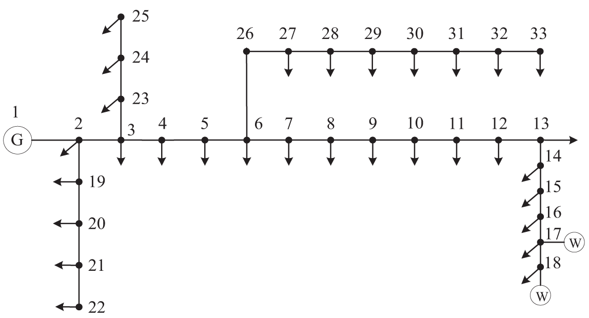
Figure 5: Improved IEEE33 node system

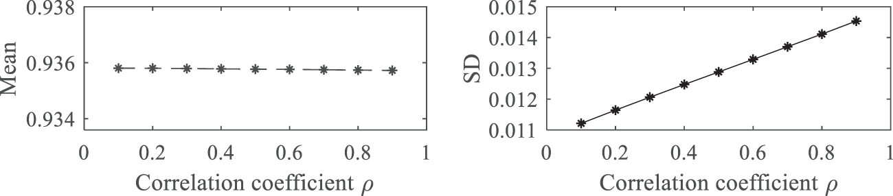
Figure 6: Correlation between voltage and wind speed at node 15

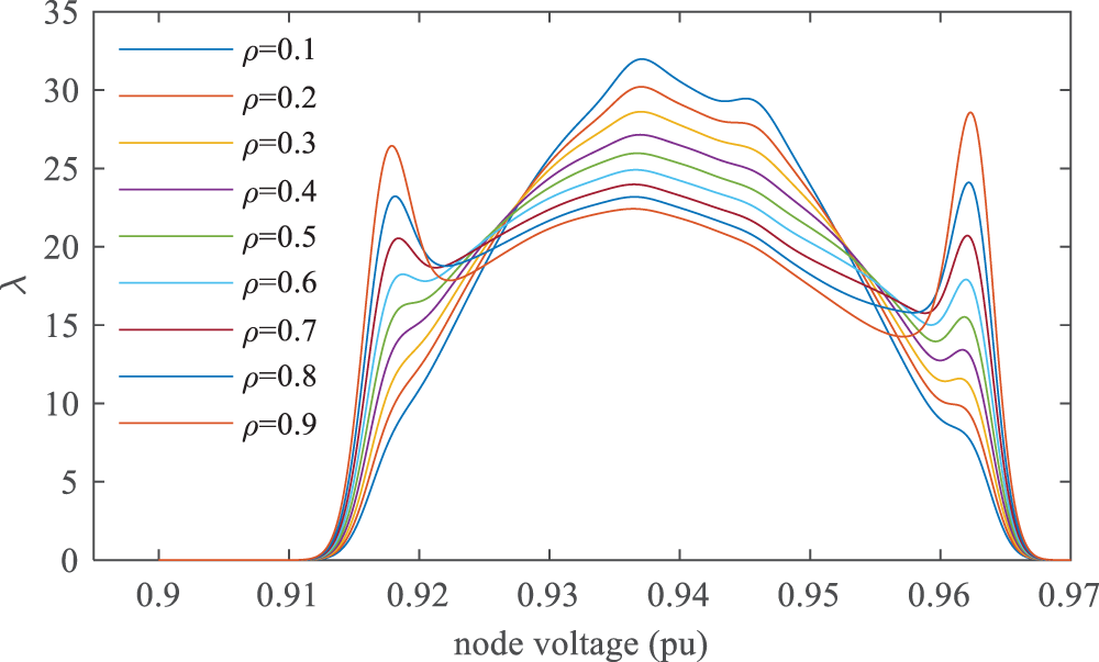
Figure 7: PDF curve of voltage at node 15

As shown in Fig. 6, the mean voltage of node 15 hardly changes with wind speed correlation, and the SD of node 15 voltage increases linearly with the wind speed correlation coefficient. It is evident from Fig. 7 that as the correlation increases, the probability of the low-voltage part and the high-voltage part of the node voltage increases, causing the voltage fluctuation to increase.

In the IEEE-33 node system, the distribution of voltage at node 15 was analyzed for wind farms with capacities of (200 kW, 300 kW), (400 kW, 600 kW), (600 kW, 900 kW), and (800 kW, 1200 kW) at nodes 17 and 18, respectively. The wind speed correlation coefficient is 0.8. The PDF curves of voltage at node 15 under scenarios of uncorrelated and correlated coefficients of 0.8 are shown in Fig. 8, and the results of mean and SD are shown in Table 5.

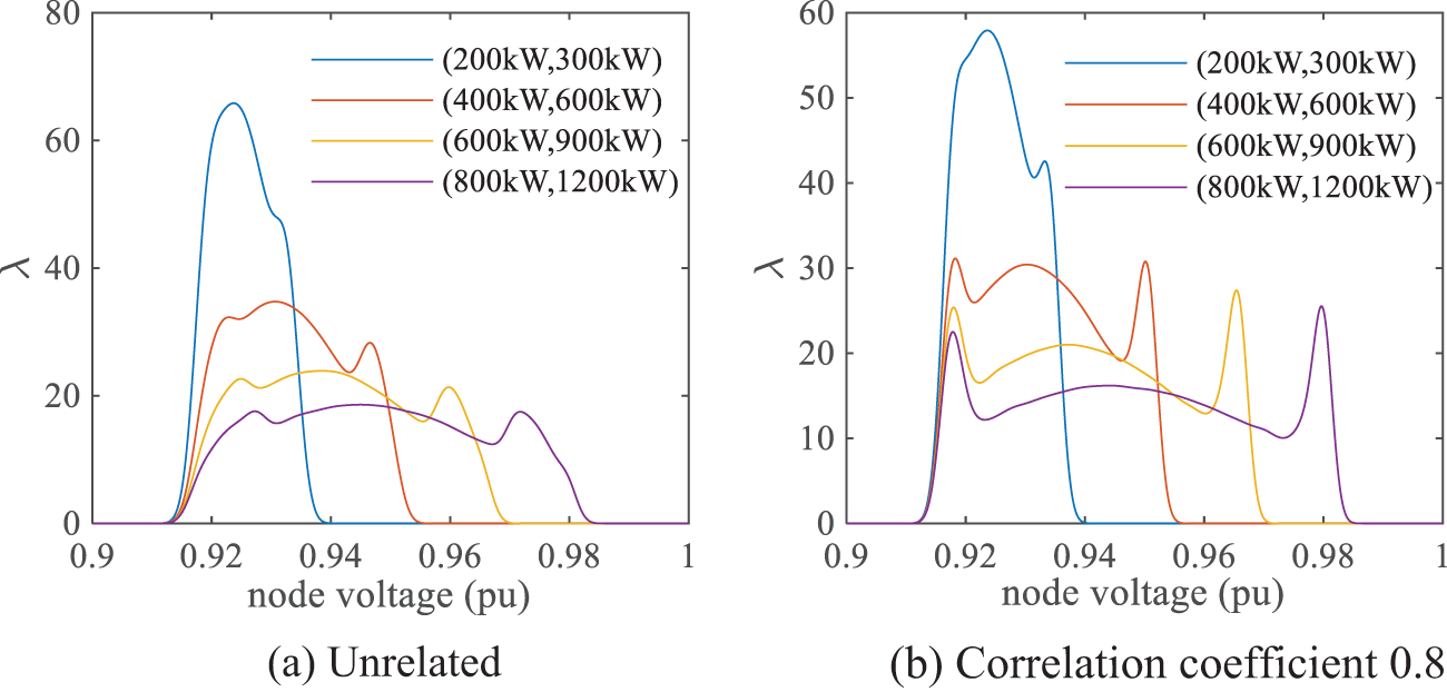
Figure 8: PDF curve of node 15 voltage at different wind power capacities

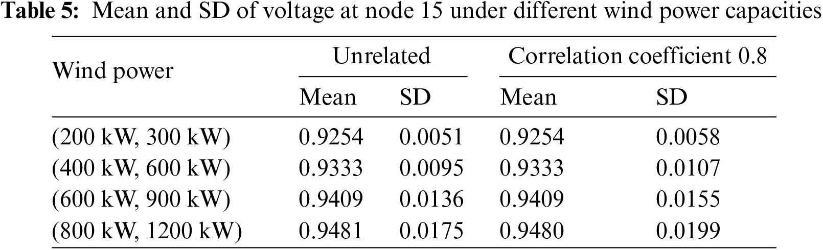
From Table 5, it is evident that as the wind power penetration rate grows, the expected value of the node voltage gradually rises. The SD of node voltage shows a positive correlation with the wind power penetration rate, which leads to an increase in the maximum node voltage and a higher probability of voltage limit violations. Fig. 8 visually demonstrates that as the wind power penetration rate gradually increases, the likelihood of high voltage, when considering correlation, is significantly higher than when correlation is not considered. Therefore, in integrating wind power into the power system, neglecting wind speed correlation under varying wind power penetration rates can result in an overly optimistic estimation of node voltage levels.

6  Conclusion

This paper proposes a method that combines random sampling and segmented discretization of wind farm power to solve the multi-scenario PLF calculation problem considering correlation. The important conclusions can be drawn as follows:

(1) Using random sampling to obtain the output probability of discrete scenarios in correlated scenarios solves the problem of difficulty in numerically calculating the output probability of discrete scenarios when wind speed is correlated. The errors in the probability calculations are all smaller than the order of 10−4.

(2) The proposed method can still ensure the computational accuracy of the segmented discretization method when dealing with correlation problems. Through case analysis, it is apparent that the calculation accuracy of the proposed method is nearly equivalent to that of 107 MCS. The relative errors of the node voltages and branch active power are all within 1%, and the AMSR values of the probability curves are all less than 1%.

(3) Analyze the operational characteristics of power systems under different degrees of wind speed correlation in IEEE 33 node systems. The SD of the voltage at node 14 increased by 29.6% when the correlation coefficient was 0.9 compared to when the correlation coefficient was 0.1. The results show that an increase in wind speed correlation will increase the probability of the node voltage PDF curve’s high and low voltage parts.

In addressing correlation issues, this paper only considers the correlation between wind farms and does not account for the correlation between wind power and load. In future work, we will address the issues of loads not following a normal distribution and the correlation between loads.

Acknowledgement: The authors would like to express our sincere appreciation to the anonymous referees for providing valuable suggestions and comments that have significantly contributed to the improvement of our manuscript.

Funding Statement: This research was supported by Basic Science Research Program through the National Natural Science Foundation of China (Grant No. 61867003).

Author Contributions: The authors confirm contribution to the paper as follows: study conception and design: Hongsheng Su, Xueqian Wang; data collection: Xueqian Wang; analysis and interpretation of results: Xueqian Wang, Hongsheng Su; draft manuscript preparation: Hongsheng Su, Xueqian Wang. All authors reviewed the results and approved the final version of the manuscript.

Availability of Data and Materials: The authors confirm that the data supporting the findings of this study is available within the article.

Ethics Approval: Not applicable.

Conflicts of Interest: The authors declare no conflicts of interest to report regarding the present study.

References

1. T. C. Zhang, J. X. Wang, G. Y. Li, M. Zhou, X. Y. Wang and Z. Liu, “Perception method of voltage spatial-temporal distribution of distribution network with high penetration of renewable energy,” (in ChineseAutom. Elect. Power Syst., vol. 45, no. 2, pp. 37–45, Jan. 2021. doi: 10.7500/AEPS20200430026. [Google Scholar] [CrossRef]

2. J. J. Xu, Z. J. Wu, Q. R. Hu, Y. Y. Xu, X. B. Dou and W. Gu, “Interval state estimation for active distribution networks considering uncertainties of multiple types of DGs and loads,” (in ChineseProc. CSEE, vol. 38, no. 11, pp. 3255–3266, Jun. 2018. doi: 10.13334/j.0258-8013.pcsee.170770. [Google Scholar] [CrossRef]

3. M. Y. Huang, Y. D. Fei, Z. N. Wei, Y. P. Zheng, G. Q. Sun and H. X. Zang, “Interval state estimation aided by forcasting for AC/DC distribution network with high proportion of renewable energy,” (in ChineseAutom. Elect. Power Syst., vol. 47, no. 16, pp. 34–43, Aug. 2023. doi: 10.7500/AEPS20220804001. [Google Scholar] [CrossRef]

4. M. Aien, M. Fotuhi-Firuzabad, and M. Rashidinejad, “Probabilistic optimal power flow in correlated hybrid wind-photovoltaic power systems,” IEEE Trans. Smart Grid, vol. 5, no. 1, pp. 130–138, Jan. 2014. doi: 10.1109/TSG.2013.2293352. [Google Scholar] [CrossRef]

5. C. J. Xia, X. T. Zheng, L. Guan, and S. Baig, “Probability analysis of steady-state voltage stability considering correlated stochastic variables,” Int. J. Electr. Power Energy Syst., vol. 131, no. 12, May 2021, Art. no. 107105. doi: 10.1016/j.ijepes.2021.107105. [Google Scholar] [CrossRef]

6. Y. Chen, M. Chen, Z. Tian, and Y. Liu, “Voltage unbalance management for high-speed railway considering the impact of large-scale DFIG-based wind farm,” IEEE Trans. Power Deliv., vol. 35, no. 4, pp. 1667–1677, Aug. 2020. doi: 10.1109/TPWRD.2019.2949563. [Google Scholar] [CrossRef]

7. X. L. Chen, J. Han, T. T. Zheng, P. Zhang, S. M. Duan and S. H. Miao, “A vine-copula based voltage state assessment with wind power integration,” Energies, vol. 12, no. 10, May 2019, Art. no. 2019. doi: 10.3390/en12102019. [Google Scholar] [CrossRef]

8. R. Taghavi, H. Samet, A. R. Seifi, and Z. M. Ali, “Stochastic optimal power flow in hybrid power system using reduced-discrete point estimation method and latin hypercube sampling,” IEEE Canadi J. Electr. Comput. Eng., vol. 45, no. 1, pp. 63–67, 2022. doi: 10.1109/ICJECE.2021.3123091. [Google Scholar] [CrossRef]

9. C. S. Saunders, “Point estimate method addressing correlated wind power for probabilistic optimal power flow,” IEEE Trans. Power Syst., vol. 29, no. 3, pp. 1045–1054, May 2014. doi: 10.1109/TPWRS.2013.2288701. [Google Scholar] [CrossRef]

10. A. R. Nezhad, G. Mokhtari, M. Davari, A. R. Araghi, S. H. Hosseinian and G. B. Gharehpetian, “A new high accuracy method for calculation of LMP as a random variable,” in 2009 Int. Conf. Electr. Power Energy Convers. Syst., Sharjah, United Arab Emirates, 2009, pp. 1–5. [Google Scholar]

11. V. Singh, T. Moger, and D. Jena, “Probabilistic load flow approach combining cumulant method and k-means clustering to handle large fluctuations of stochastic variables,” IEEE Trans. Ind. Appl., vol. 59, no. 3, pp. 2832–2841, May–Jun. 2023. doi: 10.1109/TIA.2023.3239558. [Google Scholar] [CrossRef]

12. Y. M. Zhang et al., “Electric vehicle charging station planning strategy based on probabilistic power flow calculation of distribution network,” (in ChinesePower Syst. Prot. Control, vol. 47, no. 22, pp. 9–16, Nov. 2019. doi: 10.19783/j.cnki.pspc.181532. [Google Scholar] [CrossRef]

13. V. Singh, T. Moger, and D. Jena, “Probabilistic load flow for wind integrated power system considering node power uncertainties and random branch outages,” IEEE Trans. Sustain. Energy, vol. 14, no. 1, pp. 482–489, Jan. 2023. doi: 10.1109/TSTE.2022.3216914. [Google Scholar] [CrossRef]

14. B. Chen, Z. Y. Li, S. P. Li, Q. Z. Zhao, and X. D. Liu, “A wind power prediction framework for distributed power grids,” Energy Eng., vol. 121, no. 5, pp. 1291–1307, May 2024. doi: 10.32604/ee.2024.046374. [Google Scholar] [CrossRef]

15. X. Y. Zhu, W. X. Liu, and J. H. Zhang, “Probabilistic load flow method considering large-scale wind power integration,” (in ChineseProc. CSEE, vol. 33, no. 7, pp. 77–85, Mar. 2013. doi: 10.19783/j.cnki.pspc.181532. [Google Scholar] [CrossRef]

16. R. Cao, J. Xing, B. Sui, and H. Ma, “An improved integrated cumulant method by probability distribution pre-identification in power system with wind generation,” IEEE Access, vol. 9, pp. 107589–107599, Jul. 2021. doi: 10.1109/ACCESS.2021.3100627. [Google Scholar] [CrossRef]

17. Y. H. Gao and C. Wang, “Probabilistic load flow calculation of distribution system including wind farms based on total probability formula,” (in ChineseProc. CSEE, vol. 35, no. 2, pp. 327–334, Jan. 2015. doi: 10.13334/j.0258-8013.pcsee.2015.02.009. [Google Scholar] [CrossRef]

18. L. Ye, Y. L. Zhang, C. H. Zhang, P. Lu, Y. N. Zhao and B. Y. He, “Combined Gaussian mixture model and cumulants for probabilistic power flow calculation of integrated wind power network,” Comput. Electr. Eng., vol. 74, no. 1, pp. 117–129, Mar. 2019. doi: 10.1016/j.compeleceng.2019.01.010. [Google Scholar] [CrossRef]

19. D. Y. Shi, D. F. Cai, J. F. Chen, X. Z. Duan, H. J. Li and M. Q. Yao, “Probabilistic load flow calculation based on cumulant method considering correlation between input variables,” Proc. CSEE, vol. 32, no. 28, pp. 104–113, Oct. 2012. doi: 10.13334/j.0258-8013.pcsee.2012.28.014. [Google Scholar] [CrossRef]

20. C. X. Wang, C. X. Liu, F. Tang, D. C. Liu, and Y. X. Zhou, “A scenario-based analytical method for probabilistic load flow analysis,” Elect. Power Syst. Res., vol. 181, no. 3, Mar. 2020, Art. no. 106193. doi: 10.1016/j.epsr.2019.106193. [Google Scholar] [CrossRef]