Reactive Power Optimization Model of Active Distribution Network with New Energy and Electric Vehicles

1  Introduction

The rapid development of electric vehicles and new energy technologies has played an important role in alleviating the energy crisis and achieving the “double carbon” goal in China [1,2]. However, the fluctuation of new energy and the real-time change of load lead to the reactive power optimization of the distribution network, which is actually a dynamic process [3]. Compared with static reactive power optimization, it not only increases the number of variables with the refinement of the time scale but also makes the dynamic reactive power optimization problem have space-time coupling characteristics due to the coupling of dynamic constraints and static constraints between discrete variables [4].

How to deal with dynamic constraints reasonably is the difficulty of solving dynamic reactive power optimization problems. The common strategy is to decouple the original problem in time and space so as to transform it into a static reactive power optimization problem [5,6]. In Reference [7], the electric vehicle charging station is used as the reactive power compensation source, which effectively improves the voltage quality and system stability. However, there are many reactive power decisions, and there is a complex space-time coupling between variables, which makes the model difficult to solve. Reference [8] decouples the dynamic reactive power optimization problem in time and space and formulates the action schedule of reactive power regulation equipment through heuristic strategy and reactive power compensation error, so as to transform the dynamic reactive power optimization problem into multiple static reactive power optimization problems. Based on the day-ahead load forecasting curve, the literature [9–11] classifies the predicted power of each period by mathematical statistics, so as to obtain the action time of the reactive power compensation device and perform static reactive power optimization in the classified period. The literature [12] adopts a two-stage reactive power optimization method. In the first stage, the discrete reactive power compensation amount is optimized, and then the input amount is fixed, and the continuous reactive power compensation device is used to correct it under the condition of meeting the limit of its action times. The above research has certain reference significance for the exploration of space-time decoupling methods, but the influence of source-load uncertainty on space-time decoupling is not considered.

Furthermore, the reactive power optimization problem after space-time decoupling is essentially a large-scale nonlinear mixed integer problem, and the existence of a large number of discrete variables makes it difficult to solve the model. In this regard, References [13,14] used the decomposition coordination method to coordinate discrete variables and continuous variables. This method reduces the difficulty of solving to a certain extent, but solving the two variable types independently will lead to search path offset and reduce the global optimization ability of the algorithm. Reference [15] used particle swarm optimization to optimize discrete variables and continuous variables, respectively, and then used the results of each optimization as the initial value for alternating iterative optimization. This method effectively separates discrete variables and continuous variables and reduces the difficulty of solving. However, solving discrete variables by particle swarm optimization will change the search direction, and it is difficult to obtain the global optimum. In the later stage of convergence, species diversity decreases, and it is easy to fall into a local optimum. The artificial hummingbird algorithm (AHA) is proposed in [16], which has high search accuracy, fast convergence speed, and a simple principle. However, in the later stage of optimization, the diversity of samples is reduced, and it is easy to fall into a local optimum.

Based on the above analysis, this paper takes into account the uncertainty of electric vehicles, new energy, and residential electricity load and proposes a time-space decoupling strategy for dynamic reactive power optimization. The strategy comprehensively considers the influence of new energy output, electric vehicle charging load, and residential electricity load fluctuation. The k-medoids clustering algorithm is used to divide the reduced scene into periods, and then the static reactive power optimization is carried out for each period, so as to decouple the original problem in time and space. Aiming at the characteristics of the model after space-time decoupling, a hybrid optimization algorithm combining the improved artificial hummingbird algorithm (TAMAHA) and genetic algorithm is designed. Based on the principle of cross feedback, the algorithm solves the continuous variables and discrete variables differently, thereby reducing the difficulty of solving and improving the operating indicators of the system.

2  Dynamic Reactive Power Optimization Model

2.1 Objective Function

The model proposed in this paper adopts the method of spatiotemporal decoupling, which changes the goal of the total network loss, voltage offset and voltage stability index of the whole day to the goal of the minimum index of each hour, and then replaces the dynamic reactive power optimization with static reactive power optimization.

1) Minimum network loss

f1=min∑s=1Nsπw(s)∑i=1N∑j∈ϕireal(1Yij)⋅Pij,s2+Qij,s2Uij,s2(1)

In the formula, Ns-number of scenes; πw(s)-probability of occurrence of scenario s; N-number of nodes; Yij-branch admittance; Pij,s, Qij,s-active and reactive power flowing from the first end of branch ij in scenario s; Uij,s-voltage at the first end of branch ij in scenario s; ϕi-the set of nodes connecting node i; real()-take the real part operation.

2) The node voltage offset is minimum

f2=min∑s=1Nsπw(s)∑i=1N(Ui,s−Ui,nUi,max−Ui,min)2(2)

In the formula, Ui,s is the voltage amplitude of node i under scenario s; Ui,max, Ui,min and Ui,n represent the upper, lower and rated voltage of node i, respectively.

3) Optimal system stability [17]

f3=minl∈ij∑s=1Nsπw(s)⋅(4(XijPij,s−RijQij,s)2+XijQij,s+RijPij,s)(3)

In the formula, Rij, Xij-branch ij resistance, reactance; l-branch set; system collapse when f3≥1.

The dimensions of each subobjective are different, so it is necessary to normalize them and then establish a single objective function.

fk∗={1,fk≤fk,minfk−fk,minfk,max−fk,min,fk,min<fk<fk,max0,fk≥fk,max(4)

F=w1f1∗+w2f2∗+w3f3∗(5)

In the formula, fk∗-the specific value of the normalized k of the sub-objective, in which k=1,2,3; fk,min, fk,max-single objective optimization and pre-optimization results; w1, w2, w3-weight coefficient, and w1+w2+w3=1; F-normalized objective function value, the closer to 0, the better the reactive power optimization result.

Analytic hierarchy process [18] was used to determine the weight coefficient, and the judgment matrix was constructed according to the importance degree: active power loss > voltage offset > system stability:

A=(1351/3131/51/31)(6)

It can be obtained by calculation w1 = 0.6370, w2 = 0.2583, w3 = 0.1047.

2.2 Constraints

It should be stated that the following constraints are applicable to any scenario, and then a specified scenario is no longer described, so the subscript s representing a certain scene is omitted.

1) Power balance constraints

{Pgrid,j+∑j∈πWTPWT,j+∑j∈πPVPPV,j=∑j∈πLPLoad,j+∑j∈πEVSPEVS,j+∑j∈πlPl,jQgrid,j+∑j∈πWTQWT,j+∑j∈πPVQPV,j+∑j∈πCBQCB,j=∑j∈πLQLoad,j+∑j∈πlQl,j(7)

In the formula, Pgrid,j, PWT,j, PPV,j are the active power of the large power grid injected into node j, the active power of wind power and photovoltaic, and Load, PLoad,j, PEVS,j, Pl,j are the active power of the load consumed at node j, the charging power and active power loss of the electric vehicle charging station. Qgrid,j, QWT,j, QPV,j are the reactive power, wind power and photovoltaic reactive power of the large power grid injected into node j, QLoad,j, Ql,j are the reactive power and reactive power loss of load at node j, respectively, and πWT, πPV, πCB and πEV are the node set of installed fan, photovoltaic, switchable capacitor bank and electric vehicle charging station.

2) Voltage and current constraints

{Iij,min≤Iij≤Iij,maxUi,min≤Ui≤Ui,max(8)

In the formula, Iij,max, Iij,min-the upper and lower limits of the current flowing through the branch ij.

3) Control variable constraints

{QPW,jmin≤QPW,j≤QPW,jmaxQPV,jmin≤QPV,j≤QPV,jmax0≤NC≤NC,maxQSVC,jmin≤QSVC,j≤QSVC,jmax(9)

In the formula, QPW,jmax, QPW,jmin, are the upper and lower limits of the fan reactive power output of the connecting node j, respectively; QPV,jmax, and QPV,jmin are the upper and lower limits of the photovoltaic reactive power output of the connected node j, and NC,max is the maximum number of capacitor bank switching of the connected node j; QSVC,jmin, and QSVC,jmax are the upper and lower limits of SVC reactive power compensation for connecting nodes j, respectively.

4) Power constraints of EV charging stations

PEVS,jmin≤PEVS,j≤PEVS,jmax(10)

QEVS,jmin≤QEVS,j≤QEVS,jmax(11)

(PEVS,j)2+(PEVS,j)2≤SEVS,j(12)

In the formula, PEVS,jmin, PEVS,jmax -the minimum and maximum active power consumed at node j; QEVS,j,tmin, QEVS,j,tmax-the minimum and maximum reactive power injected at node j; SEVS,j,t-the capacity of the charging station at node j.

5) Constraints on the number of CB movements

∑t=124Cj,t⊕Cj,t−1≤nc(13)

In the formula, the number of input groups of the capacitor bank at node j at Cj,t-t time; The ⊕-XOR operator; nc-the maximum number of times a day can be switched, take 8 times. It should be noted that this paper considers that each adjustment of the capacitor bank is an action.

3  Clustering, Local Relaxation-Correction Reactive Power Optimization Decoupling Strategy

The objective function of dynamic reactive power optimization is the minimum sum of all indexes in all hours of a day. Considering the existence of discrete variable dynamic bundle reduction, this paper first divides the time period by clustering algorithm, establishes the action schedule of capacitor banks, and then determines the input number of capacitor banks in each time period by local relaxation, finally, the reactive power compensation device with continuous adjustment ability can be flexibly controlled to achieve dynamic reactive power optimization.

3.1 Clustering

The fluctuation of active power output of new energy, mainly wind power and photovoltaic, residential electricity load and electric vehicle charging load is the main reason for the different operating states of distribution network in each hour, so it is more reasonable to cluster their power.

First of all, the whole day is divided into 24 time periods, each time period is 1 h, and the expected active power of wind power and photovoltaic power, the expected electricity load of residents and the expected charging load of EV charging stations in each hour period are taken as the main factors affecting the clustering results. The power sequence of the whole day can be expressed as follows:

{PWT,aav=(PWT,a,1av,PWT,a,2av,⋯PWT,a,Tav,⋯,PWT,a,24av),a=1,2,⋯,APPV,bav=(PPV,b,1av,PPV,b,2av,⋯PPV,b,Tav,⋯,PPV,b,24av),b=1,2,⋯,BPEVS,dav=(PEVS,d,1av,PEVS,d,2av,⋯PEVS,d,Tav,⋯,PEVS,d,24av),d=1,2,⋯,DPLoadav=(PLoad,1av,PLoad,2av,⋯PLoad,Tav,⋯,PLoad,24av)(14)

{PWT,a,Tav=∑s=1Nsπw(s)⋅PWT,s,a,TPPV,b,Tav=∑s=1Nsπw(s)⋅PPV,s,b,TPEVS,d,Tav=∑s=1Nsπw(s)⋅PEVS,s,d,TPLoad,Tav=∑s=1Nsπw(s)⋅PEVS,s,T(15)

Among them,PWT,,s,a,T, PPV,s,b,T are the active output of wind turbine a and photovoltaic power station b respectively under scenario s in time period T; PLoad,s,T is the residential power load under scenario s during the time period T; PEVS,s,d,T refers to the charging load of EV charging station d under scenario s in time period T; A, B, D, respectively, the number of wind turbines, photovoltaic power stations and electric vehicle charging stations; PWT,a,Tav, PPV,b,Tav, PEVS,d,Tav PLoad,Tav is the expected active power of wind turbine a, photovoltaic station b, electric vehicle charging station d and load during the period T, in turn.

Further, the wind power, photovoltaic active power output, residential power load and charging load of EV charging stations in each hour segment are classified into A sample point with dimension A+B+D+1, whose expression is as follows:

xT=[PPW,1,Tav,PPW,2,Tav,⋯,PPW,A,Tav,PPV,1,Tav,PPV,2,Tav,⋯,PPV,B,Tav,PLoad,tavPEVS,1,Tav,PEVS,2,Tav,⋯,PEVS,D,Tav](T=1,2,⋯24)(16)

In the formula, xT is the data of the T sample point.

Secondly, k-medoids algorithm is used to cluster the samples. The specific operation is as follows:

i) k sample points are selected as the center of mass.

ii) Calculate the Euclidean distance from the sample point to the center of mass. The closer the sample point is, the higher the similarity between the tabular data is. The calculation formula is as follows:

d(xT,cr)=sqrt(∑a=1A(PPW,a,Tav−PPW,a,rav)2+∑b=1B(PPV,b,Tav−PPV,b,rav)2+∑d=1D(PEVS,d,Tav−PPW,d,rav)2+(PLoad,Tav−PPW,rav)2),(r=1,2,⋯,k)(17)

where cr is the RTH cluster center and sqrt represents the root operation. After the distance calculation is completed, the sample points closest to the center of mass are classified as the cluster where the center of mass is located.

iii) Take each point in the cluster as the center of mass, calculate the total distance between the other points in the cluster and the center of mass, and then select the point with the smallest total distance as the new center of mass.

iv) Repeat steps ii) and iii) until the position of the center of mass does not change. After the clustering is completed, all sample points are classified into corresponding clusters.

Finally, the samples of adjacent time periods in the same cluster are combined into one period, and the combined period is the action time period of the capacitor bank. When reactive power is optimized, the input times of the capacitor bank in each period after the merger are fixed, and the input quantity of the capacitor bank in different time periods can be different. If the combined time period L it is greater than the maximum number of capacitor bank switching times nc, then the secondary segmentation is carried out, the specific operation is: to calculate the Euclidean distance between the sample points of adjacent time periods after the segmentation, and sort the distance from small to small, and then merge the adjacent time intervals according to this order until L≤nc.

3.2 Local Relaxation

In the allotted time period, the maximum number of switching times of the relaxed capacitor bank is constrained, which is regarded as a continuous variable, and static reactive power optimization is carried out in the time section of the hour level, and the relaxation solution of the hourly reactive power compensation capacity of the capacitor bank is obtained:

QC=[Q1Q2⋯QT⋯Q24](18)

In the formula, QC is the reactive power compensation sequence of the capacitor bank after relaxation; Qi is the reactive power compensation amount of the capacitor bank in the i hour segment.

The average value of the reactive power compensation amount of the capacitor bank input in each time period is taken as the reactive power input amount of all hours in the time period, and then it is normalized, and the normalization result is the final input amount of the capacitor group:

QC∗=[Q1¯Q1¯⋯Q1¯⏞g1,|Q2¯Q2¯⋯Q2¯⏞g2,|⋯|,QL¯QL¯⋯QL¯⏞gL](19)

In the formula, QC∗ is the final reactive power compensation sequence of the capacitor bank; Qi¯ is the reactive power compensation amount of capacitor group in each i hour segment in time period i; gi indicates the number of hours contained in time period i.

3.3 Calibration

Finally, on the basis of the optimization of discrete variables, continuous variables are used for correction: the reactive power output of wind turbine, photovoltaic power station, electric vehicle charging station and SVC is used as the decision variable for static reactive power optimization in the second stage, and the optimization result is the final solution of continuous variables. At this point, all decision variables have been optimized.

4  Hybrid Optimization Algorithm

The reactive power optimization model after spatiotemporal decoupling involves a large number of continuous and discrete variables, which makes the solution of the model more complicated. A hybrid optimization algorithm combining the improved artificial hummingbird algorithm and genetic algorithm is proposed to solve the model in this paper. Based on the cross-feedback mechanism, the two types of variables are solved independently. Then the optimization result is fed back to another algorithm as the initial value, which not only reduces the variable complexity, but also effectively combines the advantages of each optimization algorithm to deal with different optimization variables, so that the algorithm’s solving speed and global search ability are greatly improved.

4.1 Improved Artificial Hummingbird Algorithm

The AHA algorithm simulates the flight skills and foraging strategies of hummingbirds in nature. Three flight skill models, namely, axial flight, diagonal flight and omnidirectional flight, and three foraging behavior models, namely, guided foraging, regional foraging and migratory foraging, were established, and the memory function of the access table model was constructed. The existence of the access table prevents individuals from frequently searching for food sources that have already been visited, thus speeding up the collection. However, the AHA algorithm tends to fall into local optimality due to low species diversity in the later stages of population initialization and optimization. In this regard, this paper improves the AHA algorithm, the specific steps are as follows:

In this regard, this paper improves the AHA algorithm, the specific steps are as follows:

(1) Tent Chaotic map initialization population [19]:

ym+1={ymα,0≤ym≤α1−ym1−α,α≤ym≤1(20)

α is 0.5, and the steps of chaos perturbation are:

The chaos variable y is generated according to Eq. (20).

Map chaos variables to the solution space.

Y=xmin+(xmax−xmin)⋅y(21)

In the formula, xmin,xmax-variable upper and lower limits.

a) Chaotic disturbance.

Xnew′=(X′+Y)/2(22)

In the formula, Xnew′-individual after disturbance; X′-disturbed individuals; Y-the amount of disturbance.

(2) An adaptive mutation operator based on population aggregation was introduced to enhance the diversity of the population. Population aggregation C is defined as:

C=∑k=1D∑i=1NP|Xi,k−Xk¯|(23)

In the formula, D-individual dimension; NP-Individual number; Xi,k-the k-dimensional position of individual i.

Population aggregation degree C reflects the richness of population diversity, and the larger the population, the more dispersed the individuals and the more abundant the species. Based on Eq. (23), an adaptive mutation operator is introduced:

u=Xbest,j+F(Xr1,j−Xr2,j)(24)

v=Xr3,K+F(Xr5,K−Xr5,j)(25)

Vi,j=C×u+(1−C)×v(26)

In the formula, F∈[0,1]-Shrinkage factor; i,r1∼r5-[1,NP] random numbers on, and not equal to each other; j,K∈[1,D], and K≠j; K-For the heterodimensional dimensions selected by random generalized method.

(3) After the adaptive variation strategy was added, some hummingbirds after location update performed cross-selection operations according to Eqs. (27) and (28).

Ui,jt={Vi,jt,if rand<CRXi,jt, else(27)

Xit+1={Uit,iffit(Uit)>fit(Xit)Xit, else(28)

In the formula, Ui,j-the dimension j of individual i is changed into position; t-number of iterations; CR-cross probability.

4.2 Cross-Feedback Hybrid Optimization Algorithm

In the local relaxation reactive power optimization stage, the continuous and discrete variables are solved by TAMAHA algorithm and GA algorithm respectively. Genetic algorithm adopts binary coding method, which has unique advantages in solving optimization problems involving discrete variables. The cross-feedback mechanism of the proposed hybrid optimization algorithm is as follows: different algorithms are used to independently solve different types of variables, chaotic initialization of discrete variable X and continuous variable Y at the initial stage, optimization of variable X by GA algorithm under the condition that Y remains fixed, and then the optimization result of X is fed back to variable Y as initial value. On this basis, the TAMAHA algorithm is used to optimize the variable Y, and then X is optimized on the basis of the optimization results of the variable Y, so the cross-feedback is optimized until the termination condition is met. The algorithm flow is shown in Fig. 1.

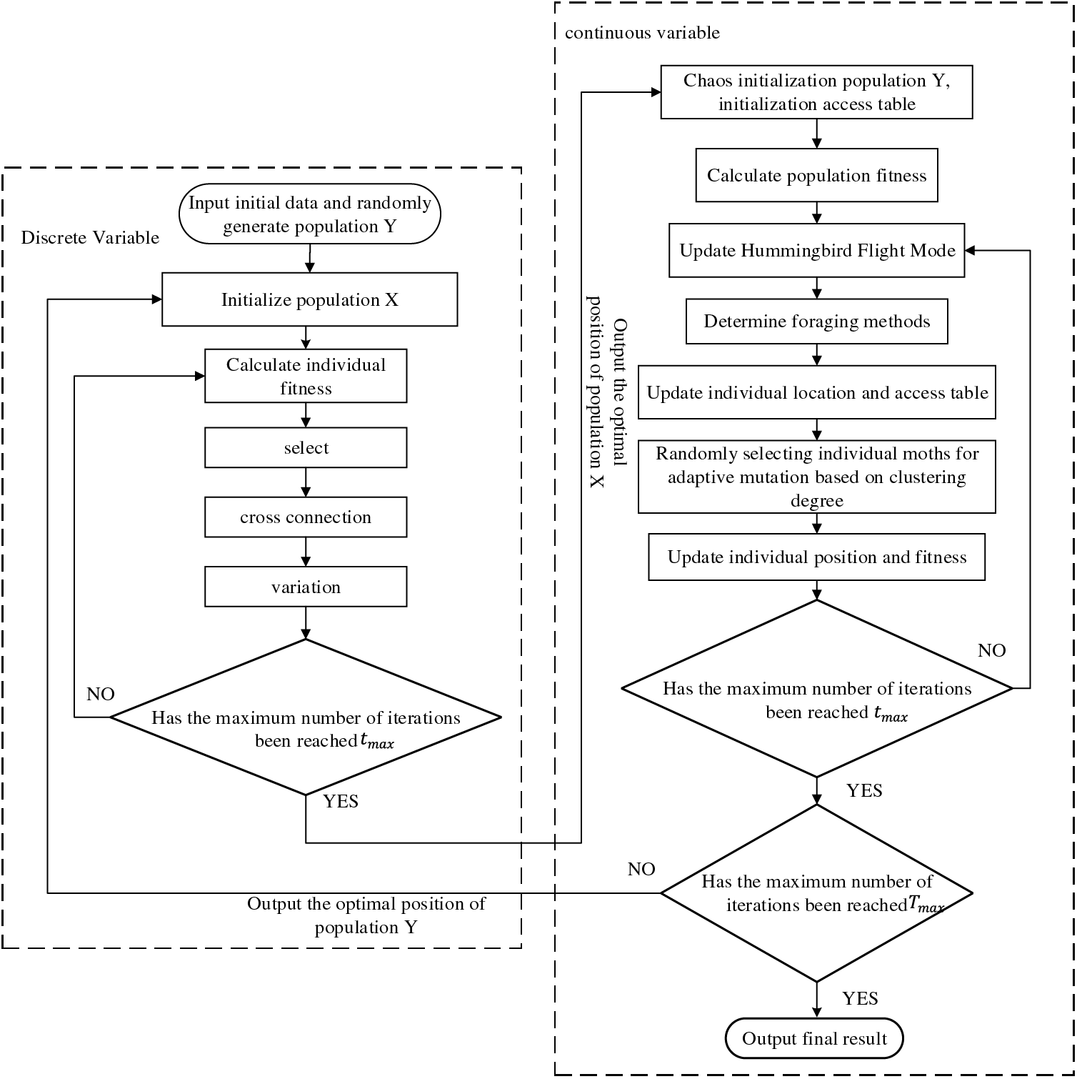
Figure 1: Algorithm procedure

5  Analysis of Numerical Examples

5.1 Setting Basic Parameters

To improve the IEEE33-node system for analysis, as shown in Fig. 2. The reference capacity is 10 MW and the voltage level is 12.66 kV. Wind power generator (WT) access node 17, capacity 1.2 MW, power factor between −0.95 and 0.95 continuously adjustable; Photovoltaic power station (PV) access node 33, rated capacity of 1 MW, PV inverter capacity of 1.1 times the rated capacity; Capacitor bank SCB1 and SCB2 are connected to 9 and 32 nodes, respectively, and each group has 10 groups of 100 kvar. The SVC can connect 5, 24, and 28 nodes with a capacity of 800 kvar. Electric vehicle charging stations (EVS) are connected to 12 and 22 nodes, and centralized converters are selected to connect to the grid, with a maximum apparent capacity of 0.8 MVA. The standard deviation of load, wind speed and light intensity is 5%, 10% and 10% of the predicted value. The LHS sampling value is 1000, and the reduced scenario Ns=5. Figs. 3–5 show the output scenarios of wind power, photovoltaic power and load after scenario reduction, and Fig. 6 shows the probability of occurrence of corresponding scenarios. Set the population size of the TAMAHA algorithm as N=30, the hummingbirds performing adaptive variation as 20% of the population, the crossover probability as 0.9, the reduction factor as 0.5, the maximum iteration number tmax=30, t, and the maximum iteration number of cross feedback Tmax=100, the parameters of genetic algorithm are shown in the paper [20].

Figure 2: Modified IEEE33-node system diagram

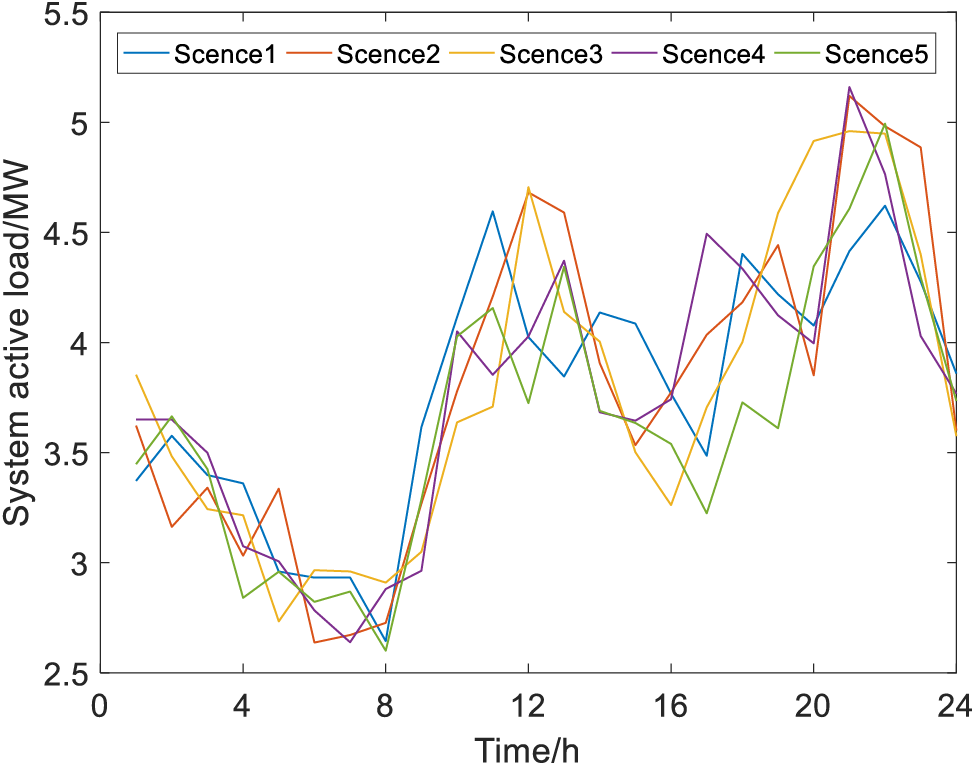
Figure 3: Wind power scene

Figure 4: Photovoltaic output scenario

Figure 5: Active load scenario

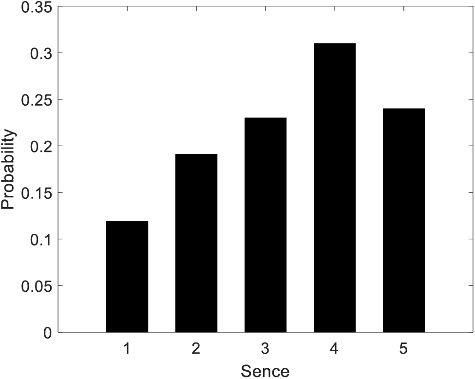
Figure 6: Scene occurrence probability

Assume that the proportion of electric private cars, electric business cars and electric taxis in EVS1 charging station at node 12 is 0.77, 0.1 and 0.13, and that at node 22 EVS2 charging station, the proportion is 0.69, 0.22 and 0.09, with a total of 400. For specific parameters, refer to the reference [21]. Monte Carlo method was used for prediction, as shown in Fig. 7. Fig. 7 shows the forecast value of hourly residential electricity load and total load the next day.

Figure 7: Electric vehicle charging load

5.2 Analysis of Space-Time Decoupling Strategy

In order to verify the effectiveness of the spatio-temporal decoupling strategy proposed in this paper, firstly, the k-medoids clustering algorithm is used to cluster the residential electricity load, electric vehicle charging load and new energy output. The elbow method is used to determine the number of clusters to be 4, and the results are shown in Fig. 8. According to the calculation, the 24 h of a day is divided into five sections: 01:00–09:00, 10:00–11:00, 12:00–13:00, 14:00–17:00, 18:00–24:00, as shown in Table 1.

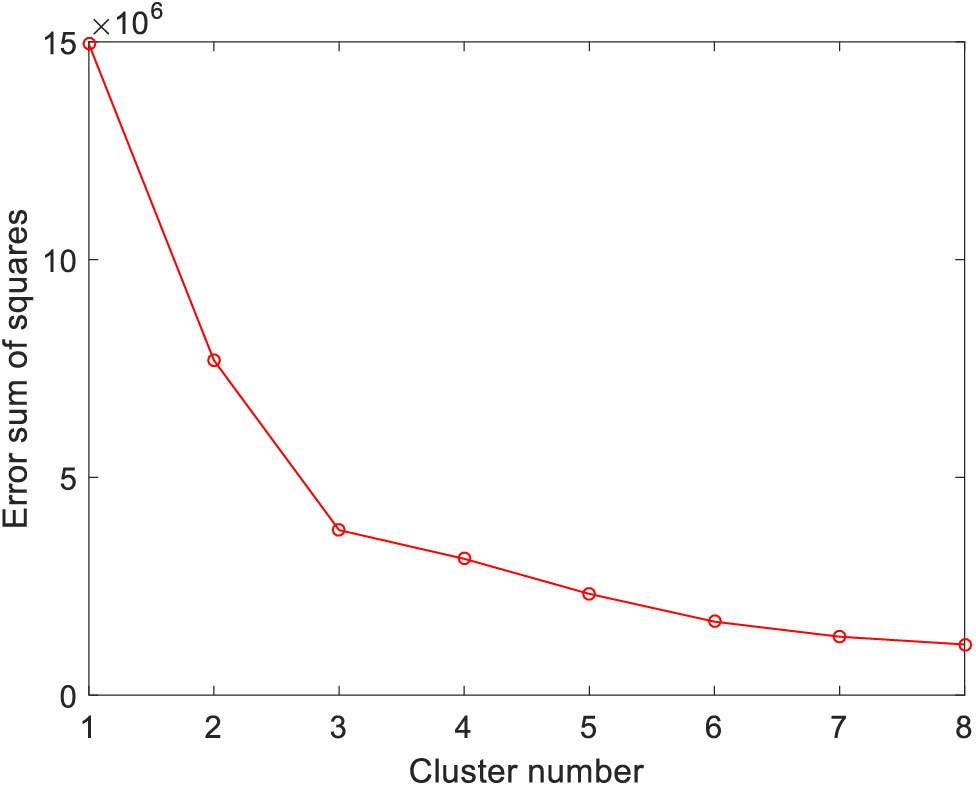
Figure 8: Different K-value clustering deviation graph

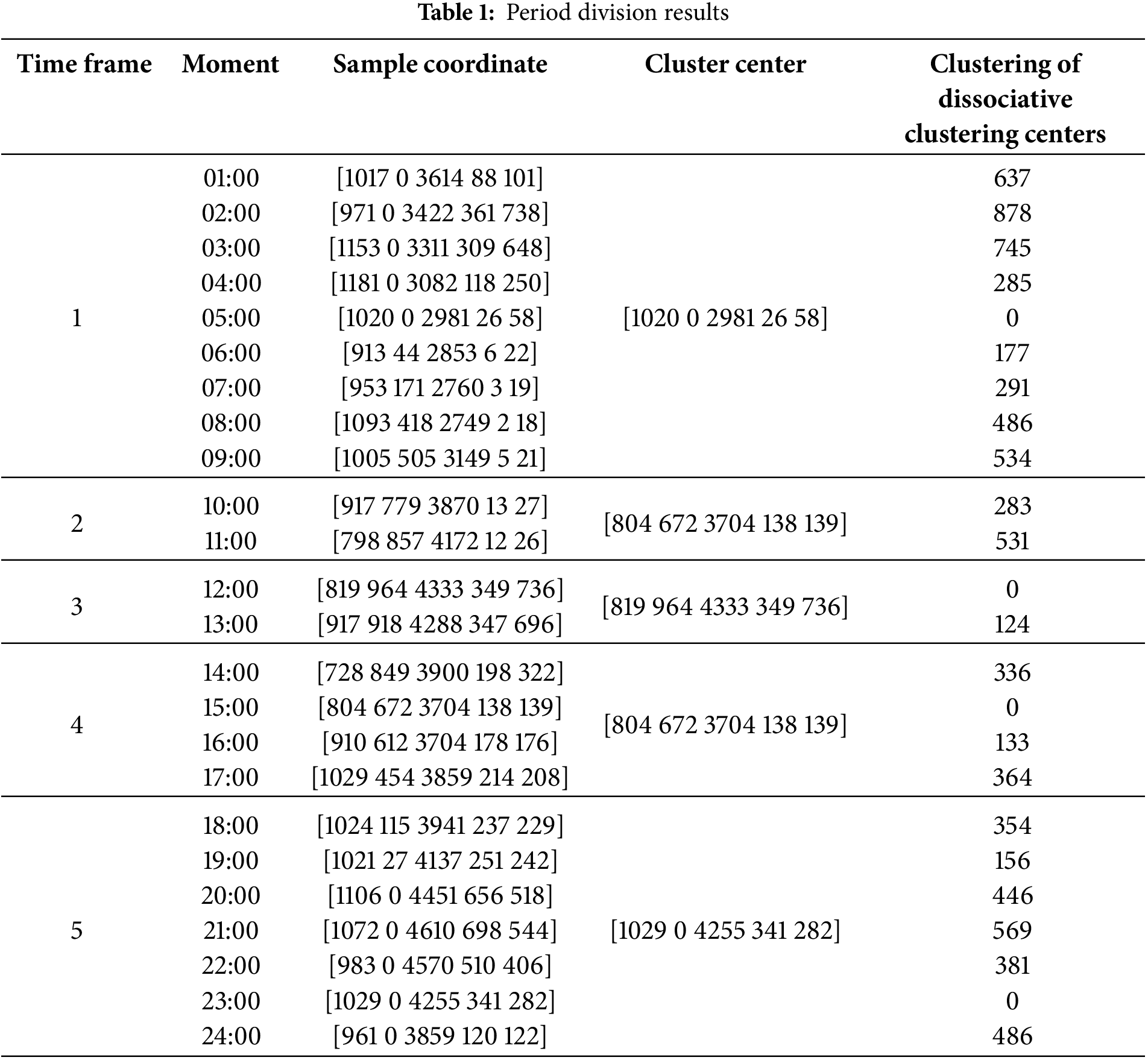
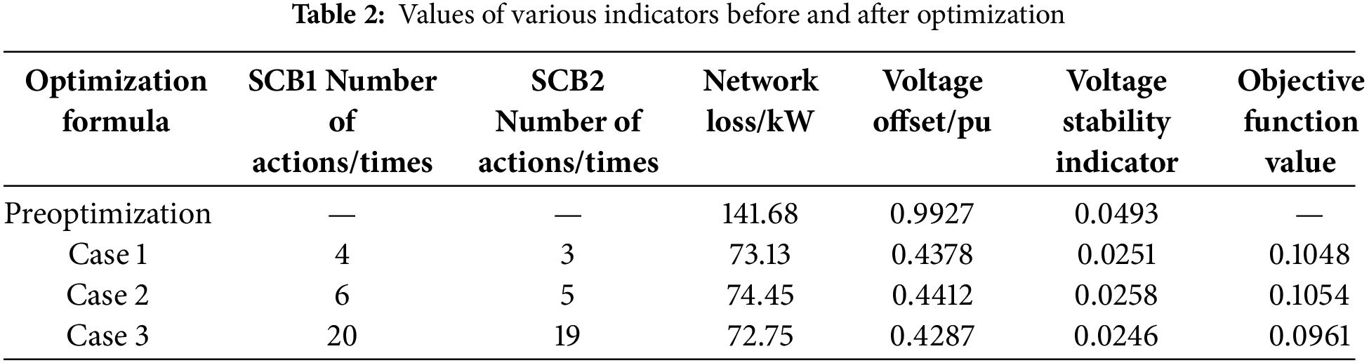
Then, the time division results of Table 1 are dynamically optimized, and the optimization results are recorded as Case 1. In order to verify the effectiveness of the spatio-temporal decoupling strategy proposed in this paper, three cases are set up for comparative experiments. Case 1 is the space-time decoupling strategy of dynamic reactive power optimization proposed in this paper. Case 2 is the space-time decoupling strategy proposed in Reference [7]. Case 3 is the static reactive power optimization strategy without considering the constraint of the number of capacitor bank actions, the results of the capacitor bank input are shown in Figs. 9 and 10, and the 24-h average comparison results of each index are shown in Table 2.

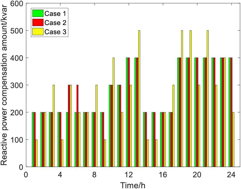
Figure 9: SCB1 reactive power compensation comparison diagram

Figure 10: SCB2 reactive power compensation comparison diagram

From Figs. 9 and 10, it can be seen that in Case 1, SCB1 performed 4 cuts at 10, 12, 14, and 18 h, respectively, and SCB2 performed 3 cuts at 10, 14, and 18 h, respectively, to meet the action number constraints. In case 2, SCB1 performed 6 cuts at 5, 7, 10, 12, 14 and 18 h, respectively, and SCB2 performed 5 cuts at 3, 5, 10, 14 and 18 h, respectively. Compared with Case 2, Case 1 has a 50% reduction in SCB1 and a 66.67% reduction in SCB2 in the number of capacitor bank switching times. The main reason for the difference in the number of actions is that the fluctuation of load and new energy power is the main reason for the different operating states of each hour section of the distribution network. The space-time decoupling strategy proposed in Case 1 starts from the difference between load and new energy power fluctuations, and then performs clustering division, so the time period division is more reasonable. Although the number of actions in Reference [7] is limited to the allowable range, it is divided from the final optimization results, ignoring the essential reasons that lead to different operating states in each period, and the division results have certain compromise. The number of actions of SCB1 and SCB2 in case 3 is 20 and 19, respectively, which is greatly increased compared with Case 1 and Case 2. The main reason is that Case 3 does not consider the constraint of the number of actions of the capacitor bank.

It can be seen from Table 2 that the network loss, voltage offset and voltage stability indexes of Case 2 are reduced by 48.16%, 55.56% and 48.28% respectively compared with those before optimization. Compared with Case 2, Case 1 continues to reduce 0.93% in network loss, 0.34% in voltage offset and 0.62% in voltage stability index. The network loss, voltage offset and voltage stability indexes of Case 3 are reduced by 48.65%, 56.81% and 50.10% respectively compared with those before optimization.

Based on the above analysis, the three indicators of Case 1 and Case 3 are not much different, but the number of actions of the capacitor bank in Case 1 is greatly reduced, and compared with Case 2, the indicators of Case 1 are improved, which effectively illustrates the effectiveness of the space-time decoupling strategy proposed in this paper.

5.3 Algorithm Analysis in this Paper

In order to verify the advantages of the cross-feedback hybrid optimization algorithm in this paper, three cases are set up. Cases 1–3 are the combination of TAMAHA algorithm, AHA algorithm and PSO algorithm and GA algorithm, respectively. The objective function values of each hour segment before and after optimization are shown in Fig. 11. As can be seen from the figure, the reactive power optimization effect of the optimization strategy proposed in Case 1 is better than that of other cases in all hours of the day.

Figure 11: Full day optimization satisfaction

Table 3 shows the reactive power optimization results in different cases, in which each index is the average value of 24 h. It can be seen from Table 3 that: 1) On the basis of ensuring the quality of electrical voltage, Case 1, Case 2 and Case 3 can respectively reduce the active power network loss by 48.4%, 48.0% and 47.7%, and Case 1 is better in reducing the active power network loss. 2) Case 1, Case 2 and Case 3 reduce the voltage deviation by 55.9%, 55.2% and 54.8%, respectively, and Case 1 can better reduce the voltage deviation. 3) Case 1, Case 2 and Case 3 reduce the voltage stability index by 49.1%, 48.5% and 47.5%, respectively, and Case 1 is more beneficial to optimize the system stability. 4) The advantages of Case 1 in reducing voltage deviation, reducing active power network loss and improving system stability make the comprehensive optimization results of each hour segment optimal.

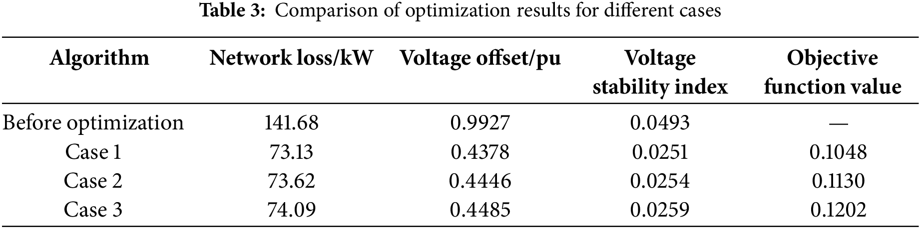
Fig. 12 shows the results of node voltage comparison after optimization in the 23rd hour segment. As can be seen from Fig. 12, system voltage levels were optimized in different degrees in all three cases. The voltage of all nodes after optimization can meet the power quality requirements, and the voltage quality after optimization in Case 1 is even better.

Figure 12: Comparison of optimized node voltages

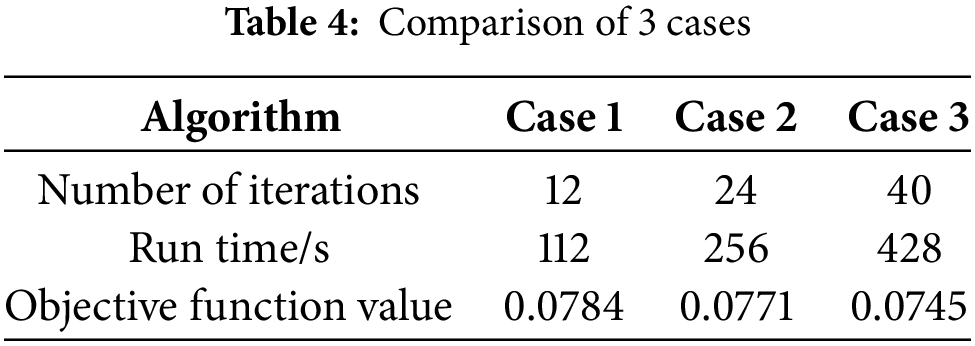
Fig. 13 and Table 4 show the comparison of convergence curves and optimization speeds in the 11th hour segment of the three cases. Fig. 8 shows that the PSO algorithm is prone to fall into local optimality in the late iteration period, mainly due to the low population diversity in the late iteration period. Due to the existence of the access table, the AHA algorithm mainly updates the position of the individual according to the optimal individual in the early optimization, and tracks the position of other individuals according to the length of the visit time in the later period, so as to improve its global optimization ability. Due to the addition of the adaptive mutation operator based on population aggregation degree, the TAMAHA algorithm can maintain excellent population diversity in the late iteration, and has strong global search ability, which reduces the possibility of falling into the local optimal. It can be seen from Table 4 that Case 1 has obvious advantages in terms of iteration times and optimization time compared with other cases, and the value of objective function is low. Therefore, the cross-feedback hybrid algorithm represented by Case 1 has better optimization effect and faster optimization speed.

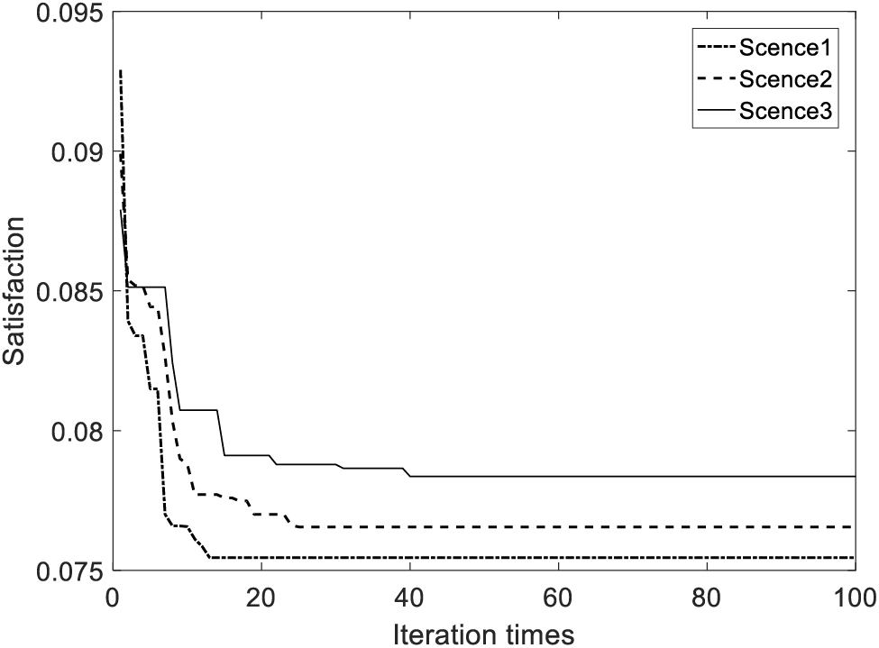
Figure 13: Convergence curve

6  Conclusion

The main conclusions of this paper are:

1) Considering the uncertainty of the source load power, this paper establishes a dynamic reactive power optimization model with the minimum active power loss and voltage fluctuation of the distribution network and the optimal voltage stability margin. Simulation results show that the model proposed in this paper can improve the voltage level, improve the system operation stability, and further reduce the active power loss. Therefore, the model proposed in this paper is more suitable for the actual needs.

2) A clustering-local relaxation-correction reactive power optimization decoupling strategy is proposed, which comprehensively considers the influence of new energy output, EV charging load, and residential power load fluctuations, uses the k-medoids clustering algorithm to divide the time period, and then performs static reactive power optimization for each time period. Therefore, the original problem is decoupled to a static reactive power optimization problem, which reduces the difficulty of solving. High reactive power optimization effect can be obtained while CB operation times constraint is satisfied.

3) According to the characteristics of decision variables, the cross-feedback hybrid algorithm formed by the combination of the improved artificial hummingbird algorithm and the genetic algorithm is used to solve the model. The results show that the proposed algorithm has fast optimization speed and strong global search ability and can effectively solve non-convex and nonlinear reactive power optimization problems of mixed integers.

The research focus of this paper is on the space-time decoupling method and the solution algorithm of the model, and the uncertainty processing method is more traditional. Therefore, in future research, more effective uncertainty processing methods need to be further studied.

Acknowledgement: Not applicable.

Funding Statement: This research was funded by the “Research and Application Project of Collaborative Optimization Control Technology for Distribution Station Area for High Proportion Distributed PV Consumption (4000-202318079A-1-1-ZN)” of the Headquarters of the State Grid Corporation.

Author Contributions: The authors contributed significantly to this research paper by: Conceptualizing the problem and designing the methodology, Collecting and processing data on load, wind, PV, and EV charging: Chenxu Wang; Developing and implementing the improved artificial hummingbird algorithm and cross-feedback hybrid optimization algorithm; Analyzing results and drawing conclusions: Rui Yuan; Writing and editing the paper: Jing Bian. All authors reviewed the results and approved the final version of the manuscript.

Availability of Data and Materials: The authors confirm that the data used in this study are available on request.

Ethics Approval: Not applicable.

Conflicts of Interest: The authors declare no conflicts of interest to report regarding the present study.

References

1. Li P, Sheng W, Duan Q, Li Z, Zhu C, Zhang X. A lyapunov optimization-based energy management strategy for energy hub with energy router. IEEE Trans Smart Grid. 2020 Nov;11(6):4860–70. doi:10.1109/TSG.2020.2968747. [Google Scholar] [CrossRef]

2. Hu S, Xiang Y, Liu J, Gu C, Zhang X, Tian Y, et al. Agent-based coordinated operation strategy for active distribution network with distributed energy resources. IEEE Trans Ind Appl. 2019 Jul–Aug;55(4):3310–20. doi:10.1109/TIA.2019.2902110. [Google Scholar] [CrossRef]

3. Zhu J, Mo X, Xia Y, Guo Y, Chen J, Liu M. Fully-decentralized optimal power flow of multi-area power systems based on parallel dual dynamic programming. IEEE Trans Power Syst. 2022 Mar;37(2):927–41. doi:10.1109/TPWRS.2021.3098812. [Google Scholar] [CrossRef]

4. Kuang H, Mu XX, Sheng Qin R. Dynamic reactive power optimization model for a wind farms and energy storage combined system. 2020 IEEE 20th International Conference on Communication Technology (ICCT); Nanning, China; 2020. p. 1625–9. doi:10.1109/ICCT50939.2020.9295876 [Google Scholar] [CrossRef]

5. Vijayan V, Mohapatra A, Singh SN, Dewangan CL. An efficient modular optimization scheme for unbalanced active distribution networks with uncertain EV and PV penetrations. IEEE Trans Smart Grid. 2023 Sep;14(5):3876–88. doi:10.1109/TSG.2023.3234551. [Google Scholar] [CrossRef]

6. Kamel S, Ramadan A, Ebeed M, Yu J, Xie K, Wu T. Assessment integration of wind-based DG and DSTATCOM in Egyptian distribution grid considering load demand uncertainty. In: 2019 IEEE Innovative Smart Grid Technologies—Asia (ISGT Asia). Chengdu, China; 2019. p. 1288–93. doi:10.1109/ISGT-Asia.2019.8881437. [Google Scholar] [CrossRef]

7. Luo P, Sun JH. Research on dynamic reactive power optimization decoupling method of active distribution network. High Volt Technol. 2021;4:1323–33. doi:10.13336/j.1003-6520.hve.2020005. [Google Scholar] [CrossRef]

8. Chen L, Deng Z, Xu X. Two-stage dynamic reactive power dispatch strategy in distribution network considering the reactive power regulation of distributed generations. IEEE Trans Power Syst. 2019 Mar;34(2):1021–32. doi:10.1109/TPWRS.2018.2875032. [Google Scholar] [CrossRef]

9. Rather ZH, Chen Z, Thøgersen P, Lund P. Dynamic reactive power compensation of large-scale wind integrated power system. IEEE Trans Power Syst. 2015 Sep;30(5):2516–26. doi:10.1109/TPWRS.2014.2365632. [Google Scholar] [CrossRef]

10. Deng Z, Liu M, Ouyang Y, Lin S, Xie M. Multi-objective mixed-integer dynamic optimization method applied to optimal allocation of dynamic var sources of power systems. IEEE Trans Power Syst. 2018 Mar;33(2):1683–97. doi:10.1109/TPWRS.2017.2724058. [Google Scholar] [CrossRef]

11. Chi Y, Xu Y, Zhang R. Many-objective robust optimization for dynamic VAR planning to enhance voltage stability of a wind-energy power system. IEEE Trans Power Deliv. 2021 Feb;36(1):30–42. doi:10.1109/TPWRD.2020.2982471. [Google Scholar] [CrossRef]

12. Ding T, Liu S, Yuan W, Bie Z, Zeng B. A two-stage robust reactive power optimization considering uncertain wind power integration in active distribution networks. IEEE Trans Sustain Energy. 2016 Jan;7(1):301–11. doi:10.1109/TSTE.2015.2494587. [Google Scholar] [CrossRef]

13. Liang GK, Fang J, Wang ZJ, Qin Y, Cui YP, Yin K, et al. A dynamic optimization model for energy conservation and loss reduction in urban distribution networks with load voltage, capacity, and distribution transformers. Power Automation Equipment. 2019;39(12):114–20. doi:10.16081/j.epae.201911019. [Google Scholar] [CrossRef]

14. Geng G, Liang J, Harley RG, Qu R. Load profile partitioning and dynamic reactive power optimization. In:2010 International Conference on Power System Technology; Zhejiang, China; 2010. p. 1–8. doi:10.1109/POWERCON.2010.5666514. [Google Scholar] [CrossRef]

15. Xiao J, Liu TQ, Su P. Reactive power optimization for time-sharing power systems based on dual population particle swarm optimization. Power Grid Technol. 2009;33:72–7. [Google Scholar]

16. Shadman Abid M, Apon HJ, Morshed KA, Ahmed A. Optimal planning of multiple renewable energy-integrated distribution system with uncertainties using artificial hummingbird algorithm. IEEE Access. 2022;10:40716–30. doi:10.1109/ACCESS.2022.3167395. [Google Scholar] [CrossRef]

17. Ismail B, Wahab NIA, Othman ML, Radzi MAM, Vijayakumar KN, Rahmat MK, et al. New line voltage stability index (BVSI) for voltage stability assessment in power system: the comparative studies. IEEE Access. 2022;10:103906–31. doi:10.1109/ACCESS.2022.3204792. [Google Scholar] [CrossRef]

18. Ren Z, Xu Z, Wang H. The strategy selection problem on artificial intelligence with an integrated VIKOR and AHP method under probabilistic dual hesitant fuzzy information. IEEE Access. 2019;7:103979–99. doi:10.1109/ACCESS.2019.2931405. [Google Scholar] [CrossRef]

19. Yang D, Cheng H, Ma Z, Yao L, Zhu Z. Dynamic VAR planning methodology to enhance transient voltage stability for failure recovery. J Mod Power Syst Clean Energy. 2018 Jul;6(4):712–21. doi:10.1007/s40565-017-0353-5. [Google Scholar] [CrossRef]

20. Li JC, Li L. A hybrid genetic algorithm based on information entropy and game theory. IEEE Access. 2020;8:36602–11. doi:10.1109/ACCESS.2020.2971060. [Google Scholar] [CrossRef]

21. Mohammad F, Kang, DK, Ahmed MA, Kim YC. Energy demand load forecasting for electric vehicle charging stations network based on ConvLSTM and BiConvLSTM architectures. IEEE Access. 2023;11:67350–69. doi:10.1109/ACCESS.2023.3274657. [Google Scholar] [CrossRef]