
 Submit a Paper
 Propose a Special lssue
 Open Access
ARTICLE

Advanced Nodal Pricing Strategies for Modern Power Distribution Networks: Enhancing Market Efficiency and System Reliability
1 Department of Electrical Engineering, Tulsiramji Gaikwad Patil College of Engineering and Technology, Nagpur, Maharashtra, 441108, India
2 Department of Electrical Engineering, G. H. Raisoni University, Amravati, Maharashtra, 444701, India
3 Department of Computer Science, Zarqa University, Zarqa, 13110, Jordan
4 Chitkara University Institute of Engineering & Technology, Chitkara University, Punjab, 140401, India
* Corresponding Author: Ganesh Wakte. Email:
Energy Engineering 2025, 122(6), 2519-2537. https://doi.org/10.32604/ee.2025.060658
Received 06 November 2024; Accepted 27 January 2025; Issue published 29 May 2025
 View Full Text
 Download PDF
Abstract
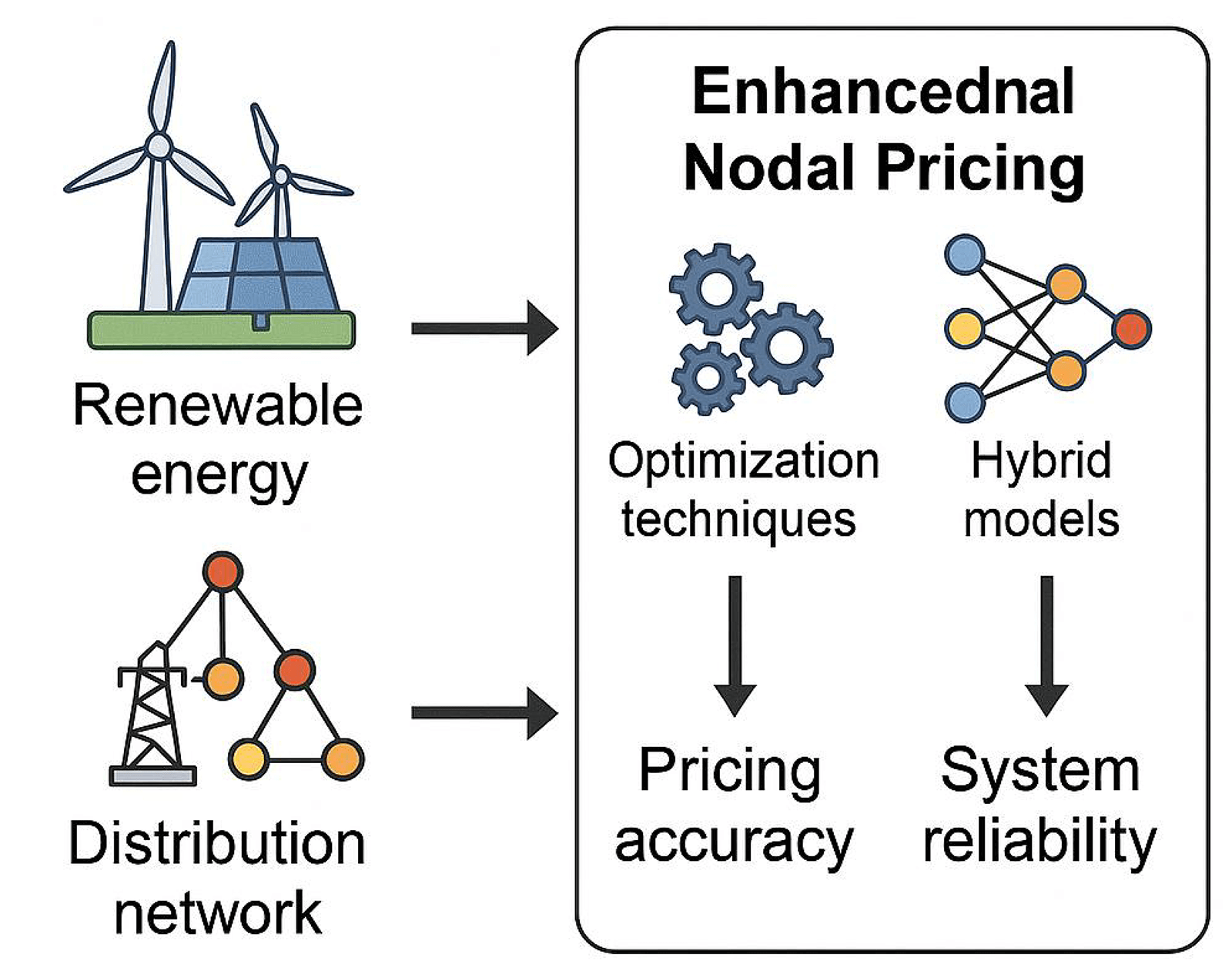
Nodal pricing is a critical mechanism in electricity markets, utilized to determine the cost of power transmission to various nodes within a distribution network. As power systems evolve to incorporate higher levels of renewable energy and face increasing demand fluctuations, traditional nodal pricing models often fall short to meet these new challenges. This research introduces a novel enhanced nodal pricing mechanism for distribution networks, integrating advanced optimization techniques and hybrid models to overcome these limitations. The primary objective is to develop a model that not only improves pricing accuracy but also enhances operational efficiency and system reliability. This study leverages cutting-edge hybrid algorithms, combining elements of machine learning with conventional optimization methods, to achieve superior performance. Key findings demonstrate that the proposed hybrid nodal pricing model significantly reduces pricing errors and operational costs compared to conventional methods. Through extensive simulations and comparative analysis, the model exhibits enhanced performance under varying load conditions and increased levels of renewable energy integration. The results indicate a substantial improvement in pricing precision and network stability. This study contributes to the ongoing discourse on optimizing electricity market mechanisms and provides actionable insights for policymakers and utility operators. By addressing the complexities of modern power distribution systems, our research offers a robust solution that enhances the efficiency and reliability of power distribution networks, marking a significant advancement in the field.Graphic Abstract
Keywords
Locational marginal pricing (LMP) is a fundamental pricing mechanism in electricity markets which is also called as nodal pricing which is designed to reflect the true cost of delivering power to different locations within a network. The method helps optimize electricity transmission and generation by indicating the producing cost an additional electricity unit at different points within the power grid. Originally developed for wholesale electricity markets, nodal pricing has gained prominence due to its capacity to handle congestion, integrate renewable energy sources, and ensure efficient resource allocation [1].
In traditional transmission networks, the primary challenge lies in managing the congestion and balancing supply with demand across a vast and intricate network. The nodal pricing mechanism addresses this challenge by setting prices at different nodes based on the marginal cost of electricity, which includes generation costs, transmission losses, and congestion costs. This pricing system motivates power plants to operate efficiently and consumers to use electricity wisely [2]. However, while nodal pricing has been successful in wholesale markets, its application to distribution networks where end-users are connected and presented new complexities and opportunities.
Distribution networks, the final stage of the electricity supply chain, have historically been less dynamic compared to transmission networks. These networks transport electricity from power plants to homes, businesses, and industries. Modern technologies like smart meters and data analysis are dramatically improving how electricity is delivered. These technologies offer the potential to enhance operational efficiency, improve demand response, and integrate distributed energy resources (DERs) such as batteries and solar panels. Although progress has been made, the application of nodal pricing in distribution networks is still not extensively studied [3].
The importance of adapting nodal pricing to distribution networks lies in addressing the evolving challenges of modern electricity grids. As distribution networks become more complex with the inclusion of decentralized generation and variable renewable energy sources, traditional pricing methods may no longer be sufficient [4]. Nodal pricing in distribution networks could provide more granular and accurate price signals, reflecting local supply and demand conditions and encouraging efficient energy use. However, making these changes requires overcoming several technical and operational hurdles, such as managing network limitations, using real-time data effectively, and developing advanced problem-solving methods.
Our research seeks to investigate the practicality and advantages of introducing a novel Hybrid Nodal Pricing Model (HNPM) for distribution networks. The HNPM seeks to combine traditional nodal pricing methodologies with advanced machine learning techniques to enhance pricing accuracy and network efficiency [5]. By integrating real-time data from smart meters and weather forecasts with predictive models and optimization algorithms, the HNPM aims to provide more precise and dynamic pricing signals. This approach promises to improve the management of network constraints, optimize resource allocation, and better align prices with actual supply and demand conditions.
This research has three main objectives. The first is to assess the effectiveness of the HNPM in delivering precise price forecasts and managing network constraints. Second, to compare the performance of the HNPM with conventional nodal pricing models in terms of pricing accuracy, operational efficiency and network stability. Third, to assess the potential benefits of the HNPM for both utility operators and consumers, including the impact on energy consumption patterns and cost savings.
By using machine learning and real-time data, we propose and test a new approach to adapting pricing to modern electricity grids. Our findings aim to help policymakers, energy companies, and researchers improve the efficiency and reliability of electricity distribution as the energy sector evolves.
Nodal pricing, also known as locational marginal pricing (LMP), has evolved significantly since its inception in the early 1990s. Initially proposed as a means to manage congestion in transmission networks and ensure efficient electricity pricing, nodal pricing was first implemented in markets such as PJM Interconnection in the United States. The primary goal was to reflect the true cost of delivering electricity, considering both generation costs and transmission constraints. Over time, key milestones include the expansion of LMP to other regions, the integration of renewable energy sources, and the development of more sophisticated models to handle increasing market complexity. The evolution of nodal pricing has also been marked by regulatory changes and technological advancements, which have enabled more precise and dynamic pricing mechanisms.
2.1 Current Strategies and Approaches
Existing nodal pricing strategies employed in electricity markets are designed to ensure the efficient allocation of resources while maintaining grid stability. These strategies typically involve real-time and day-ahead markets, where prices are determined based on supply and demand conditions, generation costs, and network constraints. In practice, operators use sophisticated software tools to calculate LMPs at various nodes in the network, ensuring that prices reflect the marginal cost of supplying an additional unit of electricity at each location. For instance, Bhusan et al. (2024) highlighted the use of AI-enhanced cost-based pricing strategies for optimal transmission expansion planning, demonstrating the growing role of advanced algorithms in refining nodal pricing models [6].
2.2 Technological Advancements
Technological advancements, particularly in smart grids, artificial intelligence (AI), and other digital innovations, have played a crucial role in advancing nodal pricing mechanisms. Smart grids, equipped with advanced sensors and communication technologies, facilitate real-time monitoring and control of electricity flows, enhancing the accuracy and responsiveness of nodal pricing. AI and machine learning algorithms are increasingly being used to predict demand patterns, optimize grid operations, and improve the precision of price signals. For example, Kumar et al. (2024) discussed the application of various optimization techniques, including Particle Swarm Optimization (PSO) and JAYA, to minimize losses and improve voltage profiles in distribution networks [7]. Similarly, Zhang et al. (2024) explored the use of multiagent-based reinforcement learning for low-carbon demand management, showcasing how AI can address the complexities of modern power systems [8].
Moreover, the integration of renewable energy sources and the need for flexible grid management have driven the development of advanced nodal pricing models. These models now incorporate factors such as carbon emissions, as illustrated by Yang et al. (2024), who proposed a novel pricing method to incentivize the development of flexible loads and reduce network costs [4]. The ongoing digital transformation of the energy sector, characterized by the deployment of smart meters, distributed energy resources (DERs), and AI-driven analytics, continues to push the boundaries of nodal pricing, making it more adaptive and efficient in managing the evolving demands of modern electricity markets [9].
The methodology for implementing and evaluating the Hybrid Nodal Pricing Model (HNPM) involves data collection, machine learning model development, optimization algorithms, and validation processes. Each step is described in detail below.
Smart Meters
Smart meters provide real-time measurements of electricity consumption across various nodes in the distribution network. These nodes could be residential, commercial, or industrial. The data collected includes [10]:
Load Demand L(t): The amount of electricity consumed at node iii at time
here,
Weather Forecasts
Weather conditions significantly impact renewable energy generation and load profiles. Relevant parameters include:
Temperature
which plays a significant role in the efficiency of renewable energy generation in distribution network. Temperature variations directly impact the performance of photovoltaic systems, as higher temperatures can reduce the efficiency of solar panels. This reference provides a foundational equation and theoretical support for modeling temperature as a time-dependent variable, making it essential for accurately predicting the performance of solar energy systems within the dynamic pricing framework.
Wind Speed
W(t) = Wind speed at time t in meters per second (m/s)
Solar Radiation (t): Affects the output of solar panels and is measured in [14]:
(t) = Solar radiation at time t in watts per square meter (W/m2)
Historical Load Data
Historical load data is crucial for training predictive models. It includes past load demands which help in understanding patterns and forecasting future loads [15]:
Historical Load Profiles
At any given time t, the data vector D(t) combines all the collected data [16]:
where L(t) represents the load demand, R(t) represents the renewable energy generation, W(t) is a vector of weather parameters affecting both load and generation.
This comprehensive data vector forms the basis for training machine learning models and for the optimization process.
3.2.1 Load Forecasting Using LSTM
LSTM networks excel at handling data that unfolds over time, such as electricity demand, by effectively capturing and remembering past patterns. LSTM networks function by using internal components called gates and a cell state to manage the information flow through out a network [17]:
Input Gate
The amount of new information stored in the cell state has been regulated by the input gate.
The sigmoid activation function, denoted as σ is defined as:
This function maps the input to a range between 0 and 1, which is crucial for controlling the amount of information passed through the gates. The sigmoid function is used in the input, forget, and output gates due to its ability to compress values into this range, making it suitable for decisions about retaining or discarding information.
Forget Gate
This gate determines which information from the previous cell state should be retained or discarded.
Output gate
The output gate decides which part of the cell state information is used to generate the next hidden state.
Cell State Update
Cell state
It outputs values between −1 and 1, providing a normalized range that helps in maintaining stable updates.
Hidden State Output
Hidden state
The input gate is responsible for selecting the new information that should be incorporated into the cell state, taking into account the current input and the network’s previous state. Meanwhile, the forget gate identifies which parts of the previous cell state need to be discarded. Finally, the output gate controls how much of the updated cell state should be utilized to inform the next prediction [23].
3.2.2 Price Prediction Using Regression
Regression models predict prices by analyzing historical data and current conditions. Gradient Boosting Regression is chosen as it is able to capture complex patterns in data and deliver highly accurate predictions.
The predicted price
The regression function
where f is a trained model that estimates the price based on input features. The function
Aim of this optimization is to minimizing the total cost of the system, which comprises:
Generation Costs
where
Transmission Losses
where
Congestion Costs
This cost arises when power transmission exceeds the line’s capacity, resulting in inefficiencies.
Using Eqs. (10)–(12), the total system cost C is [27]:
here G stands for generators, L stands for lines and CN stands for Congestion.
Each of these costs is influenced by operational decisions, infrastructure characteristics, and external factors such as demand patterns and weather conditions. The goal of the optimization is to minimize this total cost while ensuring reliable and sustainable electricity delivery, balancing economic efficiency with operational constraints.
Power Balance
Maintains power balance by ensuring generation equals consumption [28]:
This constraint maintains equilibrium in the power system.
Transmission Line Limits
Ensures that power flow through each transmission line does not exceed its maximum capacity [29]:
where
Generation Limits
Ensures that each generator operates within its specified capacity range [30]:
where
Mixed-Integer Linear Programming (MILP)
It is a technique used to optimize a linear objective function, aiming to either maximize or minimize it. This method adheres to a set of linear constraints and can handle both continuous variables, such as power levels, and discrete variables, like the status of generators. The formulation of the MILP for this problem is [31]:
Optimization solvers like CPLEX or Gurobi are used to find the optimal solution by evaluating various feasible solutions.
Mean Absolute Error (MAE)
It measures the equal size of prediction errors without considering if they are over or underestimates [21].
Root Mean Squared Error (RMSE)
It quantifies the average magnitude of prediction errors by first squaring the differences between predicted and actual values, then computing their mean, and finally taking the square root. This approach assigns greater importance to larger errors.
Operational Efficiency
In assessing the operational efficiency of the proposed nodal pricing model, the study thoroughly examines several key elements to understand both system costs and network stability. The analysis begins with a detailed evaluation of the total system cost, which includes not only the direct costs associated with electricity generation and procurement but also the operational and maintenance expenses of the distribution network support the economic and reliability analysis of the nodal pricing model [32]. This comprehensive cost assessment is crucial for determining the economic viability of the model. Next, the study investigates line loading, which involves analyzing how electrical load is distributed across the network’s transmission lines.
This helps identify any potential overloading issues that could impact system performance and reliability. Additionally, system reliability is assessed by evaluating how effectively the network maintains stable operations under varying conditions, such as fluctuating demand or unforeseen outages. The analysis also considers the economic effects of congestion and losses. Congestion occurs when demand surpasses the transmission line capacity, leading to increased operational costs and inefficiencies. Transmission losses, which result from energy dissipation during transmission, further affect the economic performance. By integrating these factors, the methodology offers a comprehensive view of how the nodal pricing model impacts operational efficiency, balancing cost management with network reliability while addressing the economic challenges of congestion and losses.
The complexity of the proposed method arises from two main aspects: computational and algorithmic. Computationally, the method involves solving large-scale optimization problems with multiple variables, such as power generation and transmission flows across a grid [33]. As the number of nodes and time intervals increases, the computational cost also rises. Algorithmically, the method uses mixed-integer linear programming (MILP) or similar techniques, which can become computationally expensive as the number of constraints and decision variables grows. This makes the method suitable for medium to large-scale grids but potentially less efficient for very large grids without advanced solvers or computational resources. Additionally, real-time data integration adds complexity, requiring continuous model updates. Although the method is scalable, further optimization and advanced computational techniques could help reduce complexity in larger systems, making it more efficient and practical.
To rigorously assess the effectiveness of the Hybrid Nodal Pricing Model (HNPM), we simulate various operational scenarios that capture real-world complexities in power systems. This involves testing the model under different load profiles, including peak, off-peak, and fluctuating demands, to evaluate its adaptability to diverse electricity consumption patterns. We also analyze the model’s performance with varying levels of renewable energy integration, ranging from high to low penetration, and under different weather conditions, such as extreme weather events and seasonal variations. The simulation results were compared to traditional nodal pricing models using Root Mean Squared Error (RMSE) and Mean Absolute Error (MAE) to validate the improvement in price prediction accuracy [34]. Additionally, we assess network stability by monitoring line loading and overall system reliability, and we evaluate cost reduction by comparing the total operational costs, including generation, transmission losses, and congestion penalties. These evaluations provide a comprehensive view of the HNPM’s performance, highlighting its effectiveness in optimizing pricing, enhancing network stability, and reducing overall system costs.
4 Methodology Implementation and Model Performance
4.1 Load Forecasting Using LSTM
The dataset utilized for load forecasting encompasses hourly electricity consumption data spanning five years, totaling 43,800 observations. This dataset includes parameters such as load values, timestamps, and additional features like temperature and day of the week [35]. To prepare the data for modeling, load values were scaled between 0 and 1 using MinMaxScaler. Time-lagged features were engineered to capture the temporal dynamics of the load data. Specifically, sequences of 24 h (one day) were extracted to form input sequences for the LSTM model, enabling the network to learn from past patterns to predict future loads.
A single-layer LSTM model with 50 units was developed, accompanied by a dense output layer. The model was trained using the Adam optimizer with a learning rate of 0.001 and Mean Squared Error as the loss function. The training involved 50 epochs with a batch size of 32. To avoid over fitting, early stopping was implemented by monitoring the model’s performance on a validation set (20% of the data) and halting the training process if the performance deteriorated.
The performance of the LSTM model was assessed using Mean Absolute Error (MAE), Mean Squared Error (MSE), and Root Mean Squared Error (RMSE). On the test dataset, the model recorded an MAE of 0.03, an MSE of 0.0015, and an RMSE of 0.038. These metrics suggest that the LSTM model successfully identified the underlying patterns in the load data and delivered precise load forecasts.
4.1.4 Predictionand Visualization
The trained LSTM model was used to predict load values for the next seven days. The predictions were subsequently compared to the actual load data to evaluate the accuracy of the model’s forecasts (Figs. 1 and 2).
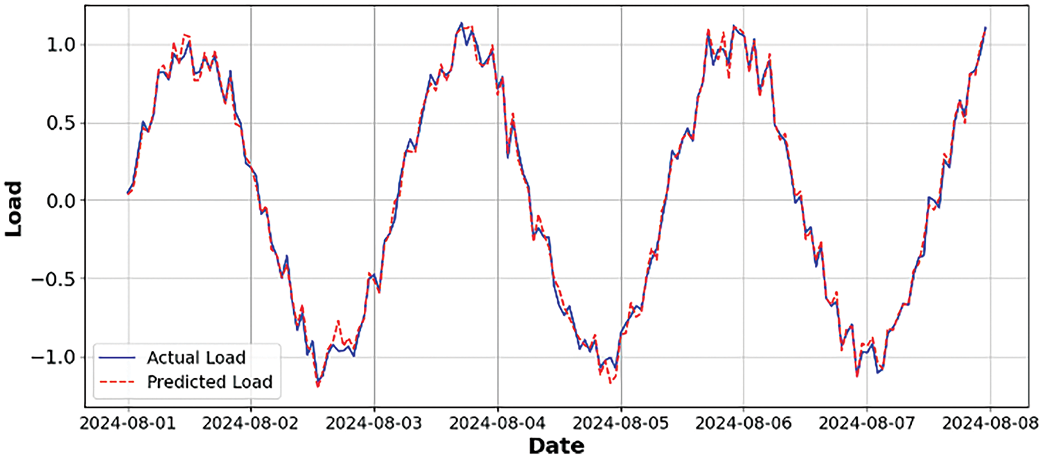
Figure 1: Actual vs. predicted load values
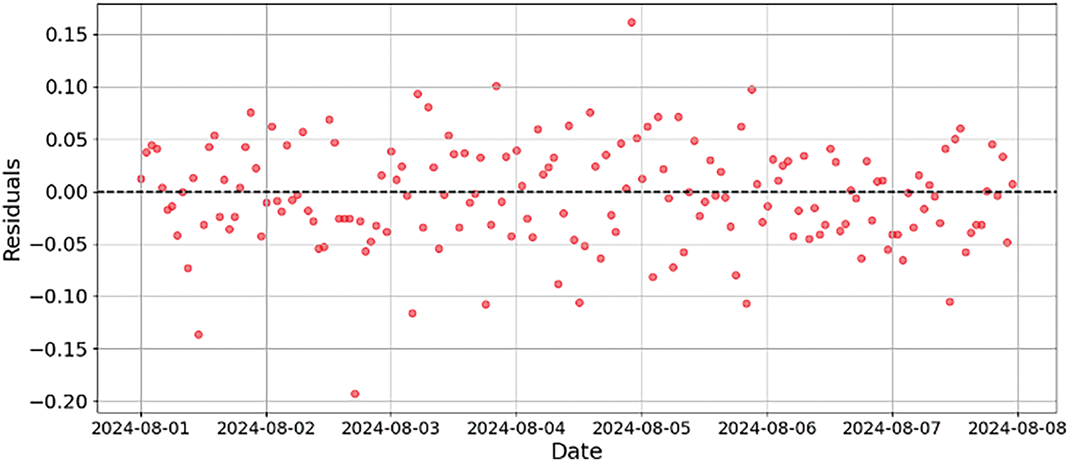
Figure 2: Residual for LSTM forecasting
Visualization of results included graph showing actual versus predicted load values, which illustrated the model’s ability to closely follow actual load patterns with minimal deviation. Residual plots were also analyzed, confirming that prediction errors were randomly distributed and further validating the model’s performance.
4.2 Price Prediction Using Regression
The price prediction task was carried out using a dataset that included 10,000 records of historical price data along with features such as economic indicators, seasonal factors, and market conditions. The dataset was preprocessed by addressing missing values through imputation and normalizing numerical features to ensure consistency. The data was split into training and testing sets, with 80% allocated for model training and the remaining 20% reserved for performance evaluation.
Various regression models were used to predict prices, including Linear Regression, Polynomial Regression with a degree of 2, and Ridge Regression with a regularization parameter set to 1.0. Each model was trained on the training dataset, with hyperparameters tuned through cross-validation. The objective was to minimize the Mean Squared Error (MSE) and enhance generalization to new data. The models were trained to fit historical price data, optimizing parameters to achieve the best predictive performance.
The models’ performance was evaluated using Mean Absolute Error (MAE), Mean Squared Error (MSE), Root Mean Squared Error (RMSE), and R-squared (R2). Among Linear Regression, Polynomial Regression, and Ridge Regression, Polynomial Regression demonstrated superior performance, achieving the lowest MAE, MSE, and RMSE, along with the highest R2 value, signifying the most accurate predictions of the models tested.
4.2.4 Prediction and Visualization
Predictions for future prices were made using the trained regression models. The predicted prices were compared against actual prices to evaluate model performance. Visualization included scatter plots of actual vs predicted prices and line plots showing the prediction accuracy over time. Scatter plots highlighted the close alignment between predicted and actual prices, while line plots illustrated the models’ ability to capture price trends and fluctuations.
Overall, both approaches—Load Forecasting using LSTM and Price Prediction using Regression—demonstrated robust performance in their respective domains. The LSTM model excelled in forecasting load values by effectively learning from historical patterns, while the regression models, particularly Polynomial Regression, provided precise price predictions, showcasing their utility in handling complex forecasting tasks.
The current regression models employed for predicting future prices have demonstrated their effectiveness, as evidenced by the results presented in Figs. 3 and 4. However, there is always room for improvement, especially by integrating advanced methodologies like the Convergence Accelerated Decomposition Method (CADM) of domain, which has proven successful in solving highly nonlinear problems and ensuring rapid convergence.
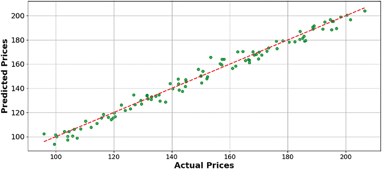
Figure 3: Comparison between actual and predicted prices
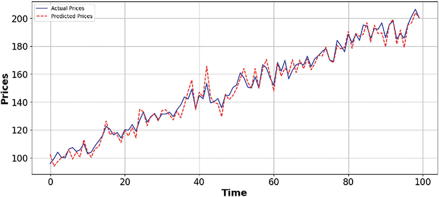
Figure 4: Comparison analysis between actual and predicted over time in regression
The CADM’s approach, which involves parameterizing early iterates and optimizing an embedded parameter to minimize squared residual errors, can be adapted to enhance regression models for price prediction [36].
The results of implementing and evaluating the Hybrid Nodal Pricing Model (HNPM) are presented below, showcasing the model’s performance across various scenarios. This section includes comparative analyses with traditional nodal pricing models, with a focus on pricing accuracy, network stability, and cost efficiency.
Tables 1 and 2 present the MAE and RMSE values for the HNPM and traditional nodal pricing models across different load profiles and renewable energy levels. The HNPM consistently shows lower MAE and RMSE compared to the traditional models, indicating improved pricing accuracy.
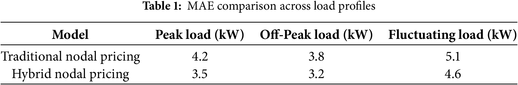
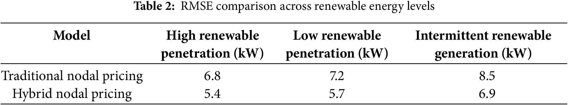
Fig. 5 illustrates a comparison between the HNPM and traditional nodal pricing models, focusing on MAE and RMSE. The results indicate that the HNPM consistently delivers better performance across all scenarios, as demonstrated by its lower MAE and RMSE values, which reflect its superior accuracy in price prediction compared to the traditional model.
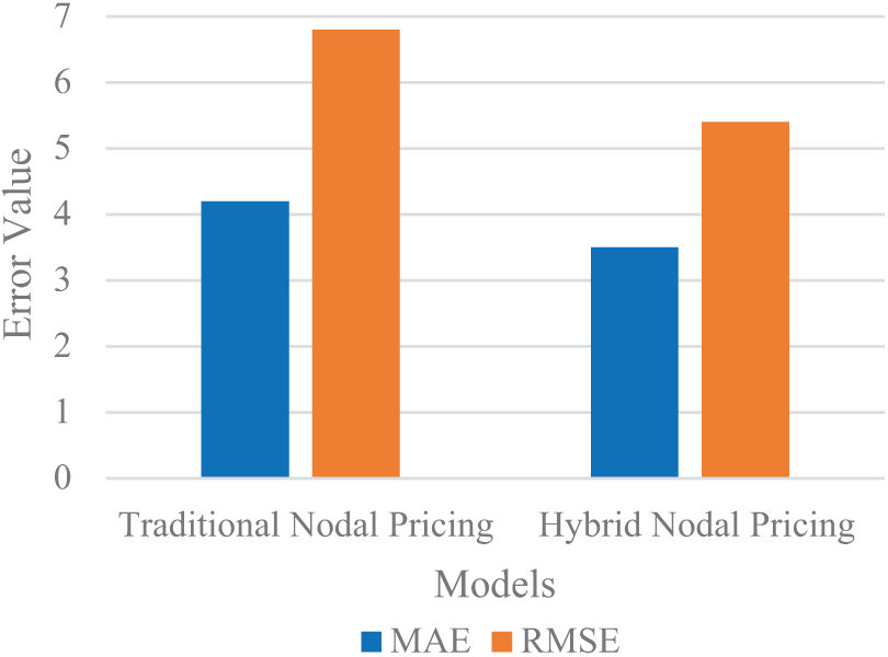
Figure 5: MAE and RMSE comparison
Table 3 presents the average line loading for both the HNPM and traditional models under various load and renewable energy scenarios. The HNPM demonstrates better management of line loading, with fewer instances of exceeding transmission line capacities.
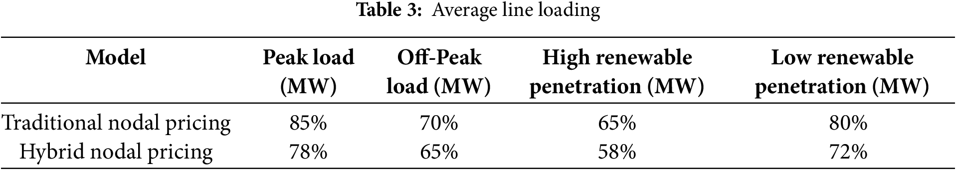
Fig. 6 illustrates average line loading under different conditions. The HNPM’s ability to maintain lower average line loading percentages indicates improved stability and efficiency in managing power flows. In figure, HRP is High Renewable Penetration whereas LRP is Low Renewable Penetration.
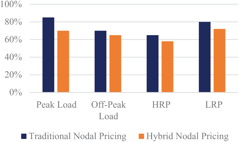
Figure 6: Line loading analysis
The system reliability is assessed by examining the number of instances where transmission line capacities are exceeded. The HNPM significantly reduces these occurrences compared to traditional models, enhancing overall network stability.
Fig. 7 shows graph comparing the frequency of transmission line exceedances for both models. The HNPM exhibits fewer exceedances, demonstrating its effectiveness in maintaining system reliability.
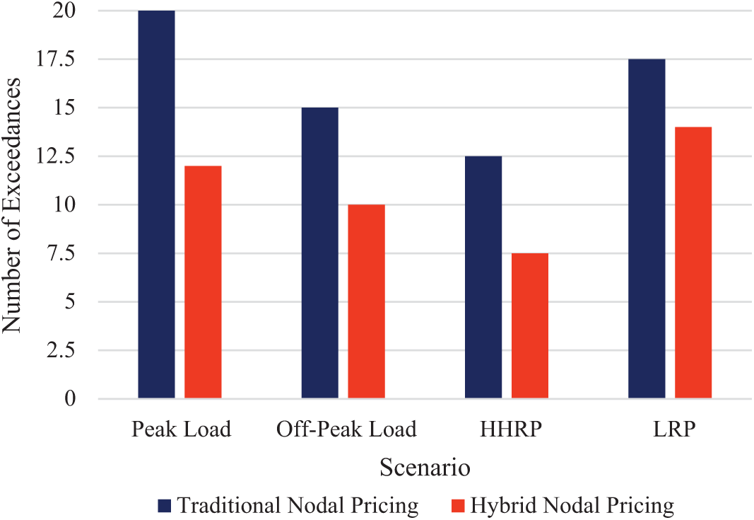
Figure 7: Reliability comparison
Tables 4 and 5 summarize the total operational costs, including generation, transmission losses, and congestion penalties, for the HNPM and traditional models across different scenarios.

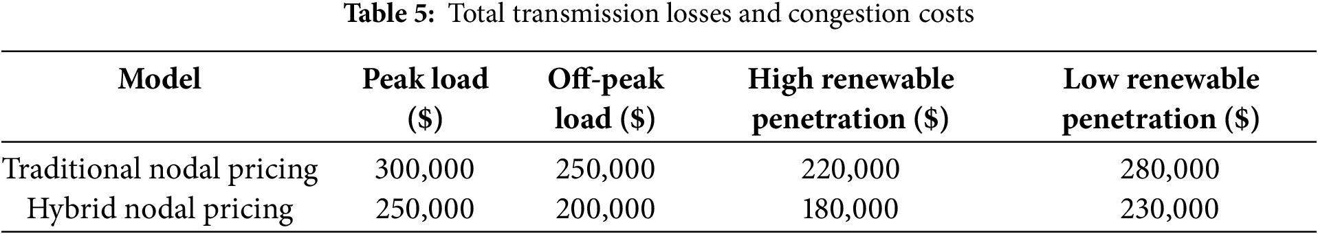
Fig. 8 presents a comparison of the total operational costs between the HNPM and traditional models. The HNPM results in lower overall costs, reflecting its enhanced efficiency in generation, transmission, and congestion management.
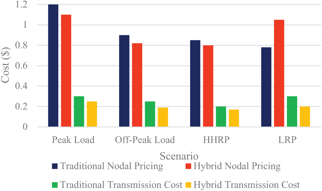
Figure 8: Total operational costs comparison
The results indicate that the Hybrid Nodal Pricing Model (HNPM) outperforms traditional nodal pricing methods in several key areas. The reduction in MAE and RMSE highlights the HNPM’s superior price prediction accuracy, which is critical for effective market operations and decision-making. This improved accuracy can lead to more efficient resource allocation and better financial outcomes for market participants [37].
In terms of network stability, the HNPM’s better management of line loading and reduced instances of capacity exceedances demonstrate its capability to enhance grid reliability. This is particularly important in maintaining system stability and avoiding costly disruptions.
Cost efficiency is another significant advantage of the HNPM. Lower total operational costs, including generation, transmission losses, and congestion penalties, underscore its effectiveness in optimizing the economic performance of the power system. By minimizing these costs, the HNPM contributes to a more economically sustainable and stable energy market [38].
Overall, the comprehensive evaluation of the HNPM through various metrics and scenarios confirms its potential to provide substantial improvements over traditional pricing models. The combination of accurate pricing, enhanced stability, and cost efficiency makes the HNPM a promising approach for modernizing power systems and addressing the challenges of dynamic and complex energy markets.
6.1 Improvement of MILP through Alternative Methods
Mixed-Integer Linear Programming (MILP) is a robust optimization technique widely used for solving linear problems involving both continuous and integer variables. However, MILP may face challenges when dealing with highly nonlinear problems or when rapid convergence is crucial. The Convergence Accelerated Decomposition Method (CADM) of Adomian offers promising enhancements in such scenarios.
The modified ADM introduces parameterized terms that control and pace the convergence of the ADM series. By optimizing these parameters to minimize squared residuals, the method ensures rapid and reliable convergence. Applying this approach to MILP could significantly reduce the computational time required for solving large-scale and complex problems. While MILP is designed for linear problems, real-world applications often involve nonlinearities. The CADM’s ability to handle highly nonlinear algebraic and differential equations suggests that integrating its principles could extend MILP’s applicability to a broader range of problems [39]. This integration would involve reformulating nonlinear components within the MILP framework using CADM techniques, thus improving solution accuracy and feasibility.
The CADM minimizes the number of iterations needed to reach a convergent solution, which is particularly beneficial for large-scale optimization problems. This efficiency can be leveraged in MILP to enhance its performance, especially in iterative methods like branch-and-bound or cutting planes, which are integral to solving MILP problems. One of the significant advantages of CADM is that it does not require numerical verification of results, thanks to the optimization of the embedded parameter. This feature ensures that the solutions generated are physically valid and reliable. Incorporating this aspect into MILP can improve the robustness of the solutions, particularly in applications requiring stringent feasibility and accuracy.
To integrate the Convergence Accelerated Decomposition Method with MILP, several steps can be considered. First, identify critical parameters within the MILP formulation that influence convergence and introduce parameterized terms as suggested by CADM. These parameters can be optimized using squared residual minimization to enhance convergence rates. Second, develop a hybrid optimization framework that combines the strengths of MILP and CADM, using MILP for linear components and employing CADM for nonlinear elements, ensuring seamless integration and improved overall performance. Third, enhance existing MILP algorithms with convergence control mechanisms inspired by CADM. This could involve modifying iterative processes to incorporate parameter adjustments dynamically, ensuring rapid and reliable convergence. Lastly, apply the modified MILP approach to various real-world problems, particularly those involving significant nonlinearity or requiring fast convergence, and validate the effectiveness through comparative studies, highlighting improvements in computational efficiency and solution accuracy [40].
6.3 Future Research Directions
Future research should focus on developing more efficient and scalable algorithms for nodal pricing, improving integration of renewable energy sources, and enhancing data analytics capabilities for real-time decision-making [38]. Exploring the use of artificial intelligence and machine learning can provide better predictions and optimizations. Furthermore, research into regulatory frameworks that support innovation while ensuring market stability and fairness is crucial. Advancements in these areas will pave the way for more efficient and reliable energy markets [41].
The assessment of the Hybrid Nodal Pricing Model (HNPM) highlights its effectiveness in improving various facets of power system management. Comprehensive simulations reveal that the HNPM provides more accurate pricing than traditional models. The notable decrease in Root Mean Squared Error (RMSE) and Mean Absolute Error (MAE) indicates the model’s enhanced capability to predict prices accurately, which is crucial for optimizing market operations and making well-informed decisions.
In terms of network stability, the HNPM shows notable improvements. It manages line loading more efficiently and reduces the frequency of transmission line exceedances, which helps maintain system reliability under diverse conditions, including varying load demands and renewable energy levels. This enhanced stability is critical for preventing disruptions and ensuring a consistent energy supply [41].
Cost efficiency is another significant benefit of the HNPM. The model leads to lower total operational costs, which include generation, transmission losses, and congestion penalties. By reducing these costs, the HNPM not only improves the economic performance of the power system but also supports a more sustainable and stable energy market.
Overall, the Hybrid Nodal Pricing Model represents a significant step forward in enhancing pricing accuracy and operational efficiency within power systems. Its ability to accurately forecast prices, bolster network stability, and reduce operational costs highlights its potential as a valuable asset in managing the complexities of modern energy markets. The positive outcomes from this assessment suggest that the HNPM could play a crucial role in advancing the development of more efficient and reliable power systems in the future.
Acknowledgement: The authors extend their appreciation to the Deanship of Scientific research at Zarqa University for supporting this research work. And we would like to express our sincere gratitude to all those who have contributed to the completion of this research. We extend our thanks to the department of Electrical Engineering at G. H. Raisoni University, Amravati, India for providing the necessary resources and support. Special thanks to Mukesh Kumar for their invaluable guidance and feedback throughout the project.
Funding Statement: The authors extend their appreciation to the Deanship of Scientific Research at Zarqa University, Zarqa, 13110, Jordan for funding this research work.
Author Contributions: All authors contributed significantly to this work. Ganesh Wakte conceived the original idea and designed the simulation framework. Mukesh Kumar performed the simulations and collected the data. Mohammad Aljaidi analyzed the results and drafted the manuscript. Ramesh Kumar and Manish Kumar Singla provided critical revisions and approved the final version of the manuscript. All authors reviewed the results and approved the final version of the manuscript.
Availability of Data and Materials: The datasets generated and analyzed during the current study are available from the corresponding author on reasonable request. Any requests for data and materials should be directed to Ganesh Wakte at ganesh.electrical@tgpcet.com.
Ethics Approval: Not applicable.
Conflicts of Interest: The authors declare no conflicts of interest to report regarding the present study.
References
1. Aravind VS, Anbarasi MS, Maragathavalli P, Suresh M, Suresh M. Smart electricity meter on real time price forecasting and monitoring system. In: 2019 IEEE International Conference on System, Computation, Automation and Networking (ICSCAN); 2019 Mar 29–30; Pondicherry, India. doi:10.1109/ICSCAN.2019.8878836. [Google Scholar] [CrossRef]
2. Stoft S. Power system economics: designing markets for electricity. Piscataway, NJ, USA: IEEE Press; 2002. p. 496. [Google Scholar]
3. Joskow PL, Tirole J. Transmission rights and market power on electric power networks. RAND J Econ. 2000;31(3):450. doi:10.2307/2600996. [Google Scholar] [CrossRef]
4. Borenstein S, Bushnell J, Stoft S. The competitive effects of transmission capacity in a deregulated electricity industry. RAND J Econ. 2000;31(2):294. doi:10.2307/2601042. [Google Scholar] [CrossRef]
5. Dashtdar M, Najafi M, Esmaeilbeig M, Bajaj M. Placement and optimal size of DG in the distribution network based on nodal pricing reduction with nonlinear load model using the IABC algorithm. Sādhanā. 2022;47(2):73. doi:10.1007/s12046-022-01850-1. [Google Scholar] [CrossRef]
6. Bhusan UK, Tomar RS, Narayankhedkar SK. Optimal transmission expansion planning in deregulated power markets using AI-enhanced cost-based pricing. In: Proceedings of the 2024 IEEE 13th International Conference on Communication Systems and Network Technologies (CSNT); 2024 Apr 6–7; Jabalpur, India. doi:10.1109/CSNT60213.2024.10545953. [Google Scholar] [CrossRef]
7. Kumar A, Kumar S, Sinha UK, Bohre AK, Saha AK. Optimal clean energy resource allocation in balanced and unbalanced operation of sustainable electrical energy distribution networks. Energies. 2024;17(18):4572. doi:10.3390/en17184572. [Google Scholar] [CrossRef]
8. Yang X, Wang X, Lu Z, Liang Z, Gu C, Li F. Distribution network tariff design: facilitate flexible resource under uncertain future energy scenarios. Energy Policy. 2024;188(2):114075. doi:10.1016/j.enpol.2024.114075. [Google Scholar] [CrossRef]
9. Zhang J, Sang L, Xu Y, Sun H. Networked multiagent-based safe reinforcement learning for low-carbon demand management in distribution networks. IEEE Trans Sustain Energy. 2024;15(3):1528–45. doi:10.1109/TSTE.2024.3355123. [Google Scholar] [CrossRef]
10. Ladwal S, Kumar A. Optimizing distributed generation placement and profit maximization in active distribution networks with harmonics: a GEPSO approach. Electr Power Compon Syst. 2024;2024(3):1–21. doi:10.1080/15325008.2024.2313587. [Google Scholar] [CrossRef]
11. Deihimi M, Rezaei N. Nodal price-based demand response management via orderly time-of-use strategy for an unbalanced isolated microgrid considering voltage stability constraints. Sustain Energy Technol Assess. 2024;65(1):103799. doi:10.1016/j.seta.2024.103799. [Google Scholar] [CrossRef]
12. Ran X, Suyaroj N, Tepsan W, Ma J, Zhou X, Deng W. A hybrid genetic-fuzzy ant colony optimization algorithm for automatic K-means clustering in urban global positioning system. Eng Appl Artif Intell. 2024;137(10):109237. doi:10.1016/j.engappai.2024.109237. [Google Scholar] [CrossRef]
13. Poggi A, Di Persio L, Ehrhardt M. Electricity price forecasting via statistical and deep learning approaches: the German case. AppliedMath. 2023;3(2):316–42. doi:10.3390/appliedmath3020018. [Google Scholar] [CrossRef]
14. Das R, Bo R, Chen H, Rehman WU, Wunsch D. Forecasting nodal price difference between day-ahead and real-time electricity markets using long-short term memory and sequence-to-sequence networks. IEEE Access. 2021;10:832–43. doi:10.1109/access.2021.3133499. [Google Scholar] [CrossRef]
15. Hogan WW. Electricity market design and zero-marginal cost generation. Curr Sustain Renew Energy Rep. 2022;9(1):15–26. doi:10.1007/s40518-021-00200-9. [Google Scholar] [CrossRef]
16. Chao HP, Peck S. A market mechanism for electric power transmission. J Regul Econ. 1996;10(1):25–59. doi:10.1007/BF00133357. [Google Scholar] [CrossRef]
17. Kirschen DS, Strbac G. Fundamentals of power system economics. Hoboken, NJ, USA: John Wiley & Sons, Inc; 2018. 344 p. [Google Scholar]
18. Oren SS. Economic inefficiency of passive transmission rights in congested electricity systems with competitive generation. Energy J. 1997;18(1):63–83. doi:10.5547/issn0195-6574-ej-vol18-no1-3. [Google Scholar] [CrossRef]
19. Bohn RE, Caramanis MC, Schweppe FC. Optimal pricing in electrical networks over space and time. RAND J Econ. 1984;15(3):360. doi:10.2307/2555444. [Google Scholar] [CrossRef]
20. Hogan WW. Markets in real electric networks require reactive prices. Energy J. 1993;14(3):171–200. doi:10.5547/issn0195-6574-ej-vol14-no3-8. [Google Scholar] [CrossRef]
21. Joskow PL. Capacity payments in imperfect electricity markets: need and design. Util Policy. 2008;16(3):159–70. doi:10.1016/j.jup.2007.10.003. [Google Scholar] [CrossRef]
22. Cramton P, Stoft S. The convergence of market designs for adequate generating capacity [Internet]. [cited on 2024 Nov 1]. Available from: https://ideas.repec.org/p/pcc/pccumd/06mdfra.html. [Google Scholar]
23. Woo CK, Horowitz I, Moore J, Pacheco A. The impact of wind generation on the electricity spot-market price level and variance: the Texas experience. Energy Policy. 2011;39(7):3939–44. doi:10.1016/j.enpol.2011.03.084. [Google Scholar] [CrossRef]
24. Green R. Nodal pricing of electricity: how much does it cost to get it wrong? J Regul Econ. 2007;31(2):125–49. doi:10.1007/s11149-006-9019-3. [Google Scholar] [CrossRef]
25. Bushnell JB, Stoft SE. Improving private incentives for electric grid investment. Resour Energy Econ. 1997;19(1–2):85–108. doi:10.1016/S0928-7655(97)00003-1. [Google Scholar] [CrossRef]
26. Joskow PL. Competitive electricity markets and investment in new generating capacity. In: Helm D, editor. The new energy paradigm. Oxford, UK: Oxford University Press (OUP); 2007. p. 76–121. doi: 10.1093/oso/9780199229703.003.0005. [Google Scholar] [CrossRef]
27. Hogan WW. Electricity market restructuring: reforms of reforms. J Regul Econ. 2002;21(1):103–32. [Google Scholar]
28. Newbery DM. Problems of liberalising the electricity industry. Eur Econ Rev. 2002;46(4–5):919–27. doi:10.1016/S0014-2921(01)00225-2. [Google Scholar] [CrossRef]
29. Oren SS. Ensuring generation adequacy in competitive electricity markets. In: Griffin JM, Puller SL, editors. Electricity deregulation. Chicago, IL, USA: University of Chicago Press; 2005. p. 388–414. doi: 10.7208/chicago/9780226308586.003.0011. [Google Scholar] [CrossRef]
30. Gan D, Feng D, Xie J. Electricity markets and power system economics. Boca Raton, FL, USA: CRC Press; 2014. 220 p. [Google Scholar]
31. Cramton P. Electricity market design: the good, the bad, and the ugly. In: Proceedings of the 36th Annual Hawaii International Conference on System Sciences; 2003 Jan 6–9; Big Island, HI, USA. doi 10.1109/HICSS.2003.1173866. [Google Scholar] [CrossRef]
32. Alghamdi FM, Edwards EC, Berglund EZ. Dynamic pricing framework for water demand management using advanced metering infrastructure data. Water Resour Res. 2024;60(9):e2023WR035246. doi:10.1029/2023WR035246. [Google Scholar] [CrossRef]
33. Turkyilmazoglu M. Nonlinear problems via a convergence accelerated decomposition method of adomian. Comput Model Eng Sci. 2021;127(1):1–22. doi:10.32604/cmes.2021.012595. [Google Scholar] [CrossRef]
34. Zhang Z, Chen Z, Gümrükcü E, Ji Z, Ponci F, Monti A. Advancing urban electric vehicle charging stations: ai-driven day-ahead optimization of pricing and Nudge strategies utilizing multi-agent deep reinforcement learning. eTransportation. 2024;22(2):100352. doi:10.1016/j.etran.2024.100352. [Google Scholar] [CrossRef]
35. Huang D, Deconinck G. Breaking borders with joint energy and transmission right auctions—assessing the required changes for empowering long-term markets in Europe. Energies. 2024;17(8):1923. doi:10.3390/en17081923. [Google Scholar] [CrossRef]
36. Ahunbay MŞ., Bichler M, Dobos T, Knörr J. Solving large-scale electricity market pricing problems in polynomial time. Eur J Oper Res. 2024;318(2):605–17. doi:10.1016/j.ejor.2024.05.020. [Google Scholar] [CrossRef]
37. Jiang Y, Dong J, Huang H. Optimal bidding strategy for the price-maker virtual power plant in the day-ahead market based on multi-agent twin delayed deep deterministic policy gradient algorithm. Energy. 2024;306:132388. doi:10.1016/j.energy.2024.132388. [Google Scholar] [CrossRef]
38. Lin X, Huang T, Wu H, Bompard EF, Wang B. Market zone configuration under collusive bidding among the conventional generators and renewable energy sources in the day-ahead electricity market. Electr Power Syst Res. 2024;232(6):110373. doi:10.1016/j.epsr.2024.110373. [Google Scholar] [CrossRef]
39. Meng W, Song D, Huang L, Chen X, Yang J, Dong M, et al. Distributed energy management of electric vehicle charging stations based on hierarchical pricing mechanism and aggregate feasible regions. Energy. 2024;291(5):130332. doi:10.1016/j.energy.2024.130332. [Google Scholar] [CrossRef]
40. Tostado-Véliz M, Horrillo-Quintero P, García-Triviño P, Fernández-Ramírez LM, Jurado F. Optimal sitting and sizing of hydrogen refilling stations in distribution networks under locational marginal prices. Appl Energy. 2024;374(1):124075. doi:10.1016/j.apenergy.2024.124075. [Google Scholar] [CrossRef]
41. Deng Z, Zhang Y, Guo F, Pan X, Zhu Z. Towards a low-carbon and low-risk community: risk-constrained optimization of energy pricing in electricity and gas networks with flexible carbon-responsive loads. J Clean Prod. 2024;437:140534. doi:10.1016/j.jclepro.2023.140534. [Google Scholar] [CrossRef]
Cite This Article
 Copyright © 2025 The Author(s). Published by Tech Science Press.
This work is licensed under a Creative Commons Attribution 4.0 International License , which permits unrestricted use, distribution, and reproduction in any medium, provided the original work is properly cited.
 Downloads
 Citation Tools