Multi-Timescale Optimization Scheduling of Distribution Networks Based on the Uncertainty Intervals in Source-Load Forecasting

1  Introduction

Distribution networks (DNs), as a key component of power systems, play a strategic role in energy transition and sustainable development [1]. Renewable energy-dominated power systems have evolved rapidly under the “dual carbon” goals of China, leading to increased penetration of renewable energy resources, flexible regulations, and increased diversity in power demand characteristics [2]. However, large-scale integration of renewable energy and flexible resources introduces significant uncertainties from generation and load perspectives, posing substantial challenges to the economic operation of power grids [3]. With the ongoing market-oriented reforms, dispatch strategy optimization, renewable energy utilization, and cost optimization have become critical issues for grid operators [4].

In renewable energy-based DN optimization studies, nonlinear programming can introduce complications, owing to large-scale decision variables, non-convex objective functions, and nonlinear constraints. These issues have been addressed by employing convex relaxation techniques, such as mixed-integer linear programming [5] and second-order cone programming [6], which reduce problem complexity through transformation but may compromise on the accuracy and global optimality of the solution. In recent years, distributed optimization algorithms have garnered increasing attention due to their flexibility and scalability. The alternating direction method of multipliers [7] enhances computational efficiency and ensures result accuracy through problem decomposition and node-level collaboration mechanisms, while consensus optimization [8] and Lagrangian dual relaxation [9] algorithms further improve overall performance and convergence speed by optimizing the iterative process. However, these approaches remain sub-optimal for upscaling due to their inability to lower computational costs and increase convergence rates, which are critical for real-time optimization.

Data-driven reinforcement learning (RL) techniques can identify complex dynamics by employing neural networks to capture multivariable and nonlinear relationships within a power system [10], thereby reducing the reliance on traditional power system models. Moreover, RL techniques can significantly enhance the computational efficiency and accuracy of power systems, providing a comprehensive solution for optimizing distributed renewable energy in modern DNs [11]. Researchers have employed various single-agent RL frameworks for optimizing DNs. For instance, the deep Q-network has been used for controlling grid voltage [12], the proximal policy optimization (PPO) algorithm has been used for scheduling time-coupled equipment (e.g., microturbines (MTs)) [13], and the deep deterministic policy gradient (DDPG) algorithm has been used for mitigating voltage limit violations caused by system uncertainties [14]. However, the limited scalability of these single-agent RL frameworks has prompted researchers to explore multi-agent (MA)-deep RL (DRL) frameworks, particularly those based on centralized training with decentralized execution (CTDE), which grants independent decision-making abilities to regulation equipment [15]. Li et al. [16] proposed a CTDE-based multi-agent DDPG (MADDPG) algorithm, which efficiently coordinates multiple distributed devices and addresses partial observability constraints, enhancing the flexibility and reliability of distribution systems; however, this algorithm shows limited adaptability under highly uncertain and dynamic environments. To address this limitation, Reference [17] introduced a multi-agent soft actor-critic (MASAC) algorithm, which enhances the ability of agents to cope with source-load uncertainty and complex power grids, thus significantly improving exploration capabilities, adaptability, and decision-making efficiency of distribution systems under complex environments. However, existing studies have not adequately addressed the impact of high uncertainty on the agent’s exploration capabilities and efficiency. These situations may expose agents to more unknown factors during the exploration process, affecting their learning speed and decision-making ability, and further restricting their ability to adapt and optimize performance in dynamic environments.

It is crucial to establish effective modeling and processing methods, such as scenario-based, chance-constrained programming, robust optimization, and interval optimization methods, to address the uncertainties in renewable energy-based DNs, particularly those arising from environmental and climate variations. Stochastic optimization methods generate multiple scenarios to simulate the impact of uncertain factors and provide their probability distribution in energy generation [18]. However, these methods struggle to balance computational efficiency with accuracy [19]. Robust optimization methods generate worst-case scenarios, based on the possible variations in uncertain factors, to ensure the feasibility of optimization strategies within the range of parameter perturbations [20]. However, these traditional methods primarily rely on boundary information (minimum and maximum values) of uncertain quantities, often leading to overly conservative optimization results [21]. Although studies have reduced the conservativeness of robust optimization through spatiotemporal correlation [22] and probability distribution [23], these improvements increase the complexity of the optimization model, limiting its application in large-scale systems. Interval optimization methods describe uncertain values as interval numbers and use interval arithmetic to determine the optimal interval [24]. Compared to stochastic optimization, interval optimization makes DNs efficient and less conservative. However, the effectiveness of interval optimization is closely associated with selecting the appropriate range of interval variables, which is crucial for achieving optimal results. In particular, obtaining reasonable interval variables is critical in scenarios with high source-load uncertainty.

Despite improving the economic efficiency and safety of power grid operations under source-load bilateral uncertainty, the existing DN optimization methods exhibit two significant limitations. First, the high uncertainty environment severely restricts the exploration efficiency and learning speed of optimization algorithms, leading to increased computational complexity and prolonged training cycles. Second, the existing methods fail to adequately consider the dynamic characteristics of source-load prediction errors across different timescales, resulting in overly conservative uncertainty intervals that reduce scheduling accuracy and efficiency.

In this study, we propose a multi-timescale optimal scheduling method that aims to enhance scheduling flexibility, accuracy, and computational efficiency by addressing the uncertainties in source-load prediction. The main contributions of this study are summarized as follows:

(1)   The novel multi-timescale optimization scheduling method incorporates source-load forecast uncertainty intervals by analyzing the flexibility requirements at multiple timescales (day-ahead, intra-day, and real-time) to optimize grid operations, thereby ensuring economic efficiency.

(2)   The improved SAC algorithm dynamically adjusts the weight of entropy in policy optimization through a self-regulating temperature coefficient and improves the agents by reducing unnecessary explorations.

(3)   The CTDE-based MASAC framework effectively reduces the decision-making time in the optimization process, ensures real-time scheduling, and significantly improves the overall system efficiency.

2  Optimal Dispatch Strategy Based on the Uncertainty Intervals of Source-Load Forecast

2.1 Analysis of Source-Load Uncertainty and Grid Flexibility

The forecasting timescale plays a crucial role in determining the accuracy of source-load predictions while addressing uncertainty in DNs. The extent of uncertainty errors varied across different forecasting timescales, significantly affecting source-load predictions [25] (Fig. 1). Generally, day-ahead forecasting utilizes a 1-h timescale, which is influenced by various uncertainty factors, like long-term weather variations, equipment degradation or potential malfunctions, and consumer electricity demand variations, resulting in increased forecasting errors. Conversely, intra-day forecasting adopts <1-h timescales, which are influenced by short-term factors, such as transient weather changes, temporary equipment failures, and short-term demand fluctuations, resulting in enhanced accuracy and reduced uncertainty intervals. Real-time forecasting employs even shorter timescales (~5 min) to achieve superior precision and predictive confidence intervals.

Figure 1: Comparison of predicted data across different timescales

2.1.1 Characterization of Uncertainty Intervals in Source-Load Forecasting

The variability range of uncertain variables significantly influences the optimization performance of power grid systems. In this study, we utilized the probability box (p-box) theory to accurately delineate the appropriate uncertainty intervals for source-load forecasting [26].

(1)   Gaussian distribution assumption

The source-load prediction error is often represented as a normal distribution, owing to the central limit theorem, which states that when errors arise from numerous independent random factors, their probability distribution tends to be normal. This assumption has been widely validated in load forecasting studies. The relative prediction error data for Liaoyang, China (2022) conformed to a normal distribution (Fig. 2a). The statistical histogram aligned well with the probability density and cumulative probability functions of the fitted normal distribution, indicating that load prediction errors can be represented as a normal distribution, laying the foundation for subsequent statistical analysis and model optimization. Additionally, when the sample size is sufficiently large, the prediction errors of wind or photovoltaic (PV) power outputs tend to conform to a normal distribution, despite the influence of various factors [27]. Although the prediction errors of wind power can exhibit various distribution types, like beta, Cauchy, or Laplace distributions, their overall concentration trend can be successfully captured by a normal distribution (Fig. 2b). Similarly, the prediction errors of PV power, influenced by the stochastic and independent variations in solar radiation intensity, can be conventionally represented by a normal distribution [28] (Fig. 2c). Based on the aforementioned theoretical and empirical analyses, this study utilizes a normal distribution model to characterize source-load prediction errors.

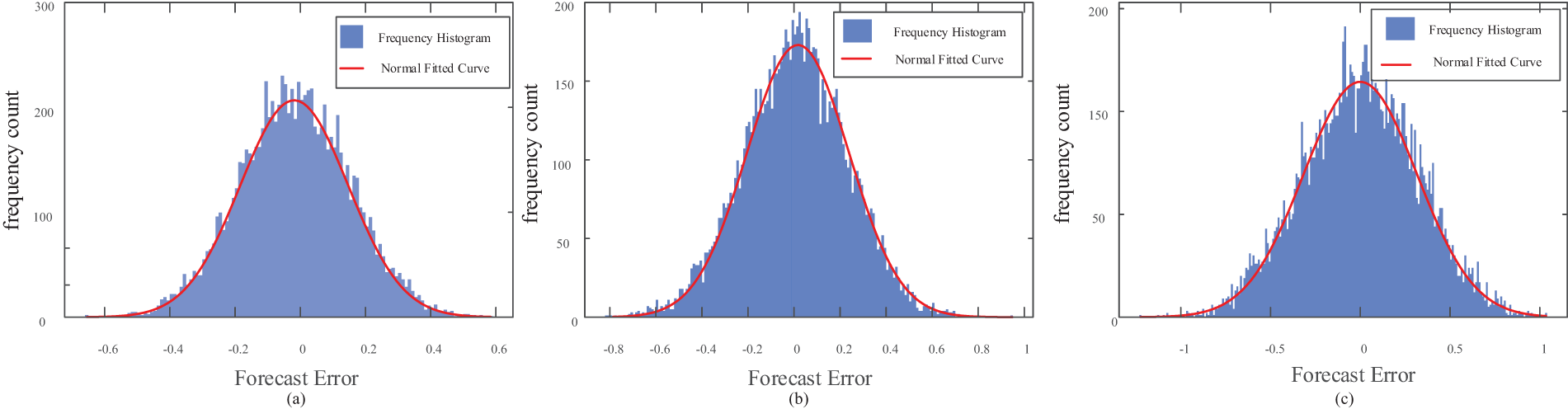
Figure 2: Distribution of source-load prediction errors

(2)   P-box-based interval extraction

The p-box theory represents uncertainty as interval-based probability distributions, yielding precise and conservative estimates. Particularly in cases with limited data availability or expert input, the p-box theory provides a validated uncertainty range for extracting source-load intervals. It accurately characterizes uncertainty, manages nonlinear and complex system dynamics, and offers a reliable foundation for informed decision-making.

The interval characterization was performed as follows: For a given scheduling day, wind turbine (WT) and PV output, as well as flexible load (FL) demand was predicted using predictive algorithms. The resulting values, denoted as P~N,t, form the deterministic component of the random variable, τ, within the p-box theory framework. The uncertainty of the random variable was represented as the forecast error, eN,t. The p-box parameters, based on historical data analysis, can be used to define the upper (F⌢N,t(τ)) and lower (F˘N,t(τ)) limits for the cumulative probability distribution function as interval boundaries. Source load-related forecast errors can be represented by a normal distribution. Consequently, the mean (μN,t) and standard deviation (σN,t) vary within a specified range, denoted by μN,t∈(μ˘N,t,μ⌢N,t) and σN,t∈(σ˘N,t,σ⌢N,t), respectively. The boundaries of the cumulative probability distribution function, corresponding to the probability distribution parameters of the forecast error, can then be defined as

{FN1,t(τ)∼N(μ˘N,t(σ⌢N,t)2)FN2,t(τ)∼N(μ˘N,t(σ˘N,t)2)FN3,t(τ)∼N(μ⌢N,t(σ˘N,t)2)FN4,t(τ)∼N(μ⌢N,t(σ⌢N,t)2)(1)

with a confidence level of β=0.9, and the upper and lower boundary quantiles set at 95% and 5%, respectively, implying that FN1,t(e˘N,t)=0.05 and FN4,t(e⌢N,t)=0.95. This configuration facilitates the calculation of the predictive interval,

[P˘N,t,P⌢N,t]=[P~N,t+e˘N,t,P~N,t+e⌢N,t](2)

After acquiring the forecasted values for PV, WT, and Load, the uncertainty intervals were assessed using the p-box theory. As indicated in [26], the net load (NL) was computed as follows: PNL,t=PL,t−(PWT,t+PPV,t). The NL forecasting error, eNL,t, could then be deduced from the forecast errors of PV, WT, and Load. The uncertainty interval for the NL was then defined as

[P˘NL,t,P⌢NL,t]=[P~NL,t+e˘NL,t,P~NL,t+e⌢NL,t](3)

2.1.2 Incorporating Flexibility Requirements for Scheduling Intervals

Flexibility demand highlights the need for an adaptable grid dispatch to address the uncertainties in the source and load forecasts of power systems. Conversely, flexibility supply represents the capacity and availability of resources within a power system to ensure adaptability. Adequate flexibility supply enables the maintenance of flexibility balance across various temporal, spatial, and scale dimensions, ensuring that flexibility always exceeds demand. In multi-timescale optimal dispatch, especially under forecast uncertainties, it is essential to anticipate and meet future flexibility demands during the preceding scheduling stage. By securing sufficient dispatch supply capacity or flexible reserve capacity at an earlier stage, the power system can maintain a flexibility balance and sustain supply-demand equilibrium, even amid significant fluctuations in source-load forecasts in subsequent phases.

The range of uncertain demand capacity in a power system can be evaluated by calculating the uncertainty intervals in source-load forecasting along with the predicted NL values. This aids in defining the extent of flexibility supply capacity. Meanwhile, the flexibility demand capacity can be evaluated by examining the changes in NL forecasts between preceding and current time points, along with their associated prediction intervals. The variation in the predicted NL was calculated using the following equation:

ΔPNL,t=PNL,t−PNL,t−1(4)

where PNL,t and PNL,t−1 represent the NL power at the current and preceding time points, respectively and ΔPNL,t indicates the change in NL and serves as a measure of the flexibility demand. Flexibility equilibrium is achieved when the flexibility supply capacity, ΔPR,[t−1,t]≥ΔPNL,t, without considering the prediction uncertainty intervals.

Since NL forecasts are inherently directional, the flexibility of the power system also follows a directional trend (Fig. 3), involving two key scenarios: PNL,t≥PNL,t−1 and PNL,t<PNL,t−1. With the incorporation of uncertainty intervals into the NL forecasts, it is essential to determine the flexibility demand capacity range along with the overall flexibility demand, as follows:

[ΔP˘NL,t,ΔP⌢NL,t]=[P˘NL,t−P⌢NL,t−1,P⌢NL,t−P˘NL,t−1](5)

Figure 3: Flexibility demand diagram

The constraints on flexibility supply capacity can then be determined using Eq. (5) as

ΔP⌢R,t≥ΔP⌢NL,t(6)

ΔP˘R,t≤ΔP˘NL,t(7)

where a positive value indicates the potential to increase discharge capacity, while a negative value indicates the ability to reduce discharge and charge capacity.

When PNL,t>PNL,t−1, the upward flexibility supply capacity (|ΔP⌢R,t|) is notably larger (Fig. 3). Conversely, when PNL,t<PNL,t−1, the downward flexibility reserve capacity requirement (|ΔP˘R,t|) is significantly larger. In scenarios, where PNL,t=PNL,t−1, it follows that PNL,t=PNL,t−1, equivalent to the NL forecast error eNL,t. The constraints on the flexibility reserve capacity range can be determined through the flexibility demand interval and the flexibility supply capacity.

2.2 Multi-Agent RL Algorithm Based on Uncertainty Intervals in Supply and Load

RL comprises three key components: the agent, environment, and reward. The agent interacts with its environment through trial and error, aiming to maximize the cumulative reward. RL tasks can be modeled using a Markov decision process, which is characterized by four elements: state space (S), action space (A), state transition probability (P), and reward space (R) [29].

In this study, we employed a CTDE framework to optimize the dispatch of DNs handling large datasets. This approach extends single-agent DRL algorithms to multi-agent environments, allowing multiple agents to optimize the active DNs, while improving computational efficiency [30].

2.2.1 Enhanced SAC Algorithm

The SAC algorithm was used to develop a control model for active DNs and establish a system operation control strategy. During training, the SAC algorithm designs policies by balancing expected returns with information entropy, thereby preventing the emergence of suboptimal global solutions [29]. This framework enables agents to comprehensively understand source-load uncertainties, enhancing the system’s ability to optimize globally and adapt to these uncertainties. Furthermore, this algorithm incorporates agents’ action entropy into the value function, thereby encouraging exploration and improving stability. The action entropy of the agents can be defined as

H(πφ(∙|st))=Ea∼πφ(∙|st)[−log⁡πφ(at|st)](8)

where φ represents the network parameters of the policy π. Action entropy measures the uncertainty in action selection, allowing the policy to produce a diverse range of actions during iterative training. This ensures that the agent can explore a broader spectrum of potential actions, minimizing the likelihood of neglecting potentially beneficial decisions. The discounted cumulative reward function (J) of the SAC and the optimal policy (π∗) were defined as follows:

J=∑t=0TE(st,at)∼ρπ[r(st,at)+αH(πφ(∙|st))](9)

π∗=arg maxπφ⁡∑t=0TE(st,at)∼ρπ[r(st,at)+αH(πφ(∙|st))](10)

where π represents the agent’s action policy (probability distribution of action selection); st denotes the current environmental state encountered by the agent; at represents the action derived from the policy; r(st,at) indicates the reward value provided by the environment to the agent; (st,at)∼ρπ represents the action trajectory of the policy; and α represents the temperature coefficient of the action entropy, which determines the impact of action entropy on the reward.

(1)   Enhanced temperature coefficient update

The temperature coefficient adjusts with changes in environmental uncertainty, and its size significantly impacts the model’s capability to explore uncertainties, influencing exploration behavior and optimization efficiency during training. In this study, we proposed an automatic temperature coefficient adjustment method to refine uncertainty learning and minimize redundant exploration. This approach dynamically adjusts the agent’s temperature coefficient based on the level of environmental uncertainty. The update calculation for each step of the optimization process can be expressed as

{αt=α+ηt(eN,t/P~N,t)α¯t=αt−λαE(st,at)∼ρπ[−α log(π(at|st)−atH0](11)

The kt∈[0,1] coefficient assesses the level of scheduling uncertainty in an environment at a given time and is primarily influenced by the predicted power output and the magnitude of forecast errors. The ηt parameter quantifies uncertainty and is determined by historical prediction error data and the system’s environmental sensitivity. This approach ensures that the influence of action entropy on the reward function modifies according to the degree of environmental uncertainty.

(2)   SAC network

SAC employs an actor network to model the action policy (πφ) and a critic network to evaluate the derived policy using a value function. In this study, the parameters of both the actor and critic networks were updated through gradient-based backpropagation to optimize the operating policy and the Q-value function. The state value functions in SAC were defined as

Vθi(st+1)=Eat∼π[Qθi(st+1,at+1)−α ln πφ(at|st)](12)

where Est+1∼ρπ[V(st+1)] represents the sum of expected values across all the states (st+1) along the ρπ trajectory. The θi parameter was updated by minimizing the soft Bellman residual as

JQ(θi)=E(st,at)∼D12(Qθi(st,at)−(r(st,at)+γEst+1τπ(st,at)[Vθ¯i(st+1)]))2](13)

where D represents the replay buffer used to update the sample set, which generally stores tuples of four elements (st,at,rt and at′). The term Vθ¯(st+1) denotes the updated state value function of the critic network, while θ¯ represents the parameters of the target soft Q-function.

The policy parameters, φ, were updated using the Kullback–Leibler (KL) divergence as

Jπ(φ)=Est∼D[DKL[[πφ(∙|st)]‖exp(1αQθ(st∙))Zθ(st)]](14)

where Zθ(st) denotes the distribution function used for normalization, while DKL[||] represents the KL divergence, which quantifies the distance between two distributions. The policy parameters, φ, can be learned by minimizing this equation. Reparameterization was applied to the policy outputs to reduce variance in the estimates, as follows:

Jπ(φ)=Est∼D,t∼N[αlog⁡(πφ(fφ(εt,st)∣st))−Qθ(st,fφ(εt,st))](15)

where fφ(εt,st) represents a sample from the probability distribution of the agent’s action (at) and εt∼N(0,I) represents a noise term.

To ensure stable operation of the SAC algorithm after every critic network parameter adjustment, the target critic network was subjected to a soft update, as follows:

θ¯i=δθi+(1−δ)θ¯i(16)

where δ denotes the hyperparameter for the soft update of the target network in the control system. The specific algorithmic framework is illustrated in Fig. 4.

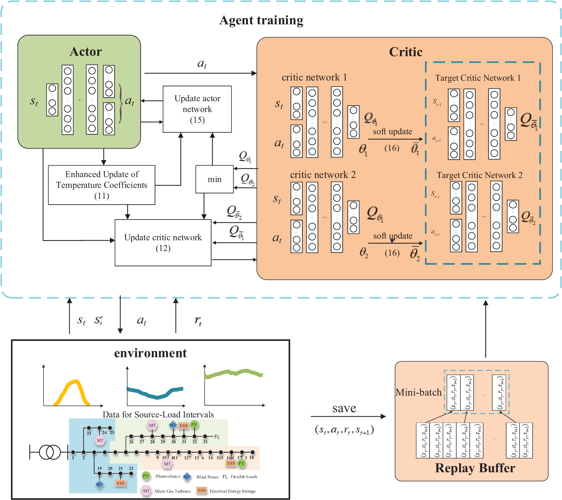
Figure 4: An optimized scheduling framework based on an improved SAC algorithm

2.2.2 Design of CTDE-Based MASAC Network Model

The multi-agent training framework utilizes the CTDE framework to enhance efficacy. To ensure that each agent remains stable during the training process, the critic network incorporates additional data from the observations and actions of other agents. However, during execution, the actor network makes decisions based solely on the agent’s private observations. The CTDE framework is illustrated in Fig. 5.

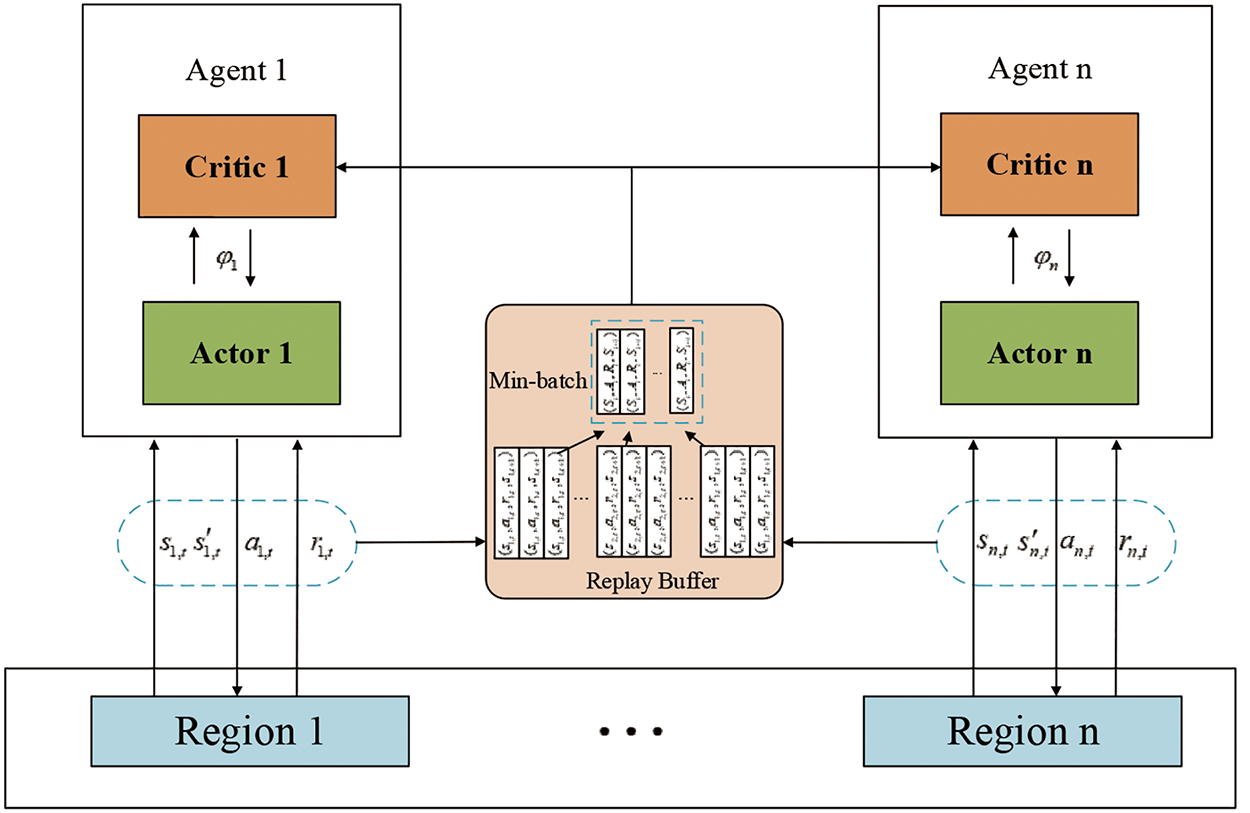
Figure 5: Training diagram for multi-agent RL

During the training process, the actions, states, and rewards of each agent are stored in a replay buffer (D), which is utilized by the critic network to access observations and actions from other agents, enabling neural network updates. Consequently, the experience tuples are expanded to encompass the elements of all the agents: (St,Ar,Rt,St′), where St=(s1,t,s2,t,⋯,sn,t), An=(a1,t,a2,t,⋯,an,t), Rt=(r1,t,r2,t,⋯,rn,t), and St′=(s1,t′,s2,t′,⋯,sn,t′).

Within an environment, each agent, m (m∈[1,2,⋯,n]), possesses an actor network πm∈{π1,⋯,πn}, with its corresponding parameters denoted as φm∈{φ1,⋯,φn}. The actor network parameters (φ) for agent m were determined according to the CTDE framework and SAC algorithm, as follows:

Jπm(φm)=Esm,t∼D,m∼N[α log(πφm(fφm(εt,sm,t)∣sm,t))−Qθm(St,At)](17)

Each agent has an independent actor-critic network, generating distinct actions (at) based on its unique observed state (st). Unlike the actor network, the critic network is capable of accessing the states (St) and actions (At) of all the agents from a shared experience replay buffer (D). This approach enables each agent to adapt effectively to a multi-agent collaborative environment. The parameter update for the critic network, denoted as θm, is formulated as

JQm(θm)=E(st,at)∼D12(Qθm(St,At)−(rm(st,at)+γESt+1τπ(St,St)[Vθ¯(St+1)]))2](18)

V(St+1)=Eat∼π[Qθ¯(St+1,At+1)−α ln πφ¯(am,t+1|sm,t+1)](19)

In the experience replay buffer (D), random sampling was used to obtain a fixed batch of sample pairs, JQm(θm), for approximate calculation. For agent m, the observed value of the next state (sm,t+1) was fed into the target actor network (πφ), and the action probability distribution was sampled to determine the agent’s next action (am,t+1). This process ensures a more stable and consistent learning trajectory by utilizing both the primary and target networks to decouple the action selection and value evaluation phases.

2.3 Multi-Timescale Scheduling Framework Based on Source-Load Uncertainty Intervals

In this study, we employed a multi-time-scale optimization strategy for DNs to manage the fluctuations in source-load forecasting uncertainties across multiple timescales: day-ahead, intra-day, and real-time stages. An enhanced MASAC algorithm was employed to centrally train agents across different timescales, facilitating the development of an efficient DN optimization and control strategy. The training dataset was constructed based on the historical data, incorporating renewable energy and load data into the environmental model. The DN operational data served as the state input for the agents. The actions generated by the agents were transformed into control commands, and the rewards were calculated according to a predefined reward function. A comprehensive overview of the scheduling framework is depicted in Fig. 6.

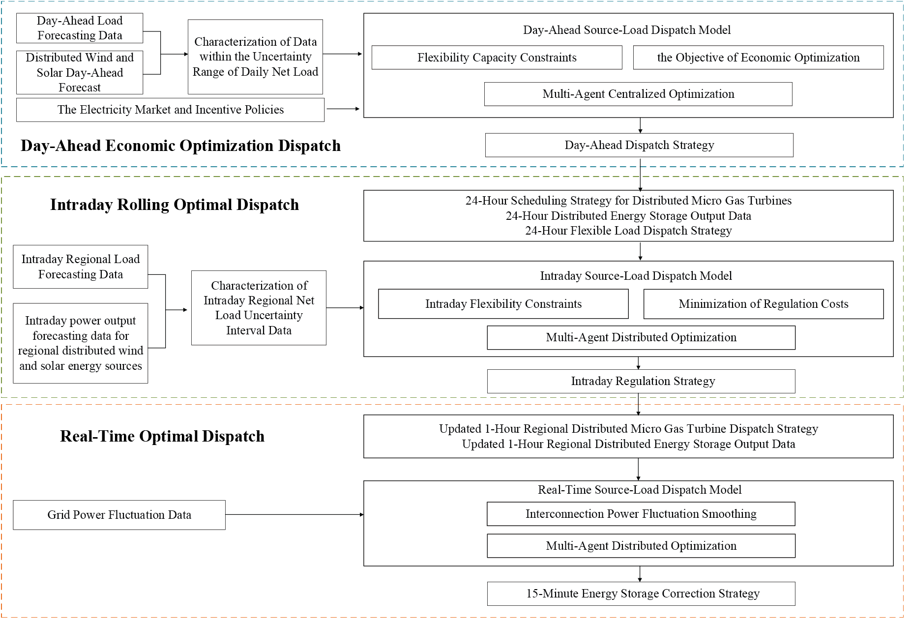
Figure 6: Multi-timescale optimal scheduling framework

In the day-ahead stage, uncertainties primarily stem from deviations in medium- to long-term weather forecasts and random load variations. Based on historical prediction error data, the p-box theory can determine the potential ranges and probability distributions of prediction errors for PV power, wind power, and load. Since day-ahead forecasts are generally updated once per day, their error ranges remain relatively stable, encompassing uncertainties over an extended period. Consequently, day-ahead optimization can provide 24-h generation schedules and reserve capacities; however, its inability to capture short-term variations may lead to conservative and economically inefficient outcomes. Day-ahead optimization provides the basis for intra-day and real-time optimizations, ensuring the reliability and economic efficiency of the system over an extended period. The agent operates at a 1-h timescale, employing centralized optimization to maximize economic efficiency in daily power system operations. The uncertainty intervals of source-load forecasts are incorporated at this stage to generate 24-h dispatch strategies, including scheduling of distributed MTs, optimizing energy storage systems (ESSs), regulating flexible loads, and maintaining a degree of robustness.

In the intra-day stage, uncertainties primarily stem from short-term meteorological changes, such as cloud movement and wind speed fluctuations, as well as random load variations. As forecasts are updated every 15 min to 1 h at this stage, the p-box effectively captures short-term fluctuations to generate more accurate error intervals and probability distributions, enhancing uncertainty descriptions for rolling optimization. This ensures that generation schedules and reserve capacities are dynamically modified to optimize the output of controllable resources, like ESSs and MTs, based on uncertainties. Compared to the day-ahead stage, the intra-day stage has higher data update frequency and more flexible optimization strategies, which enhance the trade-off between economic efficiency and system reliability. Operating on a 15-min timescale, this approach employs offline centralized training and online decentralized execution for decision-making. It primarily revises day-ahead decisions based on intra-day power generation and load variations, generating 1-h dispatch strategies for MTs and ESSs and ensuring regional robustness and economic efficiency.

3  Multi-Timescale Optimal Control Model Based on the Uncertainty Intervals of Source-Load Forecasting

The multi-timescale optimization and control model, incorporating the uncertainty intervals of source-load forecasting, aims to reduce grid generation costs, enhance local renewable energy integration, and mitigate source-load power fluctuations. Additionally, the model integrates flexibility requirements arising from source-load forecasting uncertainties at each timescale to ensure an adequate capacity for flexibility.

3.1 Day-Ahead Economic Optimal Control Model

In the day-ahead stage, a centralized optimization strategy is utilized to achieve optimal DN scheduling and maximize economic efficiency for the grid’s 24-h operation. This method ensures the grid’s safety and economic efficiency by regulating MTs, distributed ESSs, and FLs on an hourly basis.

3.1.1 Objective Function of Day-Ahead Optimization

The latest economic optimization scheduling aims to reduce the daily DN operation costs by assuming the complete integration of WT and PV power generation. The optimization objective is defined as

C1=∑t=1T[Cgrid(t)+Closs(t)+CESS(t)+CFL(t)+∑X∈ΩXCpunishX(t)](20)

where T represents the number of control periods within a regulation cycle and the terms Cgrid(t), Closs(t), CESS(t), CFL(t), and CpunishX(t) represent DN generation cost, DN active power loss cost, ESS regulation cost, FL regulation cost, and penalty cost associated with Project X constraints (ΩX), respectively, at time t. The constraints (ΩX) for optimal power system scheduling include state of charge (SOC) constraints for ESSs, power line constraints, and day-ahead flexibility capacity constraints for MTs and ESSs. The specific formulas for each cost variable in Eq. (20) are as follows:

Cgrid(t)=λgrid|Pgrid(t)|+λMT|PMT(t)|(21)

Closs(t)=λlossPloss⋅grid(t)(22)

CESS(t)=λESS[ηchaPESScha(t)+PESSdis(t)ηdis](23)

CFL(t)=∑i=1nFLλFL|PFL,iori(t)−PFL,i(t)|(24)

CpunishX(t)={ω1X[Xmin−X(t)]0ω2X[X(t)−Xmax]X(t)<XminXmin≤X(t)≤XmaxX(t)>Xmax(25)

3.1.2 Constraints

The constraints for the optimization of power system scheduling intervals are DN branch power flow constraints, power grid voltage magnitude constraints, MT output constraints, FL constraint, line transmission power constraint, and flexibility capacity constraint.

(1)   Branch power flow constraints in DNs

{∑j∈M(i)Pij,t−∑k∈N(i)(Pki,t−Iki,t2Rki)=Pi,tinj∑j∈M(i)Qij,t−∑k∈N(i)(Qki,t−Iki,t2Xki)=Qi,tinjVj,t2=Vi,t2−2(Pij,tRij+Qij,tXij)+Iij,t2(Rij2+Xij2)Iij,t2Vi,t2=Pij,t2+Qij,t2Pi,tinj=PPVi,t+PWTi,t+PMTi,t+PESSicha(t)+PESSidis(t)−PFL,i(t)−Pi,tLoadQi,tinj=QPVi,t+QWTi,t−QFL,i(t)−Qi,tLoad(26)

where Pij,t and Qij,t represent the active and reactive power at the injection node i, respectively.

(2)   Voltage magnitude constraints in a power grid

V_j≤Vj,t≤V¯j,(27)

where V_j and V¯j denote the upper and lower limits of the voltage magnitude at node j, respectively.

(3)   MT output constraints

{P_MT≤PMTi,t=PMTi,t−1+ΔPMTi,t≤P¯MTΔP_MT≤ΔPMTi,t≤ΔP¯MT(28)

Q_MT≤QMTi,t≤Q¯MT(29)

where ΔPMTi,t and QMTi,t denote the active power variation and reactive power output of MT i, respectively, during the time period t.

(4)   ESS charging/discharging power and capacity constraints

PESScha(t)⋅PESSdis(t)=0(30)

{PESScha(t)≤PESScha.maxPESSdis(t)≤PESSdis.max(31)

At any time, the ESS can be in a charging or discharging state at a specified maximum power capacity [31].

{SOC(t)=SOC(t−1)+ηchaPESScha(t)SESS+PESSdis(t)ηdisSESSSOCmaxmin(32)

(5)   FL constraint

The user side consists of various types of FLs, including interruptible loads and transferable loads. Interruptible loads can function as virtual power sources and can adopt control strategies similar to those used for distributed energy resources. Contrastingly, shiftable loads represent a specialized form of transferable loads, characterized by their ability to alter the timing of energy usage through price adjustments or incentive measures without reducing the total demand load. In this study, we examined shiftable loads to analyze FL regulation strategies in DNs. For this, we considered the invariance of the total load over the control cycle as the principal constraint, expressed as

∑t=0TPFL,i(t)=∑t=0TPFL,iori(t)(33)

Additionally, during each control period, the adjustable capacity of transferable loads was subject to certain constraints, defined by upper and lower power limits.

PFL,imin(t)≤PFL,i(t)≤PFL,imax(t)(34)

(6)   Line transmission power constraint

Pij,t2+Qij,t2≤Sij2(35)

(7)   Flexibility capacity constraint

In the day-ahead stage, the scheduling strategy is adjusted using distributed MTs and ESSs. Therefore, the reserve capacity during this phase is derived from the reserve capacities of MTs and ESSs, expressed as

ΔP⌢ESSi,R,t=PESScha.max−PESSi(t),(36)

ΔP⌢MTi,R,t=ΔP¯MT−ΔPMTi,t(37)

ΔP⌢ESSi,R,t+ΔP⌢MTi,R,t≥ΔP⌢i,R,[t−1,t](38)

where ΔP⌢ESSi,R,t and ΔP⌢MTi,R,t represent the upward flexibility capacity of ESSs and MTs, respectively, in region i during the time period t. Their sum must be equal to or greater than the required upward reserve capacity.

ΔP⌢ESSi,R,t=PESScha.max−PESSi(t)(39)

ΔP⌢MTi,R,t=ΔP¯MT−ΔPMTi,t(40)

ΔP⌢ESSi,R,t+ΔP⌢MTi,R,t≥ΔP⌢R,[t−1,t](41)

where ΔP˘ESSi,R,t and ΔP˘MTi,R,t denote the downward reserve capacity constraints for ESSs and MTs, respectively, in region i during the time period t. The sum of these constraints must be less than or equal to the downward reserve capacity.

3.1.3 Day-Ahead Scheduling Model

(1)   State space

The state space (S) for the k-th agent within region k was constructed by selecting the active power output of k MT units (PMT,t,k), forecasted PV output (PPV,t,k), forecasted WT output (PWT,t,k), forecasted load (Pload,t), SOC at t − 1 (SOCk(t−1)), and electricity purchase price from the distribution grid λgrid(t) as the state variables, expressed as

S={PMT,t,k,PPV,t,k,PWT,t,k,Pload,t,λgrid(t),SOCk(t−1)}(42)

(2)   Action space

Since day-ahead regulation targets the ESSs, distributed generators, FLs, and PV and WT power system inverters, its action space (A) is defined as follows:

Ahour={PESS(t)|t∈[1,T−1],PMT(t)|t∈[1,T−1],PFL,i(t)|i∈[1,nFL],t∈[1,T]}(43)

(3)   Reward function

The SAC policy network aims to derive strategies that maximize the reward. Therefore, to minimize the objective function, the reward values (R) were set as the negative of the original objective function, as follows:

R1=−C1(44)

3.2 Intra-Day Optimization and Control Model

Active DNs are divided into several autonomous regions based on geographical conditions and regional consumption patterns. Each autonomous region is equipped with a regional agent that issues dispatch instructions to the controllable devices within its area. These agents utilize ultra-short-term forecasts of renewable energy generation, FL, and device status within the region to optimize their operations [32].

The regional agents employ CTDE-based neural networks, wherein the network parameters for each agent are obtained through centralized training, following which the trained agents are deployed for distributed control. In the t-th scheduling interval, regional agent (k) employs a policy network to determine a dispatch decision (ak,t) based on the regional state (Sk,t) and receive a regional reward (Rk,t). Since intra-day optimization involves adjustments based on day-ahead optimization, its scope of control is relatively limited. During the day-ahead optimization process, a certain control margin is reserved within each region to adequately address the challenges and fluctuations arising from intra-day variations in source-load forecast data.

3.2.1 Objective Function of Intra-Day Optimization

The intra-day optimization strategy refines the day-ahead grid plan to mitigate challenges associated with energy supply and renewable energy deficits, which arise from forecasting errors. By adjusting MTs and ESSs, this strategy maintains the grid’s supply-demand equilibrium, enhances local renewable energy integration, upholds the grid’s economic efficiency, and ensures sufficient real-time reserve capacity. Intra-day optimization focuses on the economic adjustment target and flexibility capacity constraints during intra-day operations.

The intra-day economic adjustment target primarily comprises the adjustment costs associated with MTs and ESSs to ensure the long-term economic efficiency of grid operations.

C2(t)=ΔPMT(t)+ΔPESS(t)(45)

ΔPMT(t)=αMT(PMT(t)−PMTdiff(t))(46)

ΔPESS(t)=αESS(PESS(t)−PESSdiff(t))(47)

The intra-day flexibility capacity constraints primarily pertain to the reserve capacity of ESSs and ensure that ESSs can flexibly mitigate fluctuations in WT and PV power during real-time optimization.

C3(t)={φ1X[Xmin−X(t)]0φ2X[X(t)−Xmax]X(t)<XminXmin≤X(t)≤XmaxX(t)>Xmax(48)

3.2.2 Intra-Day Reserve Capacity Constraint

It is essential to regulate ESS devices during real-time optimization. The reserve capacity constraint of ESS is solely dependent on its upper and lower capacity limits as

ΔP⌢ESSR,t≥ΔP⌢R,[t−1,t](49)

ΔP˘ESSR,t≤ΔP˘R,[t−1,t](50)

3.2.3 Intra-Day Scheduling Model

(1)   State space

Intra-day economic optimization primarily focuses on internal regional regulation. The state space (S) for the k-th agent within region k was constructed by selecting the active power output of MTs (PMT,t,k), forecasted PV output (PPV,t,k), predicted WT output (PWT,t,k), predicted regional FL demand (Pload,t,k), and the SOC of ESS from the previous time stage (SOC(t−1)k) as the state variables, as follows:

Sk,t={PMT,t,k,PPV,t,k,PWT,t,k,Pload,t,k,SOCk(t−1)}(51)

(2)   Action space

Since intra-day regulation targets the ESS and distributed generators, its action space (A) was defined as follows:

ak,t={PESS,k(t)|t∈[1,T−1],PMT,k(t)|t∈[1,T−1]}(52)

(3)   Reward function

The regional reward value serves as the multi-agent reward, with the reward for the k-th agent (R) defined as

Rk,t=−[λ2C2(t)+λ3C3(t)](53)

3.3 Real-Time Optimization Scheduling Model

Real-time optimization aims to mitigate power fluctuations caused by wind and solar-distributed energy resources and loads. This is achieved by integrating high-precision, ultra-short-term (5-min) forecast data with source-load forecast errors, enabling effective real-time DN control.

3.3.1 Objective Function of Real-Time Optimization

The effectiveness of power fluctuation mitigation is assessed by evaluating the difference in power deviation within the region before and after regulation.

C4(t)=λgrid,t|ΔPgrid,t,k|(54)

ΔPgrid,t,k=ΔPWT,t,k+ΔPPV,t,k+ΔPload,t,k(55)

where ΔPgrid,t,k denotes the post-regulation regional power imbalance, which primarily arises from the disparity between demand power and generation power. This imbalance is chiefly caused by fluctuations in generation output and load demand.

3.3.2 Real-Time Scheduling Model

(1)   State space

Real-time economic optimization primarily focuses on regional internal regulation. The state space (S) for the k-th agent within region k was constructed by selecting PV output (PPV,t,k), WT output (PWT,t,k), regional FL demand (Pneed,t,k), and the SOC of ESS from the preceding time interval (SOCk(t−1)) as the state variables, as follows:

Sk,t={PPV,t,k,PWT,t,k,Pneed,t,k,SOCk(t−1)}(56)

(2)   Action space

Since real-time regulation targets the ESS, its action space (A) is defined as follows:

ak,t={PES(t)|t∈[1,T−1]}(57)

(3)   Reward function

The multi-agent reward is based on the regional reward value, with the reward (R) for the k-th agent defined as

Rk,t=−C4(t)(58)

4  Experimental Analyses

4.1 Experimental Setup

In this study, we utilized MATLAB/SIMULINK to simulate a multi-timescale coordinated optimization dispatch model for power systems, accounting for the uncertainty intervals in source-load forecasts. The simulations were performed on a system equipped with an Intel(R) Core(TM) i7-10510U CPU. An improved IEEE 33-bus expanded system (Fig. 7) was used to validate the model for active DNs set at 12.66 kV reference voltage.

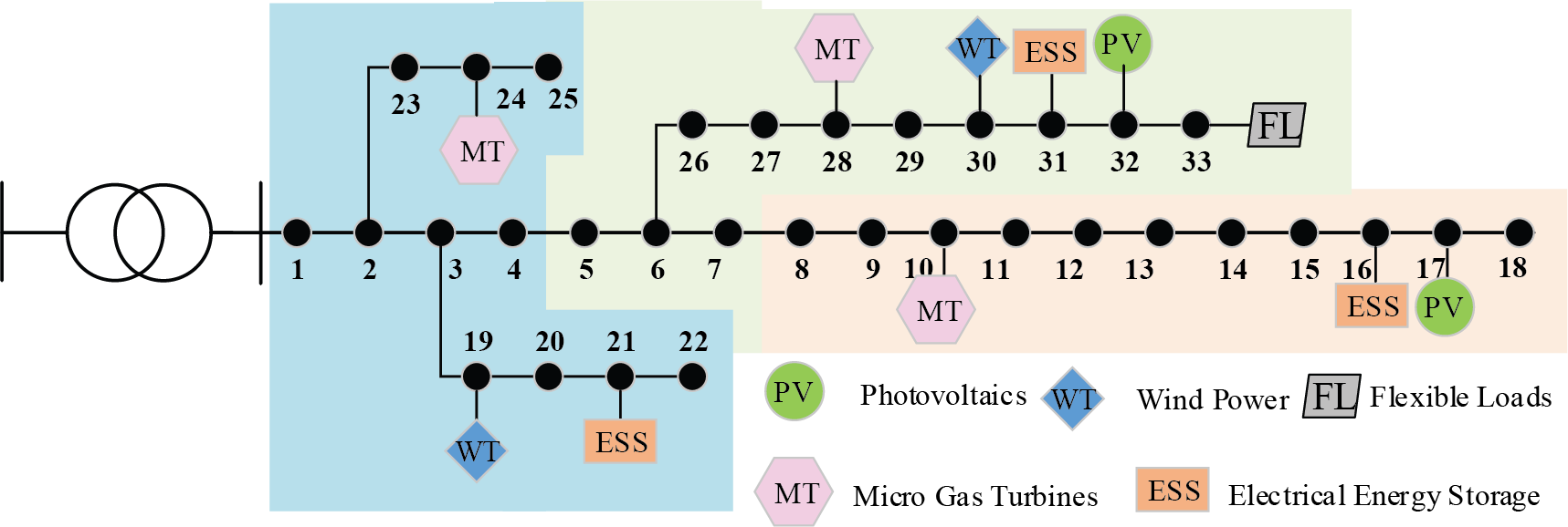
Figure 7: Network topology of the improved IEEE 33-node simulation system

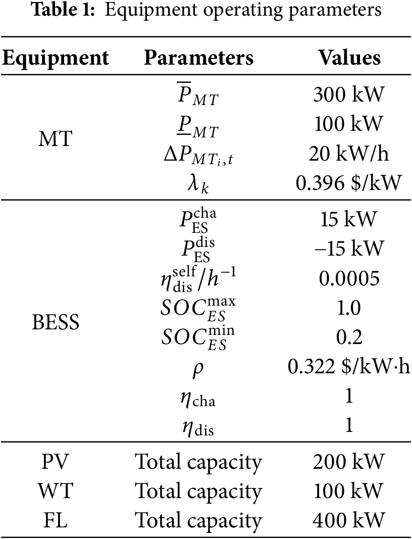
The test system was divided into three autonomous regions, as depicted in Fig. 6. The PV units, WT units, MTs, ESSs, and FLs were positioned at nodes {17, 32}, {19, 30}, {10, 24, 28}, {10, 24, 28}, and {33}, respectively. Fig. 8 illustrates the 24-h source-load forecast data and Table 1 provides the operational parameters of the equipment.

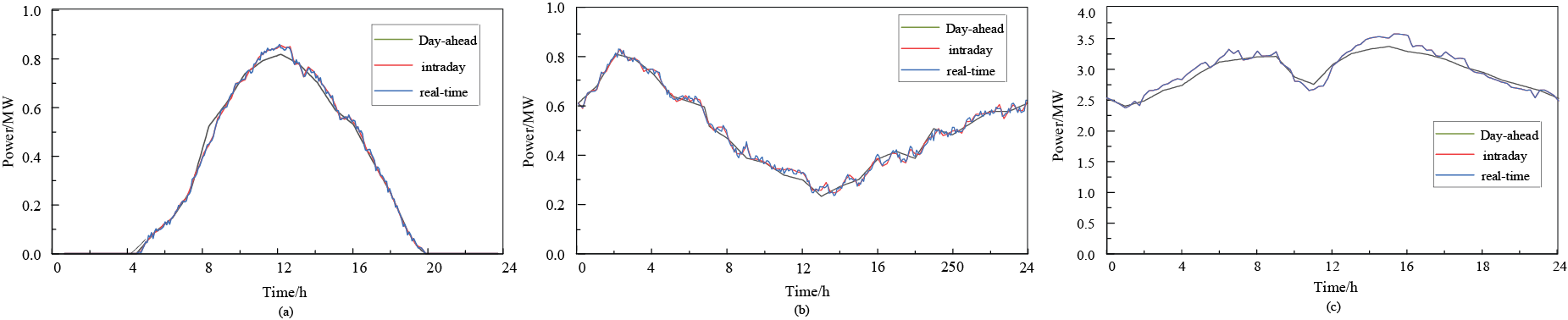
Figure 8: 24-h source-load forecasting data

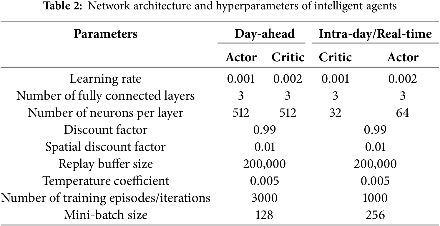
The performance of DRL algorithms is dependent on network architecture and hyperparameters. Network architecture influences the model’s representational capacity and policy approximation accuracy, while hyperparameters significantly influence the model’s learning efficiency and convergence behavior. Furthermore, key parameters like learning rate and discount factor play a crucial role in determining the algorithm’s outcome. Table 2 provides detailed configurations of network architecture and hyperparameters.

4.2 Comparison of Algorithm Convergence and Decision-Making Time

The SAC algorithm is a highly effective DRL method that efficiently balances the exploration-exploitation trade-off by maximizing both the expected reward and entropy of a policy, thus enhancing learning efficiency and performance. In this study, we introduced an improved adaptive temperature coefficient mechanism within the SAC framework, allowing dynamic temperature coefficient adjustments. This modification allows the algorithm to better accommodate environmental uncertainties and task-specific demands, leading to faster convergence and increased stability. We subsequently conducted a comparative analysis of the standard and modified SAC algorithms under identical environmental conditions and determined the rewards accumulated by the agent during the training process (Fig. 9).

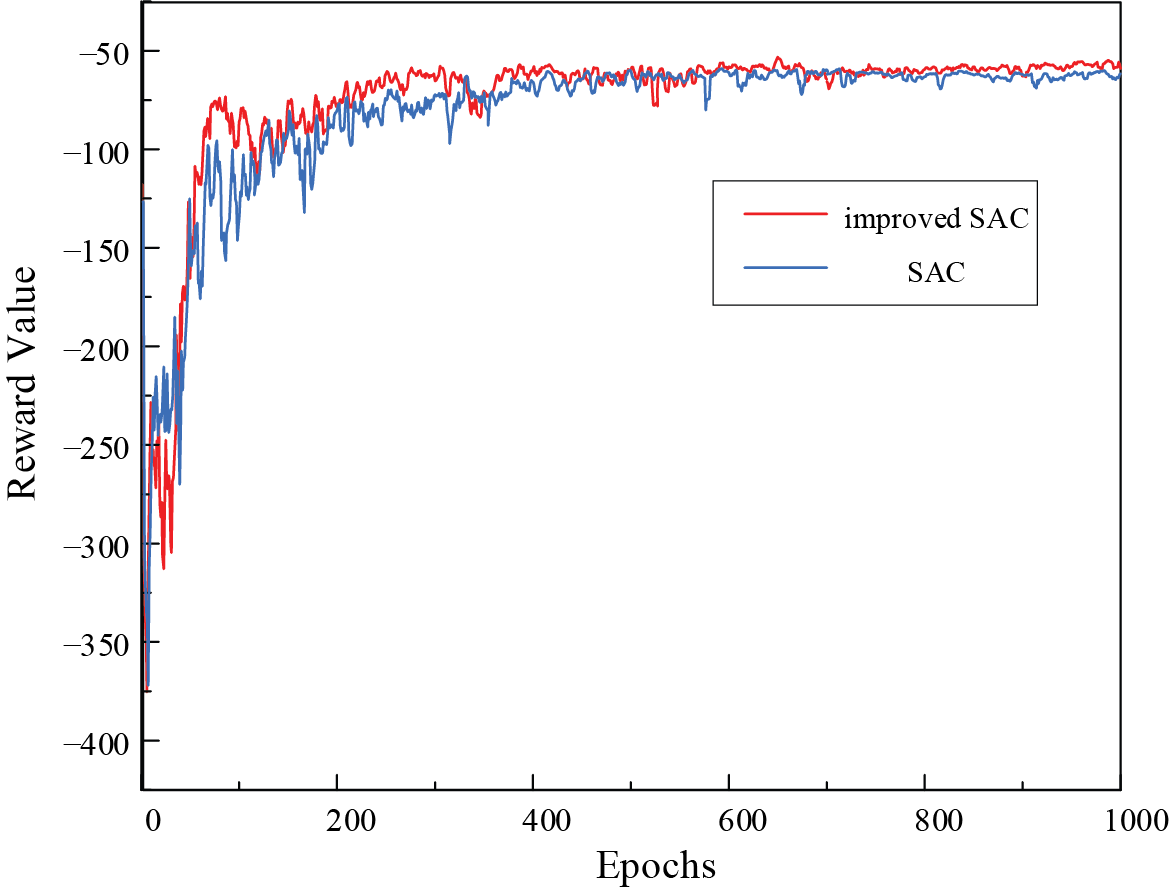
Figure 9: Convergence analysis of the SAC algorithm

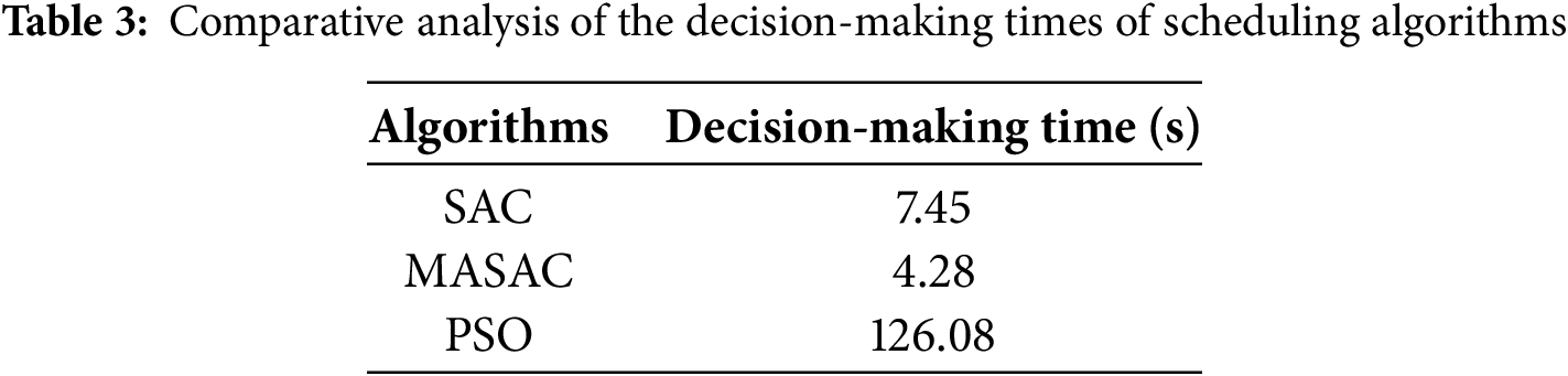
The agents were trained for a total of 1000 episodes. As illustrated in Fig. 4, the modified SAC algorithm achieved significantly high rewards within 100 episodes, while the standard SAC algorithm reached a similar performance level after approximately 400 episodes. These results demonstrate the superior convergence and learning speed of the modified SAC algorithm compared to the standard SAC algorithm. To further evaluate the decision-making speed of the MASAC algorithm, we integrated the SAC, MASAC, and Particle Swarm Optimization (PSO) algorithms into an intra-day optimization model. The results revealed that the MASAC algorithm exhibited a faster decision-making time than the SAC algorithm and significantly outperformed the PSO algorithm (Table 3).

4.3 Analysis of Scheduling Outcomes

(1)   Analysis of day-ahead scheduling outcomes

In the day-ahead stage, we optimized source-load-storage coordination based on the forecast data (Fig. 10), yielding optimal output schedules for various flexibility resources. In this study, we adopted a centralized scheduling approach for day-ahead dispatch.

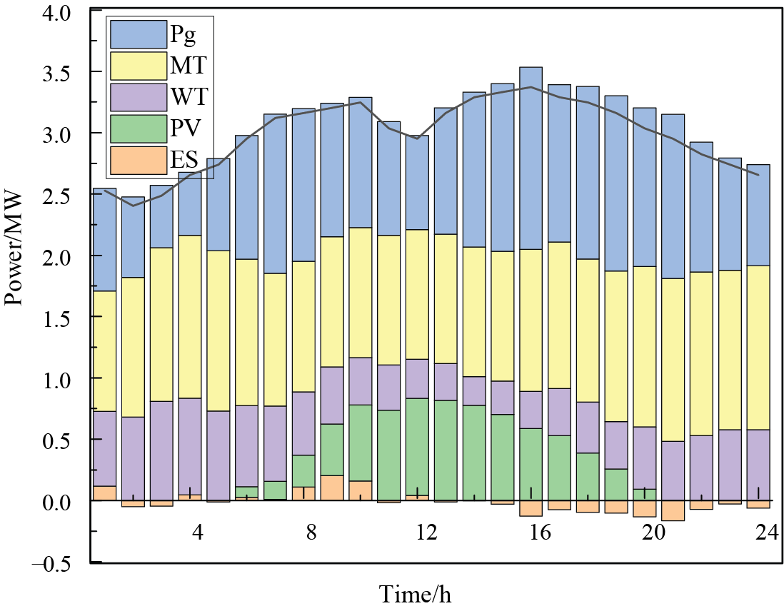
Figure 10: Graph of optimization results in the last 24 h

In the day-ahead scheduling model, full utilization of wind and solar resources was achieved through the coordinated optimization of source, load, and storage. The proactive interaction of flexible resources reduced the system’s overall operational costs during the intra-day stage. As seen in Fig. 11, the FLs that were originally scheduled between 13:00 and 18:00 were redistributed to 8:00 to 13:00 after optimization, achieving peak shaving and load leveling. As observed in Fig. 12, the output of MTs and ESSs across different regions showed minimal power fluctuations between 10:00 and 20:00, during the day-ahead stage. In Region A, the close proximity to the main bus and heightened sensitivity to electricity prices resulted in a reduction in power output between 2:00 and 4:00, followed by a subsequent increase from 4:00 to 6:00 (as illustrated in Fig. 12a). Conversely, in Region B, the significant share of distributed renewable energy contributed to a comparatively lower total output from MTs and ESSs (shown in Fig. 12b). This discrepancy can likely be explained by the inherent uncertainties tied to renewable energy generation, which may have impacted the overall system performance. However, both regions showed a rapid load increase from 4:00 to 6:00, leading to high load demands, necessitating increased output from the MTs and ESSs (Fig. 12). Subsequently, the total output decreased in response to increasing load uncertainty to preserve flexible capacity. ESS charging was predominantly influenced by electricity prices, especially before 5:00 and after 20:00.

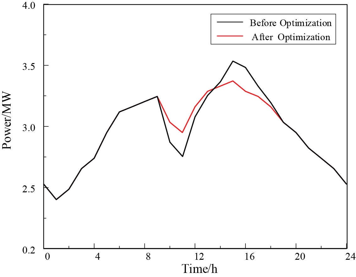
Figure 11: Comparative analysis of load data before and after optimization

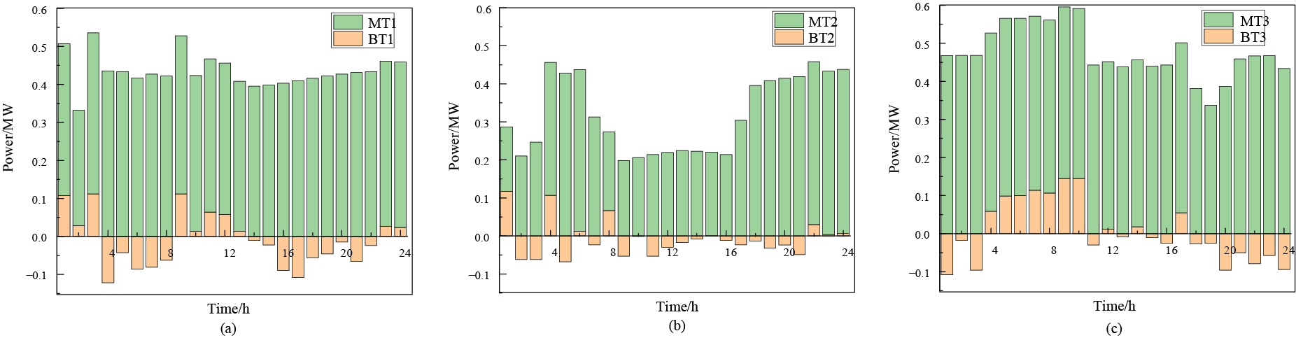
Figure 12: Output profiles of MTs and ESSs across different regions

Fig. 13 illustrates the daily flexibility supply and demand of the system. As illustrated in Fig. 13, the flexibility demand consistently exceeded the flexibility supply, with the demand increasing as it approaches the midpoint, followed closely by supply. This may be attributed to the Gaussian distribution of PV, WT, and FL forecast data. The central interval exhibited larger forecast fluctuations compared to the outer intervals. Additionally, since PV power generation was concentrated between 6:00 and 18:00, power fluctuations were more pronounced during this period.

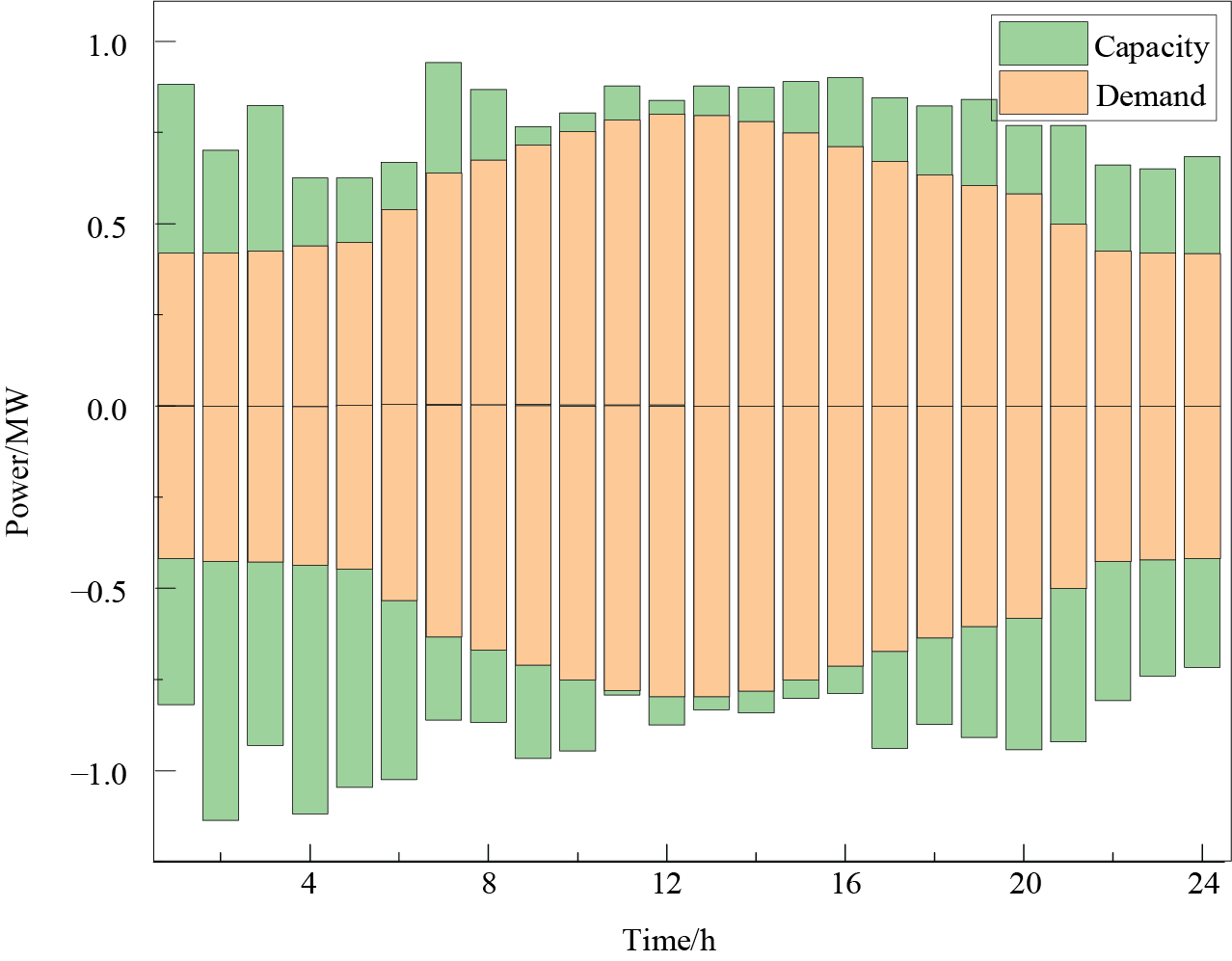
Figure 13: Comparative analysis of flexibility capacity and demand profiles

(2)   Analysis of intra-day scheduling outcomes

The intra-day optimization process builds upon the existing day-ahead scheduling strategy by adjusting the operational plans for MTs and ESSs. This ensures the balance between supply and demand within the grid while maximizing renewable energy utilization. Fig. 14 illustrates the variations in distributed MT output between day-ahead and intra-day operations across different regions, highlighting the significant impact of load fluctuations. The turbine output decreased between 9:00 to 13:00, corresponding with a notable decrease in load demand relative to the day-ahead predictions. Conversely, during other periods, the load demand exceeded the day-ahead forecasts, resulting in higher intra-day turbine output. Notably, Region 2, integrating both PV and WT, exhibited greater output volatility compared to the other regions.

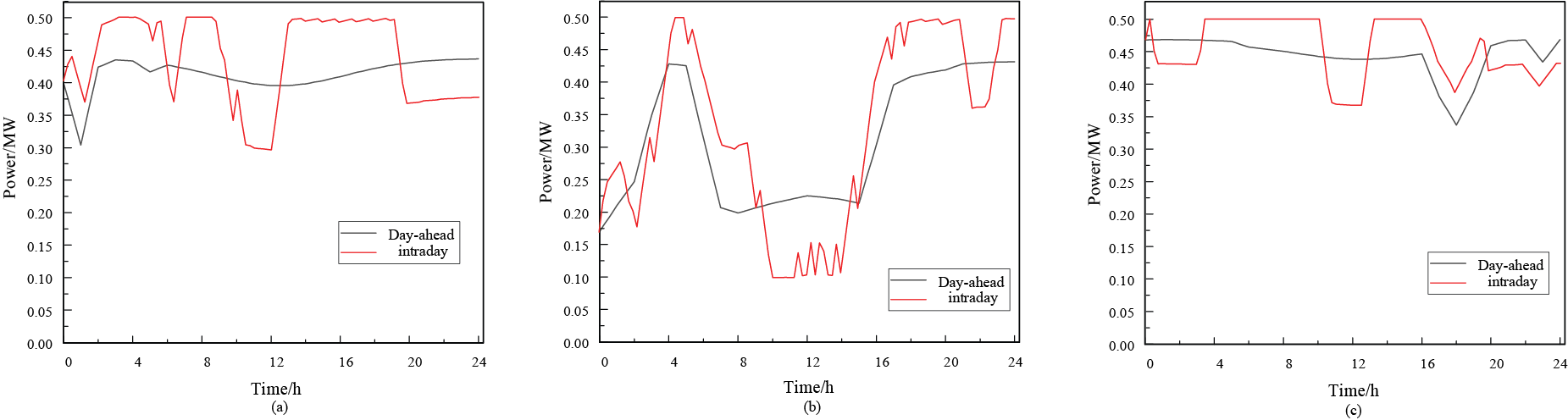
Figure 14: Convergence analysis of the algorithm

(3)   Analysis of real-time scheduling outcomes

The real-time correction phase involves rapid resource re-optimization, focusing primarily on distributed ESSs. Real-time scheduling optimization relies on intra-day rolling schedules to minimize adjustments and accommodate stochastic supply-demand fluctuations. Fig. 15 illustrates the regulation outcomes of the ESS, showing significant discrepancies between the real-time and day-ahead outcomes, which may be attributed to substantial variations between day-ahead and intra-day forecast data. The real-time phase focuses on mitigating the underutilization of renewable energy caused by supply-demand fluctuations by introducing minor but frequent adjustments to the ESS strategy.

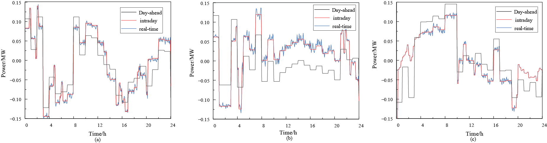
Figure 15: ESS scheduling strategy across multiple timescales

4.4 Scalability Experiments

To validate the scalability and adaptability of the proposed MASAC network model in larger DN systems, we constructed a 97-node DN system based on the original 33-node system through topology extension and parameter adjustment [33]. This expanded system retained the fundamental characteristics of the original system while tripling its scale, providing a more challenging test environment for evaluating algorithm performance. During the expansion process, we strictly adhered to the topological connection rules and electrical parameter constraints of the DNs to ensure that the expanded system has rational physical significance and engineering feasibility. Like the 33-node system, the expanded system utilized a partition management strategy and consisted of three interconnected regions, exhibiting similar operational parameters of distributed energy resources (including PV power, WT power, and MTs) and ESSs. This design ensured the comparability of experiments, providing an ideal experimental platform for studying the collaborative control capabilities of multi-agent systems in larger networks. The specific details of the 97-node DN system topology are illustrated in Fig. 16.

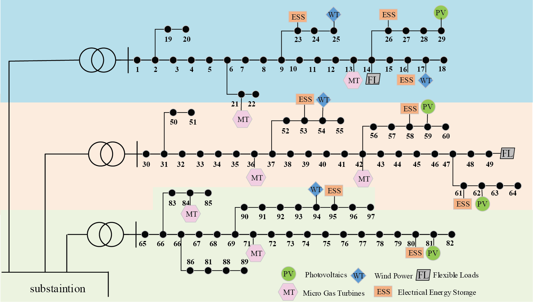
Figure 16: Schematic diagram of the 97-node DN system

(1)   Analysis of scheduling outcomes

A centralized optimization approach was employed to achieve optimal output schemes for various flexible resources through coordinated optimization of sources, loads, and storage, maximizing the utilization of wind and solar resources. Fig. 17a presents the data for each scheduling resource, and Fig. 17b illustrates the load operation status before and after regulation. The algorithm redistributes some of the FLs, originally concentrated between 13:00 and 18:00, to the 8:00 to 13:00 timeframe to achieve peak shaving and valley filling. As seen in Fig. 17c, the system’s flexibility supply and demand fluctuate throughout the day, with the supply consistently exceeding demand across all time periods. However, flexibility demand increased as it approached midday, aligning more closely with flexibility supply.

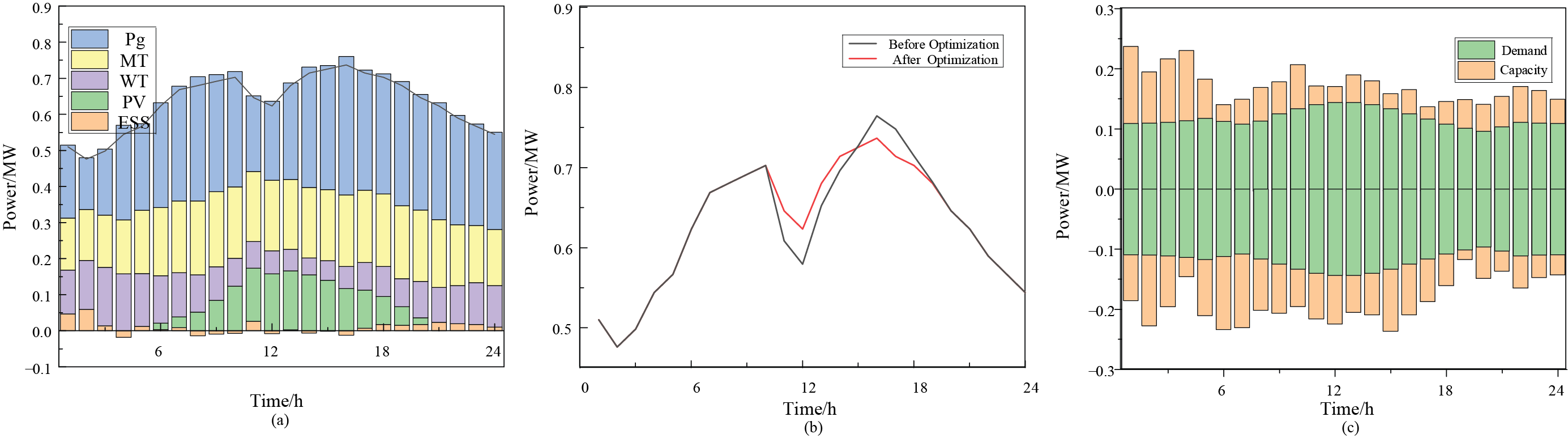
Figure 17: Day-ahead optimization outcomes

(2)   MT output performance

Fig. 18 illustrates the variations in the output of distributed MTs during day-ahead and intra-day dispatching. Fig. 18a and b, 18c and d, and 18e and f depicts the day-ahead scheduled output and intra-day actual output curves for MTs in Regions 1, 2, and 3, respectively. Based on the day-ahead scheduling outcomes, agents dynamically adjust MT output strategies in response to real-time load demands and fluctuations in WT and PV power generation, ensuring efficient utilization of distributed energy resources. Additionally, the algorithm demonstrates robust adaptability across regions of varying sizes. The results indicate that the proposed multi-agent optimization algorithm applies to both small- and large-scale DN systems, laying a foundation for its future application in more complex DN scenarios.

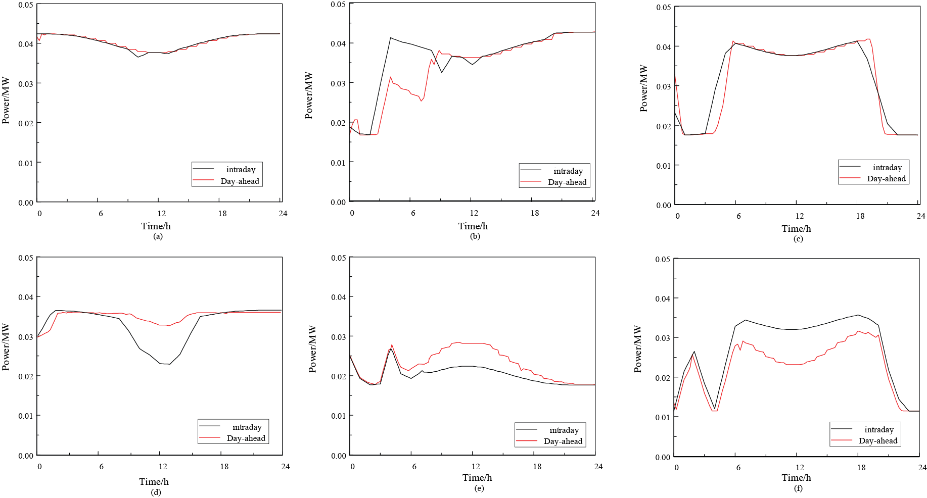
Figure 18: MT scheduling outcomes

(3)   Energy storage scheduling outcomes

Although real-time scheduling involves comparatively smaller adjustments, its higher regulation frequency allows for rapid responses to system fluctuations and efficient integration of renewable energy resources (Fig. 19). This regulatory characteristic was validated using the 97-node DN system, which demonstrated that the proposed multi-agent optimization algorithm possessed excellent scalability and adaptability. Our experimental results further demonstrate that the framework effectively regulates power DNs with high renewable energy integration. Altogether our study revealed that the MASAC model displays remarkable adaptability, robustness, and scalability in multi-agent environments, particularly in complex power distribution systems with an increasing number of nodes and distributed energy resources. These findings validate the model’s reliability and stability during scale expansion and provide theoretical support and practical feasibility for its application in large-scale ESSs.

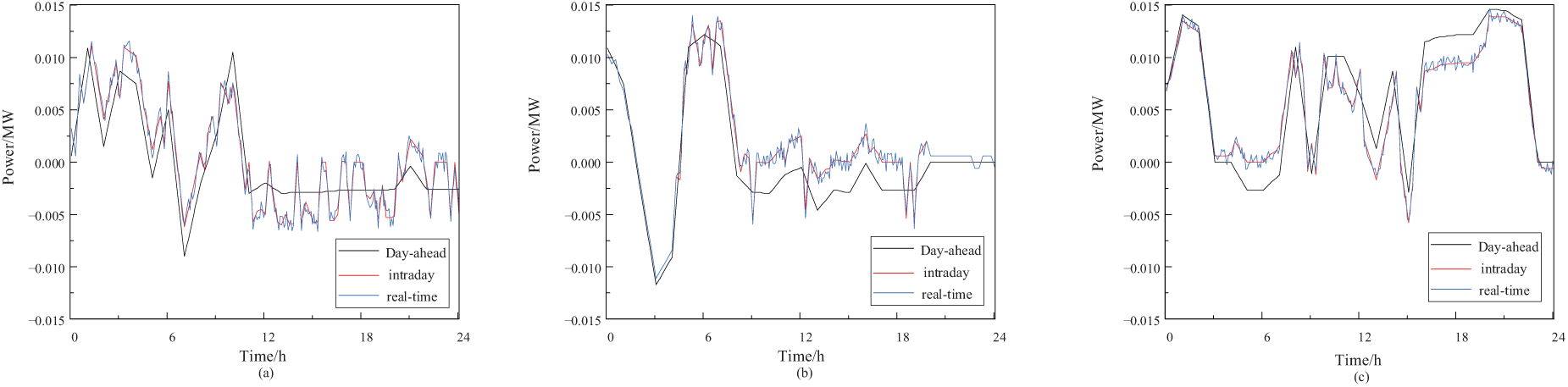
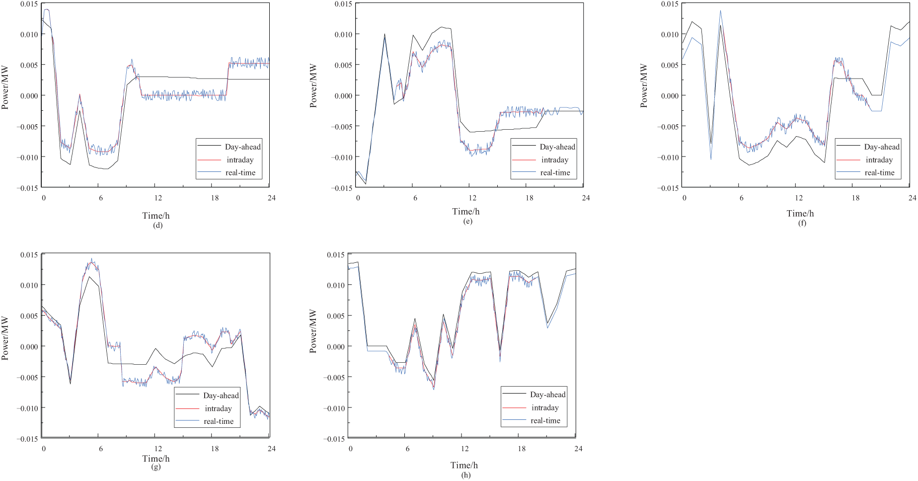
Figure 19: Comparison of multi-timescale ESS scheduling strategies

4.5 Additional Experiments

(1)   Robustness analysis

To comprehensively evaluate the robustness of the proposed multi-timescale optimization scheduling framework, we assessed its performance under varying day-ahead and intra-day source-load forecasting uncertainties. As shown in Tables 4 [34] and 5, this experiment employed identical base data to generate low, medium, and high uncertainty scenarios, with adjusted forecast fluctuation thresholds for WT and PV power generation and FL, corresponding to specific probabilistic distribution models. Our findings validate the effectiveness and reliability of the model for real-world applications.

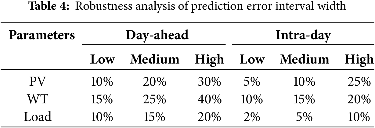
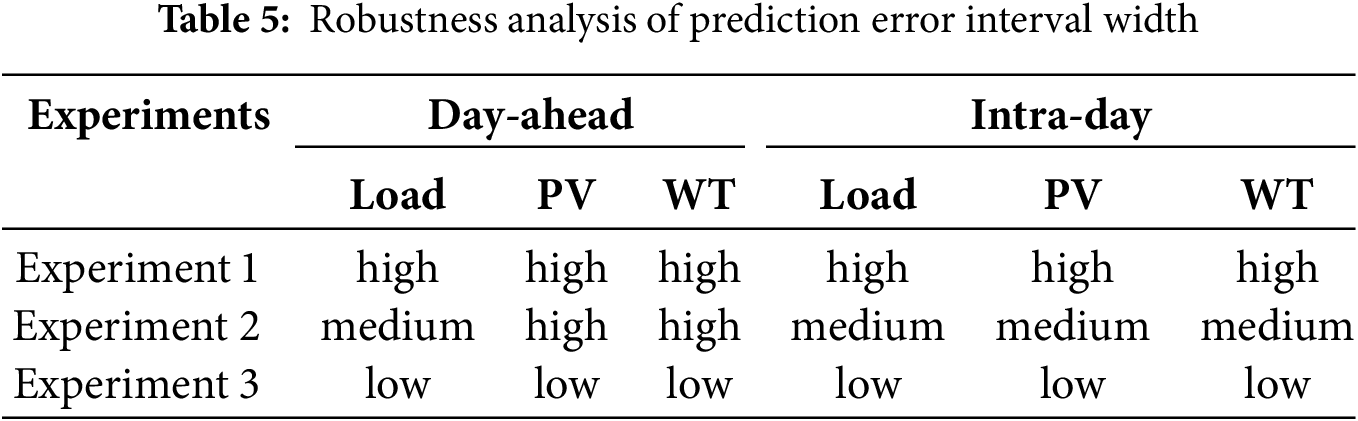
Table 6 provides an overview of dispatch costs, utilization rates, and capacity/demand ratios under various scenarios. These results reveal that the total system cost was significantly affected by day-ahead and intra-day purchase costs. The costs decreased significantly with a decrease in uncertainty. Specifically, the high uncertainty scenario incurred the highest costs, with total and day-ahead costs exceeding those of the moderate scenario by 3240.2 USD and 3664.8 USD, respectively. Meanwhile, the low uncertainty scenario offered further reductions of 1869.1 USD and 2427.1 USD in total and day-ahead costs, compared to the moderate scenario.

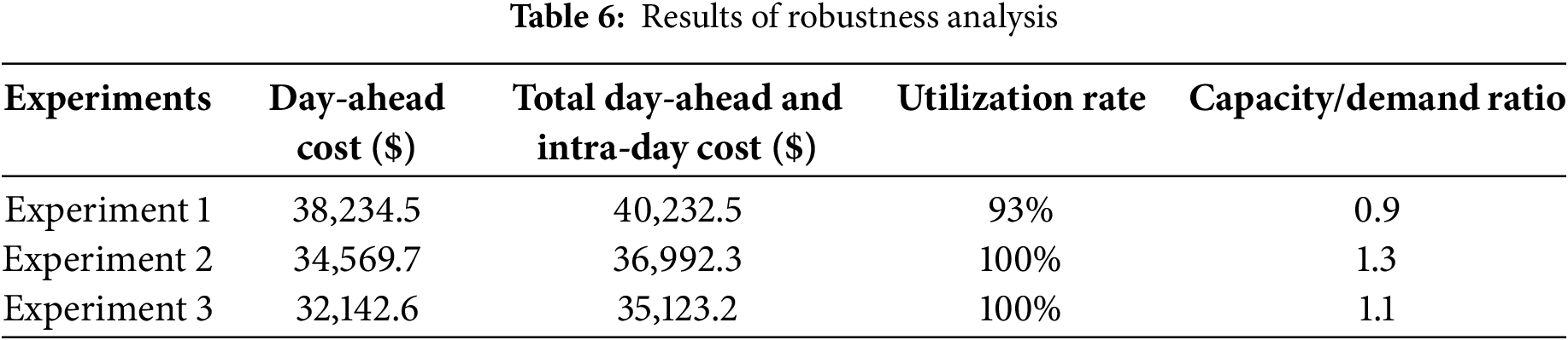
The high uncertainty scenario faced various challenges, such as increased external electricity purchases and scheduling difficulties, which were attributed to insufficient flexibility of ESSs and MTs. This was reflected in a lower capacity/demand ratio of 0.9, indicating underutilization of resources. In contrast, the moderate uncertainty scenario achieved a 100% resource utilization rate and a 1.3 capacity/demand ratio, suggesting a more balanced allocation of resources, resulting in significant cost savings and stability. Lastly, the low uncertainty scenario showed further optimization of resource utilization and efficiency. However, as low uncertainty conditions are less common in real-world settings, the moderate uncertainty strategy was deemed to be more practical and robust for real-world applications. In conclusion, the proposed multi-timescale optimization dispatch framework exhibited robust performance across varying levels of uncertainty. While high uncertainty scenarios pose cost and flexibility challenges, moderate uncertainty scenarios effectively maintain cost, resource utilization, and system stability, demonstrating high adaptability and efficiency of the framework in managing source-load forecast uncertainties.

(2)   Comparison of results

Considering the source-load uncertainty range, the proposed method can better calculate the flexibility demand capacity, ensuring a stable power supply. To more effectively evaluate the significance of the proposed method, three sets of multi-time-scale scheduling methods are used as control groups: Method 1 disregards the source-load uncertainty range and uses deterministic optimization; Method 2 employs robust optimization to account for the worst-case scenario in the day-ahead optimization, while intra-day and real-time adjustments are made using a rolling optimization approach [34]. Method 3 utilizes the Copula function in the day-ahead stage to generate scenarios that describe the uncertainty in source-load prediction data, with intra-day and real-time rolling adjustments [35]. Method 4 is the method proposed in this paper. During the comparison, we calculated the grid cost, renewable energy absorption, and flexibility capacity for each method, as shown in Table 7.

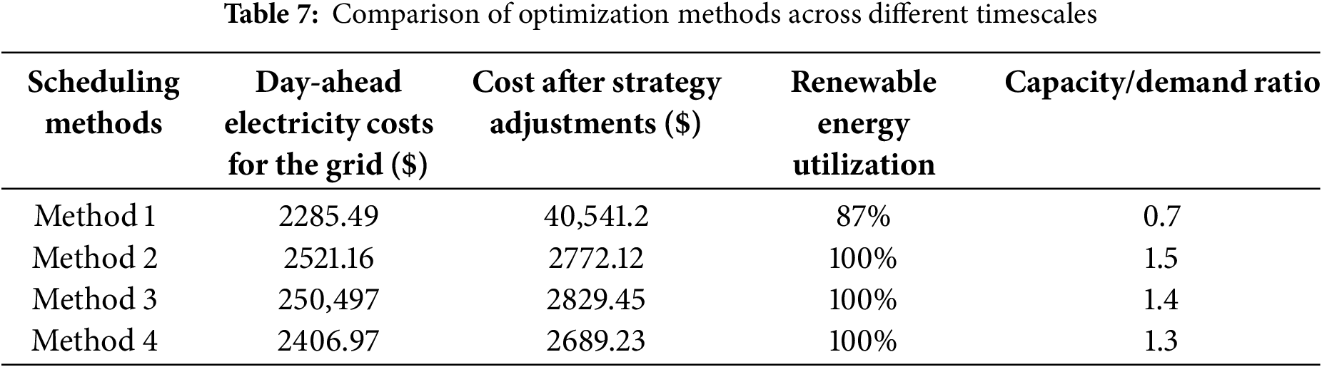
The results show that Method 4 (that is, the method in this paper) has the best performance on the day and day combined cost. Compared with Method 1, which has the highest cost, the cost is reduced by $364.89, or about 11.95%; In terms of the combined cost of daily grid electricity, Method 4 led the way at $2406.97, a decrease of $114.19 (4.53%) compared to Method 2 and $98 (3.91%) compared to Method 3. In terms of the absorption of new energy, Methods 2, 3, and 4 all achieve a 100% absorption rate, while Method 1 is only 87%, which shows that the method in this paper is more effective in using renewable energy. Especially in terms of capacity requirements, Method 4 requires a smaller flexible demand capacity (1.3), 13.3% lower than Method 2, while maintaining power system stability. Overall, the experimental results prove that the proposed method can effectively reduce the comprehensive cost by about 12% under medium uncertainty conditions, increase the energy absorption rate to 100%, and ensure a stable power supply with a low flexible capacity of 1.3, showing significant application potential and practical value in multi-timescale scheduling.

5  Conclusions and Future Perspectives

This study proposes a multi-timescale DN optimization scheduling method that considers uncertainty intervals, which is solved using an improved Soft Actor-Critic algorithm and a Multi-Agent SAC algorithm. This approach effectively addresses the challenges posed by source-load prediction uncertainties. The main contributions are as follows:

(1)   Uncertainty Interval Optimization Method: By integrating uncertainty intervals of source-load predictions, this method resolves the flexibility requirements and capacity constraints in power grid scheduling, significantly enhancing the system’s economic efficiency and renewable energy accommodation capability.

(2)   Improved SAC Algorithm: Through adaptive adjustment of the temperature coefficient, the exploration capability of the agent is enhanced, making the training process more stable while reducing policy fluctuations.

(3)   Multi-Agent Real-Time Optimization: The multi-agent model based on the CTDE framework significantly reduces the computation time for intra-day and real-time strategy generation, ensuring the real-time performance of scheduling strategies.

When applying the methodology presented in this paper to the optimization scheduling of real-world DNs, we encounter a range of complex challenges. Firstly, the training of agents is highly dependent on a substantial amount of authentic DN simulation data, which is often difficult to obtain due to confidentiality and security requirements. Although our improved SAC algorithm partially mitigates the dependency on a fixed DN framework, the need for high-quality training data remains a critical issue. To address these challenges, future advancements must focus on the development of innovative data generation and simulation techniques, as well as enhancing the algorithm’s adaptability under incomplete data conditions. Furthermore, interdisciplinary collaboration and the development of new technological tools will play a crucial role in facilitating the practical application of these techniques within DN systems. These efforts will ultimately contribute to improving the operational efficiency of power distribution systems and accelerating the integration and application of renewable energy sources.

Acknowledgement: Not applicable.

Funding Statement: This research was funded by Jilin Province Science and Technology Development Plan Project, grant number 20220203163SF.

Author Contributions: The authors confirm their contribution to the paper as follows: study conception and design: Huanan Yu, Shiqiang Li; data collection: Jinling Li, Jing Bian; analysis and interpretation of results: Chunhe Ye, Shiqiang Li, He Wang, Huanan Yu; draft manuscript preparation: Chunhe Ye, Shiqiang Li, Huanan Yu. All authors reviewed the results and approved the final version of the manuscript.

Availability of Data and Materials: The authors confirm that the data supporting the findings of this study are available within the article. And the additional data that support the findings of this study are available on request from the corresponding author, upon reasonable request.

Ethics Approval: This study did not involve any human or animal subjects.

Conflicts of Interest: The authors declare no conflicts of interest to report regarding the present study.

Abbreviations

References

1. Singh S, Singh S. Advancements and challenges in integrating renewable energy sources into distribution grid systems: a comprehensive review. J Energy Resour Technol. 2024;146(9):090801. doi:10.1115/1.4065503. [Google Scholar] [CrossRef]

2. Tao Y, Qiu J, Lai S, Zhao J, Xue Y. Carbon-oriented electricity network planning and transformation. IEEE Trans Power Syst. 2021;36(2):1034–48. doi:10.1109/TPWRS.2020.3016668. [Google Scholar] [CrossRef]

3. Fang Y, Han J, Du E, Jiang H, Fang Y, Zhang N, et al. Electric energy system planning considering chronological renewable generation variability and uncertainty. Appl Energy. 2024;373(2):123961. doi:10.1016/j.apenergy.2024.123961. [Google Scholar] [CrossRef]

4. Gbadega PA, Sun YX. JAYA algorithm-based energy management for a grid-connected micro-grid with PV-wind-microturbine-storage energy system. Int J Eng Res Afr. 2023;63(1):159–84. doi:10.4028/p-du1983. [Google Scholar] [CrossRef]

5. Su J, Anokhin D, Dehghanian P, Lejeune MA. On the use of mobile power sources in distribution networks under endogenous uncertainty. IEEE Trans Control Netw Syst. 2023;10(4):1937–49. doi:10.1109/TCNS.2023.3256278. [Google Scholar] [CrossRef]

6. Chowdhury MMUT, Biswas BD, Kamalasadan S. Second-order cone programming (SOCP) model for three phase optimal power flow (OPF) in active distribution networks. IEEE Trans Smart Grid. 2023;14(5):3732–43. doi:10.1109/TSG.2023.3241216. [Google Scholar] [CrossRef]

7. Kiani S, Sheshyekani K, Dagdougui H. ADMM-based hierarchical single-loop framework for EV charging scheduling considering power flow constraints. IEEE Trans Transp Electrif. 2023;10(1):1089–1100. doi:10.1109/TTE.2023.3269050. [Google Scholar] [CrossRef]

8. Li S, Bao G, Zhang A. Consensus-based distributed coordinated operation of active distribution networks with electric heating loads. Int J Electr Power Energy Syst. 2023;153(4):109393. doi:10.1016/j.ijepes.2023.109393. [Google Scholar] [CrossRef]

9. Ruan H, Gao H, Liu Y, Wang L, Liu J. Distributed voltage control in active distribution network considering renewable energy: a novel network partitioning method. IEEE Trans Power Syst. 2020;35(6):4220–31. doi:10.1109/TPWRS.2020.3000984. [Google Scholar] [CrossRef]

10. Wu Z, Li Y, Gu W, Dong Z, Zhao J, Liu W, et al. Multi-timescale voltage control for distribution system based on multi-agent deep reinforcement learning. Int J Electr Power Energy Syst. 2023;147(7):108830. doi:10.1016/j.ijepes.2022.108830. [Google Scholar] [CrossRef]

11. Dong G, Chen Z. Data-driven energy management in a home microgrid based on Bayesian optimal algorithm. IEEE Trans Ind Inform. 2018;15(2):869–77. doi:10.1109/TII.2018.2820421. [Google Scholar] [CrossRef]

12. Park K, Moon I. Multi-agent deep reinforcement learning approach for EV charging scheduling in a smart grid. Appl Energy. 2022;328(1):120111. doi:10.1016/j.apenergy.2022.120111. [Google Scholar] [CrossRef]

13. Wang G, Sun Y, Li J, Jiang Y, Li C, Yu H, et al. Dynamic economic scheduling with self-adaptive uncertainty in distribution network based on deep reinforcement learning. Energy Eng. 2024;121(6):1671–95. doi:10.32604/ee.2024.047794. [Google Scholar] [CrossRef]

14. Li P, Wei M, Ji H, Xi W, Yu H, Wu J, et al. Deep reinforcement learning-based adaptive voltage control of active distribution networks with multi-terminal soft open point. Int J Electr Power Energy Syst. 2022;141(2):108138. doi:10.1016/j.ijepes.2022.108138. [Google Scholar] [CrossRef]

15. Lyu X, Baisero A, Hao Y, Daley B, Amato C. On centralized critics in multi-agent reinforcement learning. J Artif Intell Res. 2023;77:295–354. doi:10.1613/jair.1.14386. [Google Scholar] [CrossRef]

16. Li L, Wang J, Li W, Peng Q, Chen X, Li S. Decentralized decision for multi-band sensing: a deep reinforcement learning approach. IEEE Wirel Commun Lett. 2021;10(12):2674–7. doi:10.1109/LWC.2021.3111750. [Google Scholar] [CrossRef]

17. Cao D, Zhao J, Hu W, Yu N, Ding F, Huang Q, et al. Deep reinforcement learning enabled physical-model-free two-timescale voltage control method for active distribution systems. IEEE Trans Smart Grid. 2022;13(1):149–65. doi:10.1109/TSG.2021.3113085. [Google Scholar] [CrossRef]

18. Rayati M, Bozorg M, Carpita M, Cherkaoui R. Stochastic optimization and Markov chain-based scenario generation for exploiting the underlying flexibilities of an active distribution network. Sustainable Energy Grids Networks. 2023;34(2):100999. doi:10.1016/j.segan.2023.100999. [Google Scholar] [CrossRef]

19. Al-Lawati RA, Faiz TI, Noor-E-Alam M. A nationwide multi-location multi-resource stochastic programming based energy planning framework. Energy. 2024;295:130898. doi:10.1016/j.energy.2024.130898. [Google Scholar] [CrossRef]

20. Mohseni S, Pishvaee MS. Energy trading and scheduling in networked microgrids using fuzzy bargaining game theory and distributionally robust optimization. Appl Energy. 2023;350:121748. doi:10.1016/j.apenergy.2023.121748. [Google Scholar] [CrossRef]

21. Nammouchi A, Aupke P, D’Andreagiovanni F, Ghazzai H, Theocharis A, Kassler A. Robust opportunistic optimal energy management of a mixed microgrid under asymmetrical uncertainties. Sustainable Energy Grids Networks. 2023;36(4):101184. doi:10.1016/j.segan.2023.101184. [Google Scholar] [CrossRef]

22. Li C, Li Y, Peng S, Wang P, Ge Q, Song L, et al. A two-stage adaptive-robust optimization model for active distribution network with high penetration wind power generation. IET Renew Power Gener. 2024;18(7):1204–17. doi:10.1049/rpg2.12836. [Google Scholar] [CrossRef]

23. Esteban-Pérez A, Morales JM. Distributionally robust optimal power flow with contextual information. Eur J Oper Res. 2023;306(3):1047–58. doi:10.1016/j.ejor.2022.10.024. [Google Scholar] [CrossRef]

24. Jiang C, Zhang QF, Han X, Li D, Liu J. An interval optimization method considering the dependence between uncertain parameters. Comp Model Eng Sci. 2011;74(1):65–82. doi:10.3970/cmes.2011.074.065. [Google Scholar] [CrossRef]

25. Xu H, Chang Y, Zhao Y, Wang F. A new multi-timescale optimal scheduling model considering wind power uncertainty and demand response. Int J Electr Power Energy Syst. 2023;147(2):108832. doi:10.1016/j.ijepes.2022.108832. [Google Scholar] [CrossRef]

26. Li Q, Zhao N. A probability box representation method for power flow analysis considering both interval and probabilistic uncertainties. Int J Electr Power Energy Syst. 2022;142(1):108371. doi:10.1016/j.ijepes.2022.108371. [Google Scholar] [CrossRef]

27. Tan Q, Mei S, Dai M, Zhou L, Wei Y, Ju L. A multi-objective optimization dispatching and adaptability analysis model for wind-PV-thermal-coordinated operations considering comprehensive forecasting error distribution. J Clean Prod. 2020;256(3):120407. doi:10.1016/j.jclepro.2020.120407. [Google Scholar] [CrossRef]

28. Wang MQ, Gooi HB. Spinning reserve estimation in microgrids. IEEE Trans Power Syst. 2011;26(3):1164–74. doi:10.1109/TPWRS.2010.2100414. [Google Scholar] [CrossRef]

29. Jin J, Xu Y. Optimal policy characterization enhanced actor-critic approach for electric vehicle charging scheduling in a power distribution network. IEEE Trans Smart Grid. 2020;12(2):1416–28. doi:10.1109/TSG.2020.3028470. [Google Scholar] [CrossRef]

30. Zhao Z, Zhang Y, Wang S, Zhang F, Zhang M, Chen W. QDAP: downsizing adaptive policy for cooperative multi-agent reinforcement learning. Knowl Based Syst. 2024;294(1):111719. doi:10.1016/j.knosys.2024.111719. [Google Scholar] [CrossRef]

31. Deng L, Huan J, Wang W, Zhang W, Xie L, Dong L, et al. Market operation of energy storage system in smart grid: a review. Energy Eng. 2024;121(6):1403–37. doi:10.32604/ee.2024.046393. [Google Scholar] [CrossRef]

32. Qiu S, Deng Y, Ding M, Han W. An optimal scheduling method for distribution network clusters considering source-load–storage synergy. Sustainability. 2024;16(15):6399. doi:10.3390/su16156399. [Google Scholar] [CrossRef]

33. Lu Y, Xiang Y, Huang Y, Yu B, Weng L, Liu J. Deep reinforcement learning based optimal scheduling of active distribution system considering distributed generation, energy storage and flexible load. Energy. 2023;271(4):127087. doi:10.1016/j.energy.2023.127087. [Google Scholar] [CrossRef]

34. Hou J, Yu W, Xu Z, Ge Q, Li Z, Meng Y. Multi-time scale optimization scheduling of microgrid considering source and load uncertainty. Elect Power Syst Res. 2023;216(32):109037. doi:10.1016/j.epsr.2022.109037. [Google Scholar] [CrossRef]

35. Shan X, Xue F. A day-ahead economic dispatch scheme for transmission system with high penetration of renewable energy. IEEE Access. 2022;10(12):11159–72. doi:10.1109/ACCESS.2022.3145973. [Google Scholar] [CrossRef]