Distributed Photovoltaic Power Prediction Technology Based on Spatio-Temporal Graph Neural Networks

1  Introduction

Renewable energy is considered a viable alternative to fossil fuels, offering a means to mitigate their adverse environmental impacts [1]. Photovoltaic (PV) power generation technology converts solar energy into electricity, providing a sustainable and clean energy source. Its adoption has grown rapidly in recent years. Solar resources are abundant, widely distributed, and easily accessible, with their development accelerated by favorable policies [2]. By the end of June 2024, China’s total installed PV capacity had reached 713 GW, a 52% year-on-year increase, comprising 403 GW from centralized PV systems and 310 GW from distributed PV systems [3].

Despite rapid advancements and expanding applications of PV technology, several challenges remain. PV power output is inherently dependent on solar irradiance, which is affected by weather conditions and diurnal cycles, resulting in considerable output uncertainty [4]. This intermittency and volatility can disrupt grid stability by challenging the real-time balance among generation, transmission, and consumption. Therefore, accurate PV power forecasting is critical. Forecasting aims to predict future power output using historical data and relevant variables. Reliable forecasts enable grid operators to optimize generation planning, ensure stable operation, and support intelligent energy management [5].

PV forecasting methods are generally categorized into three types: statistical methods, machine learning techniques, and deep learning approaches. Statistical methods include autoregressive analysis [6,7], exponential smoothing [8,9], Kalman filtering [10,11], multivariate linear regression [12,13], and autoregressive integrated moving average models [14,15]. These techniques typically leverage historical data to capture temporal correlations with low computational cost. However, their performance is often limited by their inability to model nonlinear dynamics effectively. Machine learning methods, such as neural networks and support vector machines (SVM), improve upon traditional methods by capturing complex nonlinear relationships in operational data, thereby enhancing prediction accuracy and generalizability.

Spatio-temporal modeling techniques have recently emerged to jointly capture temporal dependencies and spatial correlations among geographically distributed PV sites. Approaches such as graph neural networks and spatial autoregression [16,17] enhance prediction by transforming spatially related features into enriched inputs. Notable examples include the Graph Multi-Attention Network (GMAN) proposed by Zheng et al. [18], which uses transformed attention layers for feature extraction and error mitigation; the Temporal Polynomial Graph Neural Network (TPGNN) by Liu et al. [19], which applies temporal matrix polynomials to model multivariate time-series correlations; and the dynamic graph construction method of Han et al. [20], which integrates temporal data into static adjacency matrices for road network modeling. However, these methods are sensitive to outliers and often require large-scale historical datasets. Recent deep learning developments have improved prediction accuracy by modeling nonlinear interactions [21,22]. CNN-based models have been used to extract features between PV output and environmental factors, often combined with SVM for prediction, though they may overlook the inherent volatility of renewable energy [23]. While Recurrent Neural Networks (RNNs) perform well in short-term forecasting, they often underexploit temporal structures in PV sequences [24]. Hybrid models, such as those combining K-means clustering with LSTM networks, address environmental coupling but are limited in scope [25]. Although RNN-based sequence models (e.g., LSTM, GRU, attention-enhanced LSTM) demonstrate strong temporal modeling capabilities [26–28], they suffer from limitations such as gradient vanishing/exploding in long sequences [29,30] and tend to underexplore spatial features [31]. In PV-dense regions with abundant solar resources [32,33], insufficient mining of spatial correlations has limited predictive performance.

Moreover, most existing models are trained and deployed locally, making them better suited for centralized PV systems. Centralized PV requires large land areas, expensive infrastructure, and complex maintenance, while distributed PV—installed near end-users—offers more flexible and efficient local energy utilization [34,35]. The DEST-GNN model addresses the spatiotemporal correlation characteristics of distributed photovoltaic (PV) power stations by integrating Graph Convolutional Network (GCN) and Temporal Convolutional Network (TCN) modules to jointly model spatial and temporal dependencies, thereby improving the prediction accuracy of distributed PV power generation. However, the current implementation only evaluates the model’s predictive performance at a minimum temporal resolution of 30 min, failing to explore its potential in real-time application scenarios [36]. However, distributed PV systems face additional challenges in forecasting due to data quality and model transferability. Prediction models trained for specific locations often fail under different environmental or operational conditions. Thus, it is crucial to develop accurate and robust models tailored to the characteristics of distributed PV datasets to support broader applicability and integration into the power grid.

In this study, we propose a distributed PV power forecasting model based on a Spatio–Temporal Graph Neural Network (STGNN). In this model, each PV plant is represented as a node in an undirected graph, with edges denoting output correlations between nodes. A sparse attention mechanism is introduced to filter out weak temporal and spatial dependencies, enabling the model to focus on significant correlations and improve the prediction accuracy for distributed PV systems.

2  Spatio-Temporal Graph Neural Network Prediction Model Construction

2.1 Graph Convolutional Network for PV Prediction

GCN is a deep learning-based framework that facilitates feature extraction and representation learning directly on graph-structured data [37,38]. Its core idea is to capture local structural information and feature dependencies between nodes in a graph by defining convolutional operations on the graph. A graph can be defined as:

V={M,E}(1)

where M denotes the subset of nodes of the graph and denotes the subset of edges of the graph. Based on edge directionality, graphs can be classified into directed and undirected graphs. In a directed graph, edges are directional and typically represented as ordered pairs (mi, mj), indicating a connection from node mi to node mj. In contrast, in an undirected graph, edges are bidirectional and represented as unordered pairs (mi, mj), indicating a symmetric connection between nodes mi and mj. Therefore, if all edges in a graph are bidirectionally connected (e.g., (mi,mj)∈E), the graph is classified as an undirected graph.

For a specific graph structure, its corresponding vector space embedding can be constructed to map the graph data into a low-dimensional continuous vector space. The normalized graph Laplacian matrix L∈RM×M can be expressed as:

L=IM−D−12AD12(2)

where is the unit matrix, A∈RM×M is the adjacency matrix, ai,j=1 when there is an edge between nodes mi and mj otherwise ai,j=0. It can be expressed as:

A={ai,j=1,(mi,mj)∈Eai,j=0, otherwise(3)

The degree matrixs D∈RM×M is a diagonal matrix and L∈RM×M can be expressed as:

D={di,j=∑j=1Mai,j,diagonaldi,j=0,otherwise(4)

The core objective of Convolutional Graph Neural Networks (ConvGNNs) is to perform feature extraction and representation learning on graph-structured data by mapping input features to high-level representations. This is achieved by aggregating information from neighboring nodes through graph convolution operations. The process can be formulated as:

x(t)^=x(t)∗Gk(5)

where x(t) denotes the input feature vector, ∗G represents the graph convolution transportation, k denotes the kernel of the system, and x(t)^ is the transformed output. By feature decomposition and simplification, and based on the graph Laplacian matrix L defined in Eqs. (2) and (4), the graph convolution transportation can be further represented as:

x(t)∗Gk=θLx(t)(6)

where θ denotes the manageable parameters of the model, and L represents the graph Laplacian matrix calculated according to the above definition.

Unlike traditional CNNs that operate on regular grid-like data (e.g., images), GCNs are capable of processing graph-structured data with arbitrary topologies, such as social networks, molecular structures, and knowledge graphs. By utilizing both the structural information and node features of the graph, GCNs learn expressive node representations through iterative neighborhood aggregation. This enables them to support downstream tasks such as node classification, graph classification, and link prediction.

For PV power prediction, each PV module within a power plant can be represented as a node, with connections between modules modeled as edges. The spatial correlations among neighboring modules can be effectively captured by GCN convolution operations, thereby improving the accuracy of PV power forecasting [39].

2.2 STGNN Architecture and Approach

The methodology proposed in this paper introduces a novel model, STGNN, for intra-hour PV power forecasting across multiple sites. This approach is specifically designed to effectively capture the complex spatio-temporal correlations among PV stations, thereby improving forecasting accuracy. The overall model structure is illustrated in Fig. 1.

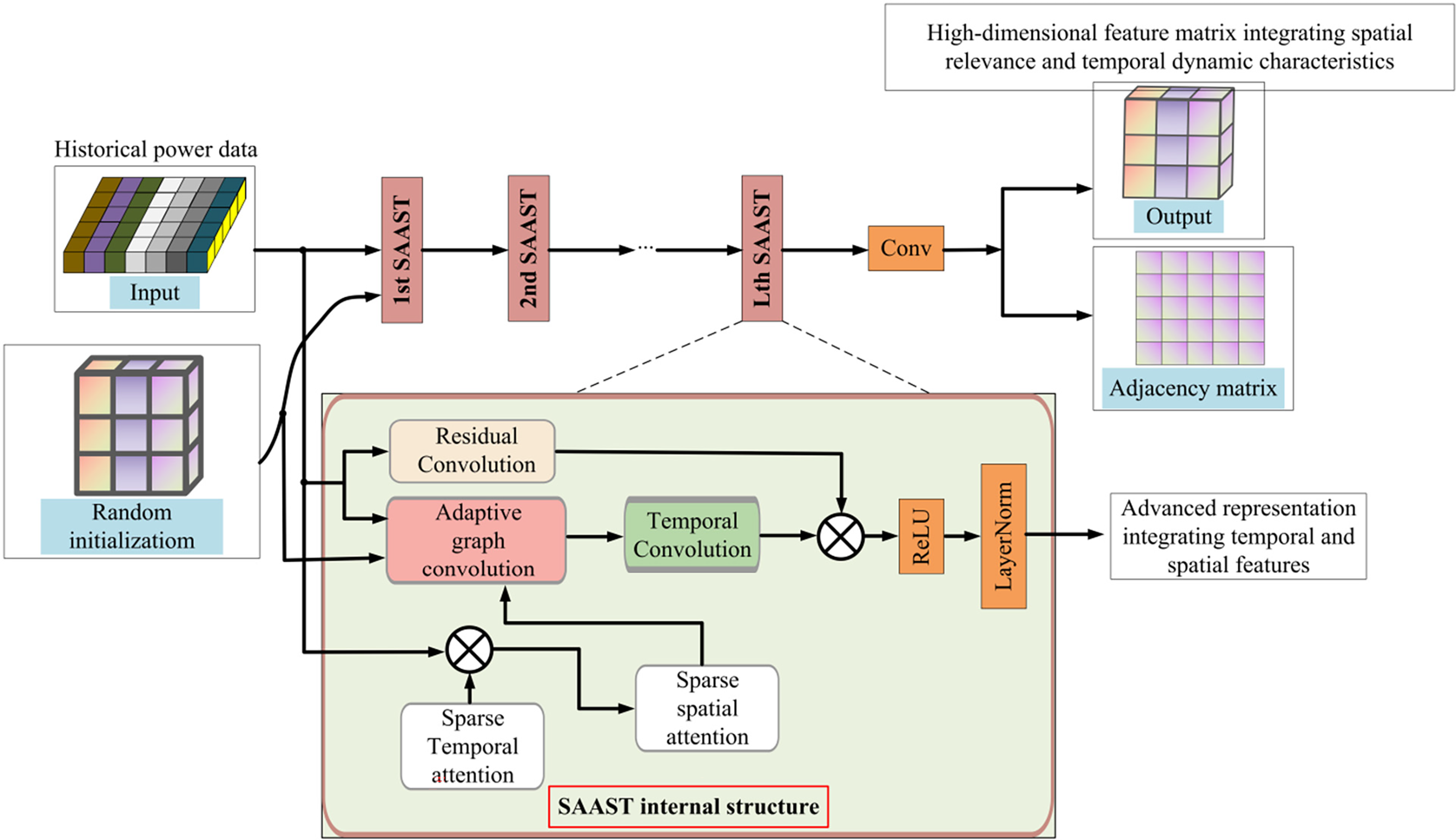
Figure 1: The proposed STGNN architecture

At the core of STGNN is the representation of PV stations as nodes in an undirected graph, where edges denote the correlations between stations. This graph-based structure enables the model to fully exploit spatial dependencies. To enhance modeling efficiency, sparse attention mechanisms are employed to filter out weak or irrelevant temporal and spatial correlations, allowing the model to focus on the most significant dependencies. This not only reduces computational complexity but also improves prediction performance.

STGNN consists of multiple Sparse Attention-based Adaptive Spatio-Temporal (SAAST) blocks. Each SAAST block integrates four key components: sparse temporal attention, sparse spatial attention, an adaptive GCN, and a TCN. The sparse temporal attention module captures meaningful temporal dependencies in historical power data by filtering out noise and low-relevance patterns. The sparse spatial attention module similarly evaluates inter-station spatial correlations, eliminating weak connections.

The adaptive GCN component dynamically learns an adjacency matrix during training, representing evolving spatial relationships among stations. This data-driven approach removes the reliance on manually defined graph structures and enables the model to extract latent spatial features more effectively.

Following spatial modeling, a TCN is applied to capture temporal dependencies by updating node features using information from preceding time steps. A residual convolution module is also incorporated to address gradient vanishing and other training challenges associated with deep architectures, thereby enhancing model stability and robustness.

In summary, STGNN integrates spatial and temporal modeling into a unified framework that effectively captures the spatio-temporal dynamics across multiple PV stations. Extensive experiments on real-world datasets demonstrate that the proposed model significantly outperforms baseline methods, highlighting its capability to model complex multi-site PV power generation patterns.

Dynamic Adaptive Mechanism: DEST-GNN uses a static graph structure relying on predefined node connections, while STGNN dynamically learns the adjacency matrix through adaptive GCN without prior topological knowledge, better fitting the dynamic correlations between distributed PV sites under changing weather conditions.

Sparse Attention Optimization: DEST-GNN does not introduce a sparse attention mechanism, whereas STGNN filters out weak correlations through Sparse Temporal Attention (STA) and Sparse Spatial Attention (SSA), significantly reducing computational complexity while improving feature learning efficiency.

3  Experiments and Analysis

Local solar irradiance data were collected from ten distinct sites and are presented in Fig. 2 (unit: W/m2). For experimental analysis, each PV system’s exact latitude and longitude coordinates were used to map its location; the geographical distribution of these ten systems is then illustrated in Fig. 3, with each site marked by a red symbol and labeled by its sensor identifier for clarity.

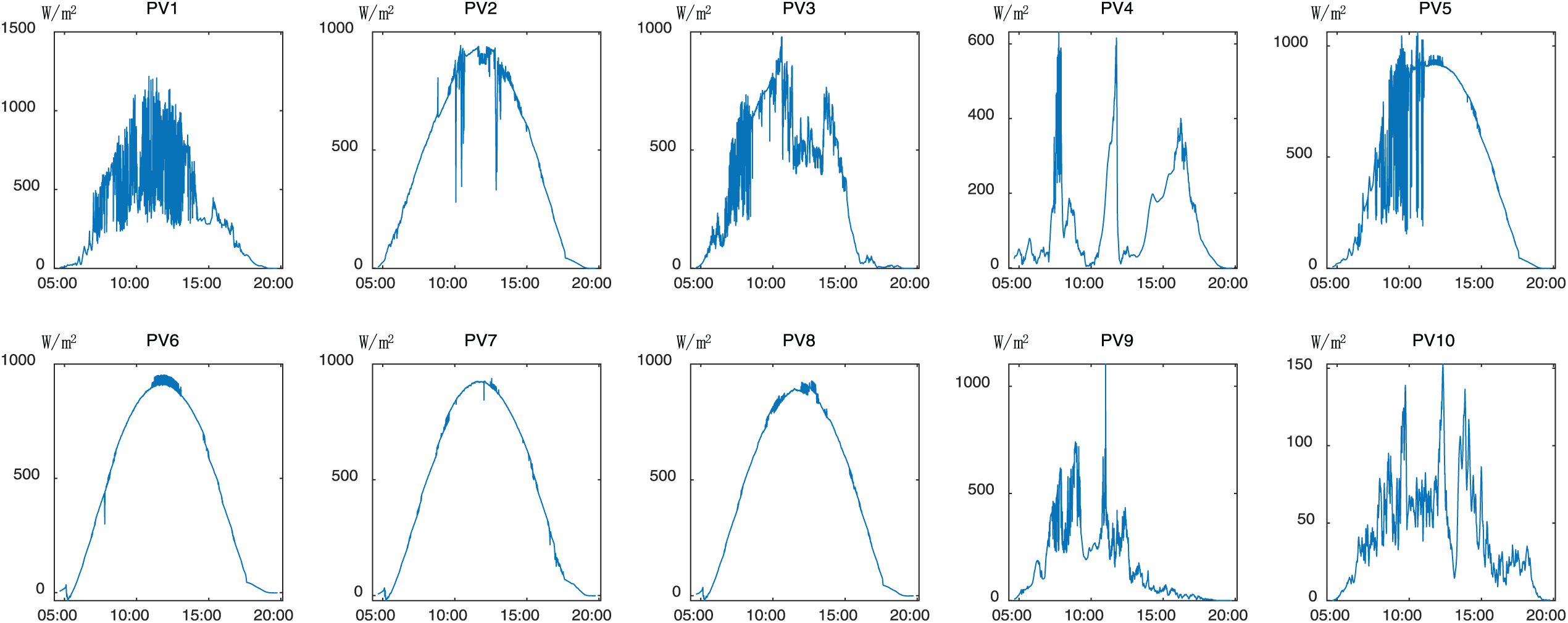
Figure 2: Solar irradiance measured from 05:00 to 20:00 on 04 April 2016

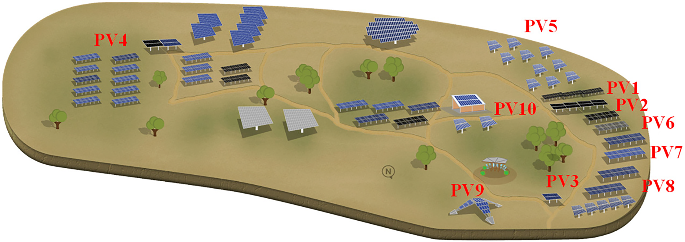
Figure 3: Geographic distribution of 10 distributed photovoltaic sampling points

3.1 Input Data Analysis and Preprocessing

The structure of the solar irradiance data can be represented as a matrix IR∈RT×M, with its mathematical form defined as follows:

IR=(ir1,1ir1,2⋯ir1,Mir2,1ir2,2⋯ir2,M⋮⋮⋮⋮irT,1irT,2⋯irT,M)(7)

In this study, IR is represented as a two-dimensional matrix, where M denotes the number of locations and T signifies the count of discrete time instances. Based on our data source, M is determined to be 10 for the case study. With a time resolution of 1 s and a test period spanning from 05:00:00 to 20:00:00, T is calculated to be 54,000, resulting in a 10 × 54,000 matrix as the input data.

Fig. 4 presents the results of the autocorrelation analysis for the recorded data, where the horizontal axis represents the lag and the vertical axis denotes the autocorrelation coefficient. A larger absolute value of the autocorrelation coefficient indicates a stronger autocorrelation property in the time series. For example, at PV1, data from most sites show significant autocorrelation. In contrast, the autocorrelation coefficients of local irradiance data at PV2 and PV8 are relatively low, which may constrain the accuracy of their respective prediction models. When multiple sites exhibit similar autocorrelation patterns, their data can be integrated to build a synergistic prediction model, thereby improving forecasting accuracy.

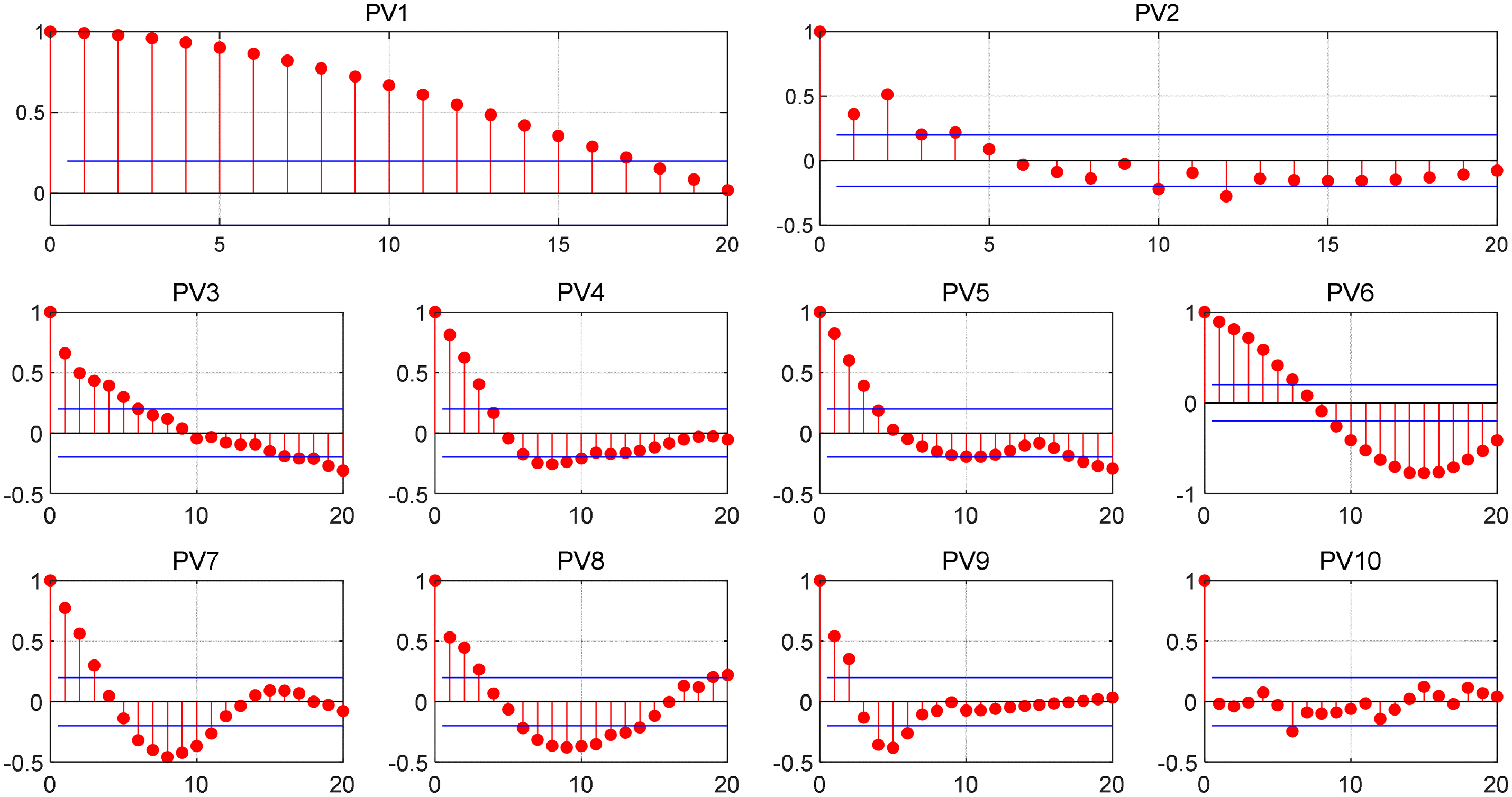
Figure 4: Autocorrelation analysis of data from 10 distributed photovoltaic systems

As shown in Fig. 5, spatial correlation analysis is employed to examine pattern similarities. The results reveal a notably high correlation between PV10 and PV2, despite their considerable geographical separation. This observation, together with the data in Figs. 3 and 5, confirms the theoretical analysis that correlations among distributed photovoltaic systems are not solely determined by physical distance. Typically, autocorrelation analysis highlights strong temporal dependencies, making it well-suited for time series forecasting. To improve data quality, Z-score normalization is applied to standardize the data to a normal distribution with a mean of 0 and a standard deviation of 1. For the input data matrix IR defined in Eq. (7), the mathematical formulation of Z-score normalization is given below:

irt,m∗=irt,m−μmσm(8)

where irt,m denotes any element in the original data IR, μm denotes the mean value of column m in IR, and σm denotes the standard deviation value of column m. A normalized form based on IR is constructed by replacing all irt,m with the normalized result irt,m∗. In the development of learning models, dataset division is a critical step, typically requiring the original dataset to be split into three independent subsets: training, validation, and test sets. In this study, the dataset is divided into training, validation, and test sets in a 7:2:1 ratio, which are utilized for model training, hyperparameter tuning, and performance evaluation, respectively.

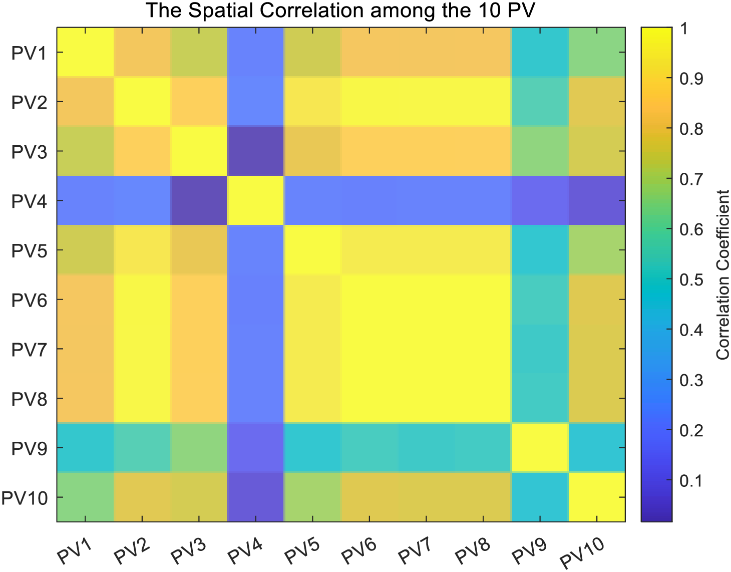
Figure 5: Spatial correlation map drawn based on PCC calculation results

In photovoltaic (PV) generation datasets, missing values may occur due to sensor faults or communication errors. To address this issue, the mean imputation method is employed. Given a dataset X = {x1, x2, …, xn}, where some data points xi are missing, each missing value is replaced using the mean of the available observations, as defined by the following formula.

xi=1n∑j=1nxj(9)

where n is the number of valid data for the feature, j denotes the serial number of the feature, and xj denotes the jth data point.

Outliers may be present in PV data due to measurement errors or abnormal operating conditions. To detect these, the Z-score method is applied. Each data point is standardized, and if its Z-score exceeds a specified threshold, it is classified as an outlier. The Z-score is calculated using the following formula.

Z=x−μσ(10)

where x denotes the value of the data point, μ is the mean of the feature, and σ is the standard deviation. A data point is identified as an outlier if |Z| > 3, and is subsequently processed accordingly.

3.2 Model Evaluation Metrics and Experimental Settings

The performance of the ST algorithm is evaluated and compared with other prediction methods. The evaluation metrics include overall prediction accuracy, training time, and error distribution characteristics. Prediction accuracy is quantified using three widely adopted metrics: Mean Absolute Error (MAE), Mean Absolute Percentage Error (MAPE), and Root Mean Square Error (RMSE). MAE (Eq. (11)) measures the average absolute difference between predicted and actual values; MAPE (Eq. (12)) expresses the relative error as a percentage; RMSE (Eq. (13)) emphasizes larger errors by squaring deviations, offering a more sensitive assessment of prediction fluctuations. Together, these metrics provide a comprehensive evaluation of the model’s predictive performance. The definitions of these metrics are as follows:

MAE=1N∑i=1N|yi^−yi|(11)

MAPE=1N∑i=1N|yi^−yiyi^|×100%(12)

RMSE=1N∑i=1N(yi^−yi)2(13)

where yi represents the ground truth, yi^ represents the predicted value of the model, and N represents the total number of samples. For a fair speed comparison, all tests were executed on a desktop computer equipped with an Intel i9-13900K CPU and an NVIDIA GeForce RTX 4090 GPU. The software environment comprised MATLAB 2022b and Python 3. The optimizer employs Root Mean Square Propagation (RMSProp), with the smoothing constant set to 0.99. The model’s hyperparameters are optimized based on training performance and graphical memory constraints. The specific hyperparameter settings are as follows: the batch size is set to 80 to balance training efficiency and memory consumption; the learning rate is set to 0.00001 to prevent excessive gradient fluctuations while ensuring model convergence. The K-hop size of the Graph Neural Network (GNN) is set to 2 to capture local neighborhood information. The sequence length and prediction length are set to 10 and 1, respectively, to accommodate time-series data characteristics, while the hidden state size of the LSTM network is configured as 80 × 10 to balance model expressiveness and computational complexity. The time step of the recurrent network is set to 10 to ensure effective modeling of temporal dependencies.

To ensure a fair and rigorous comparison, the baseline models, CNN+LSTM and GNN+LSTM, were re-implemented by us. We performed systematic hyperparameter tuning for these baselines to achieve their optimal performance on the validation set.

For CNN+LSTM: Our implementation followed the canonical CNN+LSTM architecture prevalent in the literature. For the CNN component, key hyperparameters, including the quantity and dimensionality of convolutional kernels, as well as pooling layer configurations, were systematically optimized. The architecture employed a progressive design where the convolutional layers began with 32 filters in the initial shallow layers, gradually increasing to 128 filters in deeper layers. All convolutional kernels maintained a consistent 3 × 3 spatial dimension throughout the network. For dimensionality reduction, Max Pooling layers were exclusively implemented, each configured with a 2 × 2 pooling window and a stride of 2.

For the LSTM component, key parameters such as hidden unit dimensions and time steps were aligned with our STGNN model’s temporal processing module or adjusted according to recommended values in established literature. Specifically, the hidden state dimension was set to 80 × 10 and the time steps to 10 (consistent with the details in Section 3.2 of our manuscript).

For GNN+LSTM: Similarly, our GNN+LSTM implementation adhered to standard architectures in the field. For the GNN component, the K-hop size was set to 2 (as specified in Section 3.2). The graph convolutional layers were configured with 64 hidden units, and their output dimension feeding into the LSTM was set to 7. The LSTM component in the GNN+LSTM model employed the same hyperparameter settings and optimization strategy as that in the CNN+LSTM model, particularly regarding hidden state dimensions and time steps.

Both baseline models were trained using the RMSProp optimizer with a learning rate of 0.00001 and a batch size of 80, consistent with the training of our proposed STGNN model. The same training, validation, and test set splits (7:2:1 ratio) were used for all models, and performance was evaluated using identical metrics (MAE, MAPE, RMSE) to guarantee fairness.

3.3 Training Process

The optimal model was selected based on a thorough accuracy analysis, and its training process was comprehensively evaluated. Fig. 6 illustrates the dynamic changes in validation loss, measured by Mean Squared Error (MSE), over the training epochs for the three best-performing deep learning models. The horizontal axis represents the training epochs, indicating the number of iterations during which the model learns from the training data [40]. Comparative analysis shows that the validation loss of all three models gradually decreases with increasing epochs, reflecting improved generalization and enhanced prediction accuracy [41]. Notably, as shown in Fig. 6, the proposed STGNN model achieves the lowest validation loss more rapidly than the other models, demonstrating superior training efficiency and predictive performance.

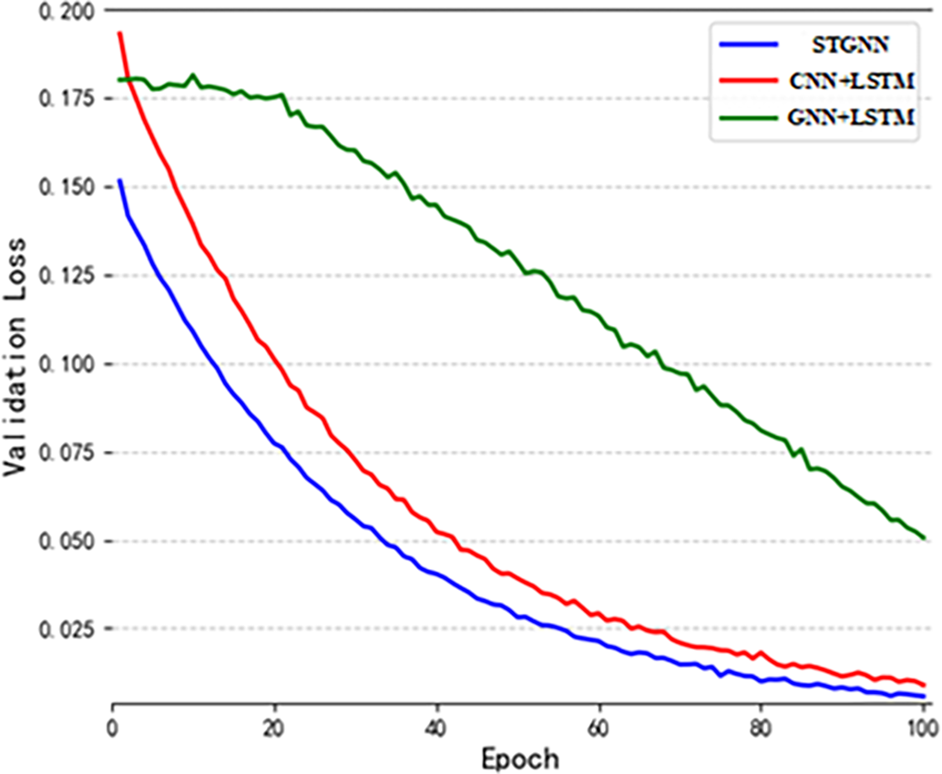
Figure 6: Dynamic training process of three algorithms

3.4 Comparative Analysis

Table 1 summarizes the prediction performance comparison across models, reporting MAE, MAPE, and RMSE values. Both composite models and the proposed STGNN demonstrate strong predictive capabilities. Notably, the STGNN model achieves the lowest errors across all three metrics, significantly outperforming the other evaluated models [42]. Furthermore, the integration of sparse attention mechanisms, such as those in the SAAST modules, provides STGNN with a clear advantage over models relying on conventional dense attention.

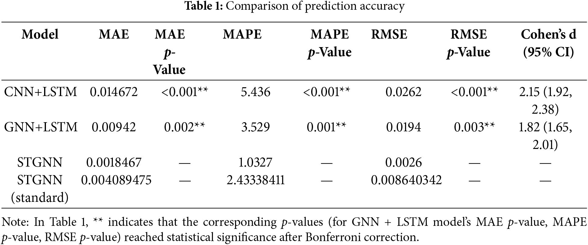
Fig. 7 presents detailed prediction results of the proposed STGNN model, alongside those of the CNN+LSTM and GNN+LSTM models. The horizontal axis represents consecutive time points, while the vertical axis shows the corresponding actual and predicted standardized solar irradiance fluctuations. The figure consists of 10 subplots, each corresponding to one of the sensing stations shown in Fig. 3. Across all three models, predicted values generally align well with the actual measurements. However, the STGNN predictions, highlighted as the top trend line, demonstrate closer adherence to true values compared to CNN+LSTM and GNN+LSTM, indicating superior accuracy and distribution consistency. For robustness verification, paired t-tests (parametric) and Wilcoxon signed-rank tests (non-parametric) were conducted, with Bonferroni correction applied to control the family-wise error rate (adjusted α = 0.0033). The RMSE difference between GNN+LSTM and STGNN yields p = 0.0030, approaching the Bonferroni-adjusted threshold (α = 0.0033). Despite this marginality, the effect size d = 1.82 (95% CI: 1.65–2.01) substantially exceeds the conventional large-effect threshold (d > 0.8), confirming practical significance. To further validate, we computed Kolmogorov-Smirnov statistic D = 0.38 (p < 0.001) for error distributions, rejecting the null hypothesis of identical distributions. Statistical analysis confirms that STGNN significantly outperforms all baseline models (p < 0.0033, Cohen’s d > 1.8), demonstrating both statistical significance and practical engineering relevance.

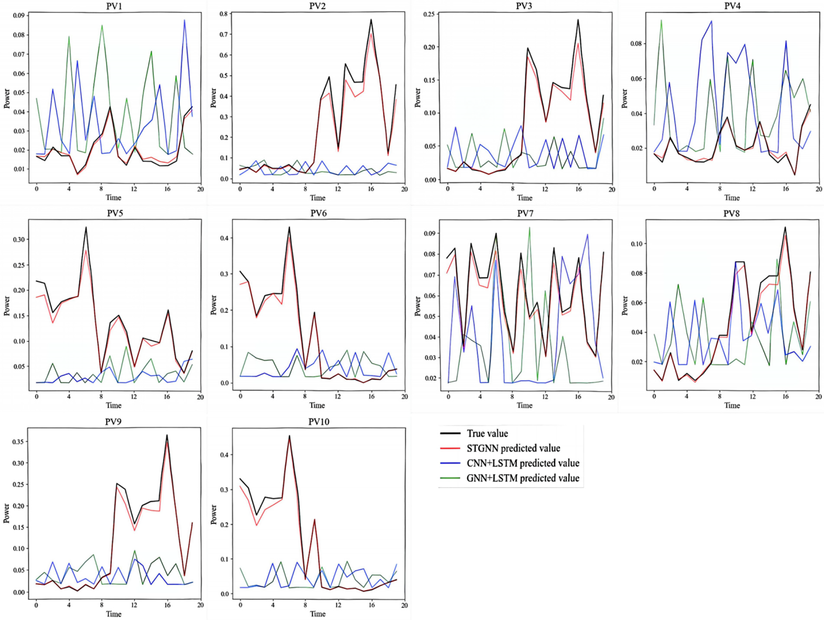
Figure 7: Comparison of prediction results between STGNN and other models

In addition to the DKASC dataset, experiments and analyses were conducted on another photovoltaic dataset, further demonstrating the superiority of the proposed model over competing approaches.

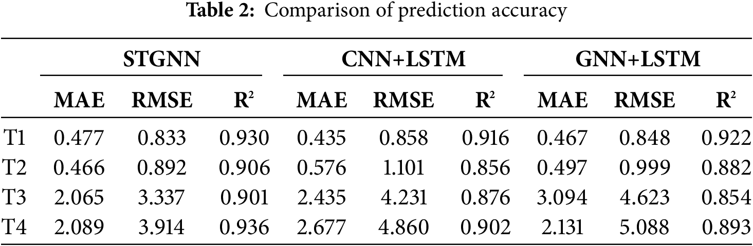
The second dataset is the Guoneng Rising PV Power Forecast Competition dataset, which includes environmental data and power generation records from four distributed PV power plants. The four PV power plants are located in different regions of China, with a data resolution of 15 min and a time span from January 2017 to December 2017. From the experimental results in Fig. 8, it can be seen that the MAE, RMSE and R2 of STGNN outperform the baseline model in all four power plants from T1–T4, which proves the generalization ability of the model.

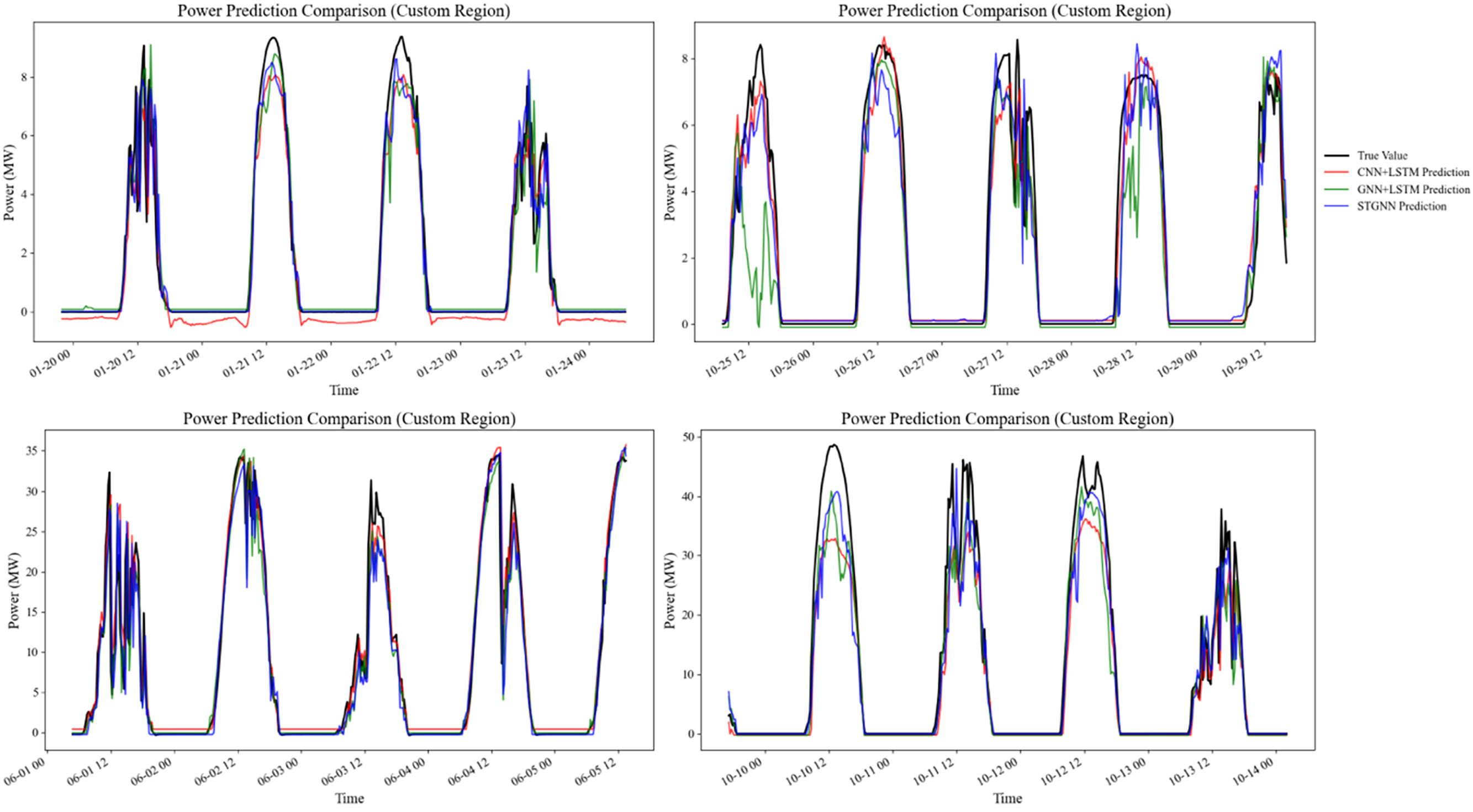
Figure 8: Comparison of prediction results between STGNN and other models

The comparison of prediction accuracy is presented in Table 2.

It is noteworthy that the overall time complexity of the STGNN model is predominantly determined by its core architectural components: spatiotemporal graph convolution (GCN), temporal convolutional modules (TCN), and sparse attention mechanisms. Assuming an input sequence length of T, M nodes, C channels, D neighbors per GCN layer, a TCN kernel size of K, and L network layers. Throughout the experimental procedure, the input sequence parameters were configured as follows: sequence length T = 10, nodes M = 10, channel size C = 64. The parameter D, representing the adaptive graph convolutional network’s dynamic dimensionality, is not a fixed value due to the model’s utilization of Adaptive GCN. For analytical purposes, we consider its worst-case scenario where D = 9. Additional architectural parameters include K = 3 and L = 3. The computational complexity can be characterized as follows:

1.    Spatiotemporal Graph Convolution (GCN): Each layer exhibits a complexity of O(M×D×C2). The adaptive GCN optimizes neighbor interactions through dynamic adjacency matrices, thereby reducing computational redundancy.

2.    Temporal Convolution (TCN): Each layer demonstrates a complexity of O(T×K×C2). Dilated convolutions facilitate exponential receptive field expansion to capture long-term dependencies, while computational demands increase linearly with the number of layers L.

3.    Sparse Attention Mechanism: By filtering weak spatiotemporal correlations, this mechanism reduces complexity from O(M2×T) to O(S×M×T), where S≪M represents the number of effectively correlated nodes, substantially diminishing inefficient computations.

4.    Residual Connections: These require merely O(T×C) addition operations, rendering their computational overhead negligible.

The total computational complexity can be expressed as Eq. (14), where TCN and GCN convolution operations constitute the main computational load. In real-time applications, the STGNN architecture leverages sparse attention mechanisms (with sparsity S≪M) and dynamic pruning via adaptive GCN, achieving high predictive accuracy while maintaining computational efficiency. The single-step prediction latency ranges from 0.52164 to 1.25265 s, confirming the model’s practical viability for real-time forecasting scenarios.

O(L×(M×D×C2+T×K×C2+S×M×T))(14)

In summary, the experimental results demonstrate that the proposed STGNN framework achieves superior prediction accuracy and robustness in solar irradiance forecasting for distributed PV systems.

3.5 Ablation Analysis of STGNN Components

To elucidate the contributions of each core component in our STGNN architecture, we performed the following ablation studies under identical training conditions and hyperparameters:

STGNN w/o STA (without Sparse Temporal Attention): The STA module was omitted, such that temporal representations produced by the SAAST block were passed directly to the Temporal Convolutional Network (TCN) without any attention-based temporal weighting.

STGNN w/o SSA (without Sparse Spatial Attention): The SSA module was removed, and graph convolutions were applied to spatial features in the absence of an attention mechanism for emphasizing salient neighboring nodes.

STGNN w/o Adaptive GCN (without Adaptive Graph Convolutional Network): The adaptive Graph Convolutional Network—responsible for learning the adjacency matrix dynamically—was replaced with a static GCN. The static adjacency matrix was predefined according to pairwise physical distances among sites, while all other architectural components and training protocols remained unchanged.

The ablation study results are presented in Table 3.

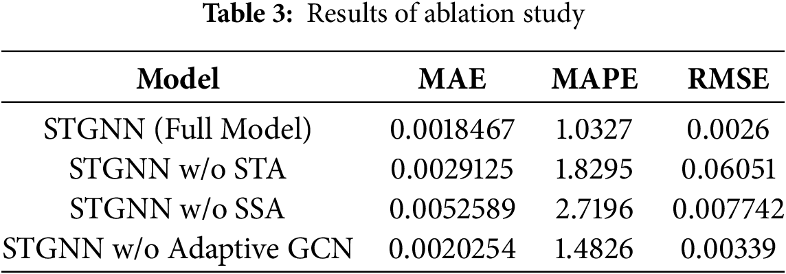
As summarized in Table 3, omitting the STA module (STGNN w/o STA) incurs a 57% increase in MAE and a 22-fold rise in RMSE. In contrast, removing SSA module (STGNN w/o SSA) produces even larger degradations in both metrics. This discrepancy reflects the differing natures of temporal vs. spatial dependencies in photovoltaic power forecasting. Temporal correlations between stations are intermittent—becoming pronounced mainly during abrupt weather changes—whereas spatial correlations, dictated by fixed geographic layouts, remain consistently strong. Hence, the absence of STA yields moderate error increases, but the lack of SSA significantly undermines predictive accuracy, underscoring the necessity of sparse spatio-temporal attention to both capture salient patterns and attenuate noise.

Moreover, replacing the Adaptive GCN with a static GCN has only a marginal impact on error metrics. The adaptive GCN dynamically learns the graph topology—allowing the average neighbor count D to be determined during training and potentially approach full connectivity (i.e., D→9 for our nine-station network). In our ablation, we fixed D = 9 for the static GCN to emulate this worst-case connectivity. Although predictive performance remains largely unaffected, inference latency increases noticeably: single-step forecasting runtimes rise to 0.649–1.439 s, representing approximately a 15% extension over the full STGNN model.

4  Conclusions

This study proposes a novel STGNN architecture specifically designed for distributed photovoltaic power forecasting. The framework integrates an innovative SAAST module for joint spatio-temporal feature extraction. The sparse attention mechanism effectively filters out irrelevant correlations, enhancing pattern recognition in power generation data. An adaptive spectral graph convolution operator autonomously learns inherent spatial dependencies from measurement data, eliminating the reliance on predefined topologies.

Complemented by a temporal convolution module [43], the architecture captures dynamic, time-varying characteristics across multi-site PV generation sequences. To enhance computational robustness and ensure network convergence stability, a residual connection mechanism is incorporated. Comprehensive evaluations based on the DKASC dataset and an additional photovoltaic dataset demonstrate that the proposed STGNN significantly outperforms benchmark forecasting algorithms in terms of generalization capability, reliability, and prediction accuracy [44]. These performance advantages are substantiated through multi-dimensional comparative experiments, with quantifiable improvements explicitly visualized.

This method addresses the critical need for accurate and robust forecasting models tailored for distributed PV systems. By modeling each PV installation as a node in a graph and learning adaptive spatial relationships among power outputs, the STGNN framework provides a scalable and generalizable solution for large-scale PV integration into power grids. Its ability to adapt to local variations while maintaining predictive accuracy across multiple sites makes it highly valuable for grid operators aiming to enhance renewable energy integration and ensure system stability.

Acknowledgement: The authors would like to thank the China Electric Power Research Institute and the State Grid Company Limited for providing useful infrastructure and support for carrying out various studies related to this paper.

Funding Statement: The research is supported by the State Grid Corporation of China Headquarters Science and Technology Project “Research on Key Technologies for Power System Source-Load Forecasting and Regulation Capacity Assessment Oriented towards Major Weather Processes” (4000-202355381A-2-3-XG).

Author Contributions: The authors confirm contribution to the paper as follows: Research concept and design: Dayan Sun and Zhifeng Liang; Data collection: Junrong Xia and Yuqi Wang; Model construction and experimental verification: Xiao Cao. All authors reviewed the results and approved the final version of the manuscript.

Availability of Data and Materials: Not applicable.

Ethics Approval: Not applicable.

Conflicts of Interest: The authors declare no conflicts of interest to report regarding the present study.

References

1. Kroposki B, Johnson B, Zhang Y, Gevorgian V, Denholm P, Hodge BM, et al. Achieving a 100% renewable grid: operating electric power systems with extremely high levels of variable renewable energy. IEEE Power Energy Mag. 2017;15(2):61–73. doi:10.1109/mpe.2016.2637122. [Google Scholar] [CrossRef]

2. Zhang D, Feng KH, Shi ZY, Yu QX. Current states and recommendations for grid integration of new energy in China. Sol Energy. 2024(7):89–97. (In Chinese). doi:10.19911/j.1003-0417.tyn20240605.03. [Google Scholar] [CrossRef]

3. Yang X, Song Y, Wang G, Wang W. A comprehensive review on the development of sustainable energy strategy and implementation in China. IEEE Trans Sustain Energy. 2010;1(2):57–65. doi:10.1109/TSTE.2010.2051464. [Google Scholar] [CrossRef]

4. Liu XY, Wang J, Yao TC, Zhang P, Chi XB. Ultra short-term distributed photovoltaic power prediction based on satellite remote sensing. Trans China Electrotech Soc. 2022;37(7):1800–9. (In Chinese). doi:10.19595/j.cnki.1000-6753.tces.210311. [Google Scholar] [CrossRef]

5. Liu X, Xie X, Fang Q, Xu F, Huang C, Zhen Z, et al. Spatial-temporal attention mechanism and graph convolutional networks based distributed PV ultra-short-term power forecasting. In: Proceedings of the 2023 IEEE International Conference on Energy Technologies for Future Grids (ETFG); 2023 Dec 3–6; Wollongong, Australia. doi:10.1109/ETFG55873.2023.10408590. [Google Scholar] [CrossRef]

6. Hua K, Simovici DA. Long-lead term precipitation forecasting by hierarchical clustering-based bayesian structural vector autoregression. In: Proceedings of the 2016 IEEE 13th International Conference on Networking, Sensing and Control (ICNSC); 2016 Apr 28–30; Mexico City, Mexico. doi:10.1109/ICNSC.2016.7479002. [Google Scholar] [CrossRef]

7. Xu Q, Ding K, Xu M, Wang X, Li T, Liu Z. Short-term wind power prediction for extreme weather scenarios based on tensor autoregression completion algorithm and ARMA error correction. In: Proceedings of the 2024 Boao New Power System International Forum—Power System and New Energy Technology Innovation Forum (NPSIF); 2024 Dec 8–10; Qionghai, China. doi:10.1109/NPSIF64134.2024.10883599. [Google Scholar] [CrossRef]

8. Gharehbagh HK, Jalalat SM, Agabalaye-Rahvar M, Zare K, Gözel T. Residential electricity demand forecasting employing a highly accurate BiLSTM intelligent model. In: Proceedings of the 2024 9th International Conference on Technology and Energy Management (ICTEM); 2024 Feb 14–15; Behshar, Islamic Republic of Iran. doi:10.1109/ICTEM60690.2024.10631923. [Google Scholar] [CrossRef]

9. Han F, Pu T, Li M, Taylor G. Short-term forecasting of individual residential load based on deep learning and K-means clustering. CSEE J Power Energy Syst. 2020;7(2):261–9. doi:10.17775/CSEEJPES.2020.04060. [Google Scholar] [CrossRef]

10. Huang Y, Zhang Y, Zhao Y, Shi P, Chambers JA. A novel outlier-robust Kalman filtering framework based on statistical similarity measure. IEEE Trans Autom Control. 2021;66(6):2677–92. doi:10.1109/tac.2020.3011443. [Google Scholar] [CrossRef]

11. Hanene C, Abdelhamid I, Kouider L, Ahmed H. Maximum power point tracking based extended Kalman filter. In: Proceedings of the 2023 Second International Conference on Energy Transition and Security (ICETS); 2023 Dec 12–14; Adrar, Algeria. doi:10.1109/ICETS60996.2023.10410734. [Google Scholar] [CrossRef]

12. Firouzi H, Hero AO, Rajaratnam B. Two-stage sampling, prediction and adaptive regression via correlation screening. IEEE Trans Inf Theory. 2017;63(1):698–714. doi:10.1109/TIT.2016.2621111. [Google Scholar] [CrossRef]

13. Selvi MV, Mishra S. Investigation of performance of electric load power forecasting in multiple time horizons with new architecture realized in multivariate linear regression and feed-forward neural network techniques. IEEE Trans Ind Appl. 2020;56(5):5603–12. doi:10.1109/TIA.2020.3009313. [Google Scholar] [CrossRef]

14. Cao W, Mei D, Guo Y, Ghorbani H. Deep learning approach to prediction of drill-bit torque in directional drilling sliding mode: energy saving. Measurement. 2025;250(4):117144. doi:10.1016/j.measurement.2025.117144. [Google Scholar] [CrossRef]

15. Zhuang J, Cao Y, Ding Y, Jia M, Feng K. An autoregressive model-based degradation trend prognosis considering health indicators with multiscale attention information. Eng Appl Artif Intell. 2024;131:107868. doi:10.1016/j.engappai.2024.107868. [Google Scholar] [CrossRef]

16. Fei X, Ling Q. Attention-based global and local spatial-temporal graph convolutional network for vehicle emission prediction. Neurocomputing. 2023;521(3):41–55. doi:10.1016/j.neucom.2022.11.085. [Google Scholar] [CrossRef]

17. Yu C, Yan G, Yu C, Zhang Y, Mi X. A multi-factor driven spatiotemporal wind power prediction model based on ensemble deep graph attention reinforcement learning networks. Energy. 2023;263(2):126034. doi:10.1016/j.energy.2022.126034. [Google Scholar] [CrossRef]

18. Zheng C, Fan X, Wang C, Qi J. GMAN: a graph multi-attention network for traffic prediction. In: Proceedings of the AAAI Conference on Artificial Intelligence; 2020 Feb 7–12; New York, NY, USA. doi:10.1609/aaai.v34i01.5477. [Google Scholar] [CrossRef]

19. Liu Y, Liu Q, Zhang JW, Feng H, Wang Z, Zhou Z, et al. Multivariate time-series forecasting with temporal polyno-mial graph neural networks. Adv Neural Inf Process Syst. 2022;35:19414–26. [Google Scholar]

20. Han L, Du B, Sun L, Fu Y, Lv Y, Xiong H. Dynamic and multi-faceted spatio-temporal deep learning for traffic speed forecasting. In: Proceedings of the 27th ACM SIGKDD Conference on Knowledge Discovery & Data Mining; 2021 Aug 14–18; Virtual Event, Singapore. doi:10.1145/3447548.3467275. [Google Scholar] [CrossRef]

21. Song D, Rehman MSU, Deng X, Xiao Z, Noor J, Yang J, et al. Accurate solar power prediction with advanced hybrid deep learning approach. Eng Appl Artif Intell. 2025;148(12):110367. doi:10.1016/j.engappai.2025.110367. [Google Scholar] [CrossRef]

22. Sukanya G, Priyadarshini J. Fine tuned hybrid deep learning model for effective judgment prediction. Comput Model Eng Sci. 2025;142(3):2925–58. doi:10.32604/cmes.2025.060030. [Google Scholar] [CrossRef]

23. Işık C, Kuziboev B, Ongan S, Saidmamatov O, Mirkhoshimova M, Rajabov A. The volatility of global energy uncertainty: renewable alternatives. Energy. 2024;297(5):131250. doi:10.1016/j.energy.2024.131250. [Google Scholar] [CrossRef]

24. Zhao ZB, Qiang YF, Li X, Xiao N, Li J, Xi YN, et al. Ultra-short-term power prediction method of distribution network based on improved recurrent neural network. J Electr Power Sci Technol. 2022;37(5):144–54. (In Chinese). doi:10.19781/j.issn.1673-9140.2022.05.016. [Google Scholar] [CrossRef]

25. Bayrak F. Prediction of photovoltaic panel cell temperatures: application of empirical and machine learning models. Energy. 2025;323:135764. doi:10.1016/j.energy.2025.135764. [Google Scholar] [CrossRef]

26. Meng A, Zhang H, Yin H, Xian Z, Chen S, Zhu Z, et al. A novel multi-gradient evolutionary deep learning approach for few-shot wind power prediction using time-series GAN. Energy. 2023;283:129139. doi:10.1016/j.energy.2023.129139. [Google Scholar] [CrossRef]

27. Yang X, Guo X, Chen C, Xie M, Zhang J, Shu J. Research on short-term power load forecasting method based on CEEMDAN-ChOA-GRU. In: Proceedings of the 2023 IEEE International Conference on Energy Technologies for Future Grids (ETFG); 2023 Dec 3–6; Wollongong, Australia. doi:10.1109/ETFG55873.2023.10407106. [Google Scholar] [CrossRef]

28. Gui X, Tan L, Huang Y. A study of a photovoltaic power prediction method combining BiLSTM and GWO. In: Proceedings of the 2024 5th International Conference on Computer Engineering and Application (ICCEA); 2024 Apr; Hangzhou, China. doi:10.1109/ICCEA62105.2024.10604113. [Google Scholar] [CrossRef]

29. Dhaked DK, Dadhich S, Birla D. Power output forecasting of solar photovoltaic plant using LSTM. Green Energy Intell Transp. 2023;2(5):100113. doi:10.1016/j.geits.2023.100113. [Google Scholar] [CrossRef]

30. Guo Z, Zhao F, Wang B, Xu W, Zhang T, Guo K. Medium to long term wind power prediction based on improved mRMR algorithm and GWO-LSTM algorithm. In: 2024 6th International Conference on Energy Systems and Electrical Power (ICESEP); 2024 Jun 21–23; Wuhan, China. doi:10.1109/ICESEP62218.2024.10651978. [Google Scholar] [CrossRef]

31. Wang S, Zhang Y, Wang Z, Cui F, Wang S. A power prediction method for PV system based on wavelet decomposition and neural networks. In: Proceedings of the 2020 IEEE/IAS Industrial and Commercial Power System Asia (I&CPS Asia); 2020 Jul 13–15; Weihai, China. doi:10.1109/icpsasia48933.2020.9208483. [Google Scholar] [CrossRef]

32. Dong H, He H, Hu S, Tang P, Zhang X. Short-term electrical load forecasting based on whale optimized variational mode decomposition and DCNN-BiLSTM. In: Proceedings of the 2023 15th International Conference on Communication Software and Networks (ICCSN); 2023 Jul 21–23; Shenyang, China. doi:10.1109/ICCSN57992.2023.10297380. [Google Scholar] [CrossRef]

33. Chen X, Yang L, Liu Y. Research on negative charge prediction method based on deep learning. In: Proceedings of the 2024 8th International Conference on Power Energy Systems and Applications (ICoPESA); 2024 Jun 24–26; Hong Kong, China. doi:10.1109/ICOPESA61191.2024.10743904. [Google Scholar] [CrossRef]

34. Sun F, Li L, Bian D, Bian W, Wang Q, Wang S. Photovoltaic power prediction based on multi-scale photovoltaic power fluctuation characteristics and multi-channel LSTM prediction models. Renew Energy. 2025;246:122866. doi:10.1016/j.renene.2025.122866. [Google Scholar] [CrossRef]

35. Zhao M, Li S, Chen H, Ling M, Chang H. Distributed solar photovoltaic power prediction algorithm based on deep neural network. J Eng Res. 2024;37(2):S230718772400316X. doi:10.1016/j.jer.2024.12.013. [Google Scholar] [CrossRef]

36. Yang Y, Liu Y, Zhang Y, Shu S, Zheng J. DEST-GNN: a double-explored spatio-temporal graph neural network for multi-site intra-hour PV power forecasting. Appl Energy. 2025;378:124744. doi:10.1016/j.apenergy.2024.124744. [Google Scholar] [CrossRef]

37. Zhao Y, Pu H, Dai Y, Cong S. Short-term wind power prediction method based on GCN-LSTM. In: Proceedings of the 2023 8th Asia Conference on Power and Electrical Engineering (ACPEE); 2023 Apr 14–16; Tianjin, China. doi:10.1109/ACPEE56931.2023.10135621. [Google Scholar] [CrossRef]

38. Fan M, Peng Y, Zhang H. Photovoltaic output power prediction model based on K-GCN-LSTM neural network. In: 2024 36th Chinese Control and Decision Conference (CCDC); 2024 May 25–27; Xi’an, China. doi:10.1109/CCDC62350.2024.10587628. [Google Scholar] [CrossRef]

39. Zolfaghari S, Hossein Hasheminejad SM. Generalized self-attentive spatiotemporal GCN with OPTICS clustering for recommendation systems. In: Proceedings of the 2024 15th International Conference on Information and Knowledge Technology (IKT); 2024 Dec 24–26; Isfahan, Islamic Republic of Iran. doi:10.1109/IKT65497.2024.10892621. [Google Scholar] [CrossRef]

40. Shen X, Ji C, Lai X, Zhao L, Jiang S. Energy-STGNN: a dynamic forecasting approach for energy consumption prediction. In: Proceedings of the 2024 10th IEEE International Conference on Intelligent Data and Security (IDS); 2024 May 10–12; New York, NY, USA. doi:10.1109/IDS62739.2024.00022. [Google Scholar] [CrossRef]

41. Cheng Z, Zhou Y, Zhang J, Li Y, Deng Y, Tan S, et al. Photovoltaic power generation power prediction method based on digital twins and deep learning. In: Proceedings of the 2023 5th International Conference on Electrical Engineering and Control Technologies (CEECT); 2023 Dec 15–17; Chengdu, China. doi:10.1109/CEECT59667.2023.10420619. [Google Scholar] [CrossRef]

42. Yoon H, Chon KW, Kim MS. FedSTGNN: a federated spatio-temporal graph neural network. In: Proceedings of the 2024 15th International Conference on Information and Communication Technology Convergence (ICTC); 2024 Oct 16–18; Jeju Island, Republic of Korea. doi:10.1109/ICTC62082.2024.10826762. [Google Scholar] [CrossRef]

43. Zhou X, Pang C, Zeng X, Jiang L, Chen Y. A short-term power prediction method based on temporal convolutional network in virtual power plant photovoltaic system. IEEE Trans Instrum Meas. 2023;72:9003810. doi:10.1109/TIM.2023.3301904. [Google Scholar] [CrossRef]

44. Li L, Zhou X, Hu G, Li S, Jia D. A recurrent spatio-temporal graph neural network based on latent time graph for multi-channel time series forecasting. IEEE Signal Process Lett. 2024;31:2875–9. doi:10.1109/LSP.2024.3479917. [Google Scholar] [CrossRef]