
 Submit a Paper
 Propose a Special lssue
 Open Access
ARTICLE

A Fault Location Method of Multi-Branch Distribution Line Based on MODWT Combined with Improved TEO
School of Automation, Chongqing University of Posts and Telecommunications, Chongqing, 400065, China
* Corresponding Author: Pan Duan. Email:
Energy Engineering 2025, 122(9), 3817-3838. https://doi.org/10.32604/ee.2025.066491
Received 09 April 2025; Accepted 23 June 2025; Issue published 26 August 2025
 View Full Text
 Download PDF
Abstract
To address the challenges of fault line identification and low detection accuracy of wave head in Fault Location (FL) research of distribution networks with complex topologies, this paper proposes an FL method of Multi-Branch distribution line based on Maximal Overlap Discrete Wavelet Transform (MODWT) combined with the improved Teager Energy Operator (TEO). Firstly, the current and voltage Traveling Wave (TW) signals at the head of each line are extracted, and the fault-induced components are obtained to determine the fault line by analyzing the polarity of the mutation amount of fault voltage and current TWs. Subsequently, the fault discrimination mark is calculated based on the fault-induced line-mode current and the zero-mode voltage, with the fault type determined by comparing each mark’s value against the fault discrimination table, transforming the FL problem in complex topology into a single-line FL problem. Finally, the fault voltage TW is extracted from the fault line, and the wave head detection method based on MODWT combined with improved TEO is used to precisely identify the arrival instants of both the first TW wave head and its first reflection at each line terminal, and then the FL result is calculated by applying the double-ended TW ranging formula that removes the influence of wave velocity. Simulation results demonstrate that the proposed method accurately identifies the fault line and types of faults occurring and maintains the ranging accuracy within 0.5% under various fault scenarios.Keywords
As modern power grids evolve, distribution networks, serving as the critical link between the grid side and load side, play a pivotal role in ensuring reliable power supply for social production and residential life. Statistics indicate that distribution line faults account for about 80% of grid faults [1]. Distribution networks typically feature numerous branches and complex structures, making the traditional manual patrolling method difficult and inefficient, which cannot fulfill the demands of modern power systems for swift electricity restoration. Given the unpredictable nature of fault occurrences, the rapid and accurate identification of fault points can significantly reduce inspection time, accelerate the fault processing cycle, and enhance the operational stability and security of the power system [2].
Due to the multi-branch topology characteristic of distribution networks, the fault branches must be determined before the fault point is accurately located. Previous studies have proposed various approaches to address this challenge: Literature [3] establishes fault branching criteria by analyzing the length of each branch and the arrival time of the fault TW at each measurement end. However, this method is only applicable to T-connected lines. With the increasing complexity of modern distribution network topologies, to accommodate increasingly complex distribution network topologies, literature [4] establishes the topology describing the matrix of the distribution network based on the matrix method, and when a fault occurs, fault branching is determined by using the data of the fault indicator. However, the fault indicator is easily misjudged in practical engineering due to the failure of directional components [5]. Based on this problem, literature [6] transfers the omission and false alarm variables to offline identification, thereby avoiding direct reliance on potentially unreliable data in real-time calculations and improving the stability of localization results. However, the method does not apply to all operational scenarios in distribution networks. Another Literature [7] proposes a fault section location method by fusing remote fault indicators, smart meters, and distributed phasor measurement unit data. However, it is difficult to achieve multisource data fusion in existing distribution network equipment. Therefore, current research on fault line identification has certain limitations.
FL methods are primarily divided into two categories: the impedance method and the TW method [8]. The impedance method is based on the principle that the distance between the measuring end and the fault point is proportional to the impedance, and the fault distance is estimated by the impedance of the fault circuit based on the collected voltage and current [9], and the data belongs to the steady state quantity of the industrial frequency, which has the advantage of low cost of realization in the practical engineering. However, the impedance method has certain defects in principle; the algorithm is usually based on assumptions, and at the same time, it is easily affected by system operating conditions, fault resistance, and other variables that affect distance measurement accuracy [10].
The TW method is a diagnostic technique that utilizes wave propagation dynamics for fault identification through the analysis of TW propagation time in the line, refraction characteristics, and waveform change characteristics to achieve FL [11]. The accuracy of this approach primarily depends on two parameters: the arrival time of TW at monitoring terminals and the propagation velocity [12]. To address the problem of wave head time detection, the TW method often employs a signal decomposition algorithm for signal processing to obtain the signal in both the time and frequency domains, as well as other multi-scale features. Literature [13] employed Discrete Wavelet Transform (DWT) for wave head detection. However, DWT may cause information loss and spectral aliasing during down-sampling operation, and the transform result is sensitive to wavelet basis selection and decomposition scale. Literature [14] extracted the faulty signal features based on the Hilbert-Huang Transform (HHT) and accurately computed the TW arrival moments to determine the FL through the sampling error correction method. However, the HHT has the problem of modal aliasing, which can obscure wave head features and potentially cause misjudgment. Based on this problem, literature [15] proposed an improved approach using adaptive noise empirical modal decomposition, which enables adaptive signal denoising and optimal mode extraction to overcome the challenges of modal aliasing and insufficient decomposition in the signal separation, but this method has high computational complexity, making it less suitable for large-scale or real-time signal processing when efficiency is critical. For cases with lower real-time requirements, Variable Mode Decomposition (VMD) demonstrates superior performance in handling spectral aliasing at TW boundaries. However, the VMD also faces challenges in parameter selection, particularly in determining the number of decomposition components counts and constraint factors [16].
Whether the wave velocity can be accurately calibrated is another critical factor in determining whether the FL results are close to the actual value. In common methods, the wave velocity is usually taken as a fixed value. In practice, this parameter is affected by fault distance, grounding resistance ambient temperature, and other factors, leading to increased FL errors. To improve wave velocity determination, literature [17] utilizes the line parameters and wave propagation time to construct a mathematical function applicable to both simulated and actual fault data, thereby accurately calculating the wave velocity. This approach enables a more precise determination of wave velocity across varying fault locations; however the method of correcting the wave velocity value cannot eliminate the error inherent in the principle. A recent study has focused on eliminating the wave velocity term in the FL equation through the relationship between the wave head time. Literature [18] constructs the double-ended TW equation without wave velocity through the mathematical relationship by using the time difference between the α and β line-mode components arriving at the measurement end, but the difference in wave velocity between the two is very small, which can be regarded as the same in the actual engineering, resulting in the lower engineering applicability of the method, based on this deficiency. Literature [19] adopts a similar approach, utilizing the difference in wave velocity between line and zero modes to eliminate the influence of wave velocity, but when symmetrical faults such as phase-to-phase short-circuit faults occur in the distribution line, the system does not have a significant zero-sequence component, so the method cannot be adapted to all types of faults.
While significant progress has been made, current TW-based fault localization methods for multi-branch distribution networks still face three major challenges: (1) The current fault branch identification method relies on specific topological templates, which restricts the adaptability of the method to any topology or does not apply to all distribution network operation scenarios; (2) The accuracy of the extraction of the fault TW head time of the current commonly used signal decomposition methods needs to be improved; (3) Uncertainty in the value of wave velocity can cause principle errors in the ranging results that are difficult to eliminate, and the current improved double-ended TW formulation by eliminating the effect of wave velocity is not highly practicable in engineering.
While existing methods for distribution line FL have shown limitations. To address the aforementioned issues, this paper proposes an FL method for the multi-branch distribution line. Firstly, for the problem that the current fault branch selection method does not apply to all distribution network topologies and operation modes, this study proposes a fault line determination method based on the polarity of the fault-induced current and voltage TW mutation amount at the head of each line, and the fault type is judged based on the line-mode component of the fault-induced current at the head of the fault line and the zero-mode voltage. Subsequently, for the problem that the fault TW wave head time extraction accuracy needs to be improved, a fault wave head time extraction method based on MODWT joint improved TEO is proposed, where the line-mode voltage at the two ends of the fault line is extracted, and the first layer of the detail coefficients of the line-mode voltage are extracted through MODWT decomposition, and the wave head time is calibrated with the improved TEO. Finally, the improved double-ended TW ranging formula based on the TW reflection principle is proposed to remove the influence of uncertainty in the value of wave velocity on the ranging results, and the wave head time is brought into the formula to realize the accurate FL in distribution lines. Simulation verification is conducted using the Matlab/Simulink platform, and the experimental results demonstrate the efficacy of the proposed method.
2 Fault Line Determination and Fault Type Determination
2.1 Fault Line Determination Method
Distribution network overhead lines typically feature multi-segment, moderate contact structures with numerous branches and complex configurations. When failure occurs, determining the fault line branch is a prerequisite for accurate FL. The impedance instability characteristic of new energy power station systems renders traditional power-frequency-based directional protection schemes ineffective for fault line discrimination. Therefore, this article identifies fault lines by analyzing the characteristics of fault signals collected by TW measurement devices.
Assuming that a fault occurs on the line and the voltage at the short-circuit point drops to 0, as shown in Fig. 1a, the system can be represented by superimposing two voltage sources at the fault point: the pre-fault voltage
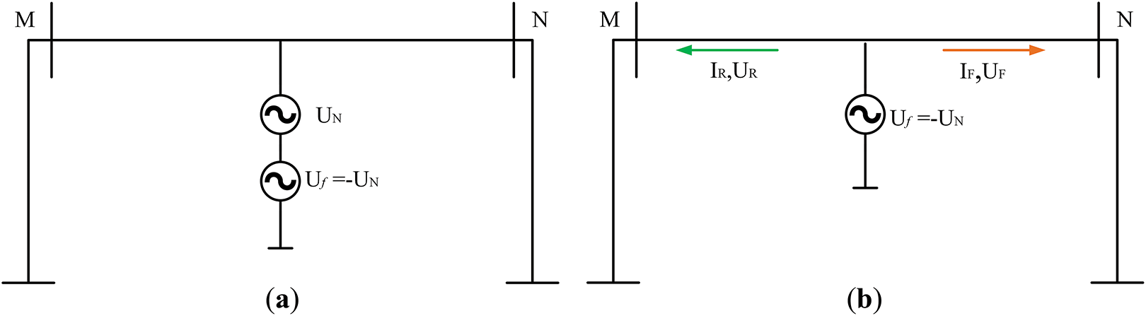
Figure 1: Fault network schematic. (a) Fault Equivalence Model; (b) fault-induced component
TWs have directionality. Based on the direction in which the bus is pointing toward the load, TW can be categorized into forward TW and reverse TW, according to the principle of TW propagation can be seen in Fig. 1 of the forward voltage TW
Fig. 2 shows a typical secondary radiation multi-segmented overhead line wiring pattern. Assuming the direction of bus-to-load is positive, the line impedance is
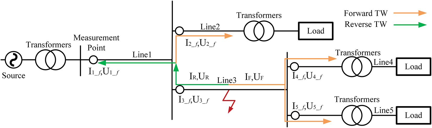
Figure 2: Secondary radial multi-segmented overhead lines
The reverse TW flow of Line 3 is transmitted through the secondary bus to Line 2, and the forward TW flow is transmitted through the tertiary bus to Lines 4 and 5, propagating toward loads along the normal power flow direction. For Lines 4 and 5, the fault-induced voltage and current at the head of their respective line are shown as Eq. (3):
For Line 2, the fault-induced voltage and current at the head of the line are shown as Eq. (4):
The preceding analysis demonstrates that at the moment of line fault, the voltage and current measured at the head of the fault line and its upstream line have the opposite polarity of the TW. In contrast, the voltage and current TWs measured at the head of the fault line and its downstream line or parallel line have the same polarity.
The above theory is based on a single conductor for elaboration, while the actual distribution line is three-phase circuits. When the fault occurs, the measured TW signals
Due to conductor inductance, electromagnetic coupling exists between the three phases. Therefore, before analyzing the voltage and current TW signals, the electromagnetic coupling inherent in three-phase systems typically necessitates the application of phase-mode transformation theory for effective decoupling [20]. The Karrenbauer transformation matrix is the most widely used phase-mode transformation matrix, which is expressed in the form of the transformation matrices as Eq. (6):
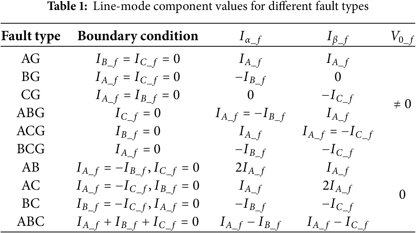
As can be seen from Eq. (6), the α line-mode component obtained after the Karrenbauer transform does not contain C-phase information. It cannot detect the single-phase-to-ground fault in phase C, and the β line-mode component does not contain B-phase information and cannot detect the single-phase-to-ground fault in phase B. Therefore, the fault-induced current and voltage TW signals undergo Karrenbauer phase-mode transformation to extract the mode maxima of the α and β line-mode components and calculate their products as shown in Eq. (7):
In Eq. (7):
The fault line discrimination vector is established based on the positive and negative values of each mode’s maximum value obtained, as shown in Eq. (8):
In Eq. (8): When
When the line occurs the single-phase-to-ground fault on phase C, the elements in
From the above analysis, the fault line discrimination process can be obtained:
I. Obtain the TW signals of current and voltage from the TW measuring instrument at the head of each line and calculate the fault-induced component;
II. Decouple the α and β line-mode components of the fault-induced current and voltage TWs using the Karrenbauer transform;
III. Extract the mode maxima of the α and β line-mode components of the fault-induced current and voltage TWs and calculate their products to construct the fault line discrimination vector
IV. Select the fault line discrimination vector whose elements are all non-zero. The fault line number corresponds to the index of the last element where the value equals −1.
Identifying the fault type and fault phase can assist maintenance teams in implementing targeted repair strategies. When the system experiences a ground fault, system symmetry is disrupted, resulting in significant changes in the three-phase voltage and current distributions, which in turn generates the zero sequence component that is crucial for ground fault detection. However, in the ungrounded neutral system, there is no zero-sequence current physical path, and when a ground fault occurs in the system, although the line capacitance to ground can provide a small capacitive current, the overhead line capacitance to ground is small, the capacitive current amplitude is low, it is not enough to form an effective zero-sequence current. Therefore, this article uses the zero-sequence voltage
Under different fault types,
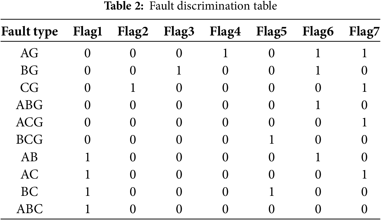
For the relationship between the values of
Flag1:
Flag5:
When each Flag condition is established, the Flag value is set to 1. According to the value of Flag1–Flag7, the Fault discrimination table can be obtained as Table 2:
Upon fault occurrence, computation of all fault discrimination marks is performed, and fault type is determined through Table 2.
3 Double-Ended TW Ranging Formula with the Effect of Wave Velocity Removed
3.1 Conventional Double-Ended TW Ranging Formula
When a fault occurs on a transmission line, the additional potential at the fault point will excite a transient TW and propagate along the fault line, exhibiting both refractive and reflective phenomena at wave impedance discontinuity interfaces. The double-ended TW method exploits the temporal relationship between wave propagation delays and transmission path lengths to determine the fault position. The fault-induced TW propagation characteristics through the line conductors are depicted in Fig. 3:
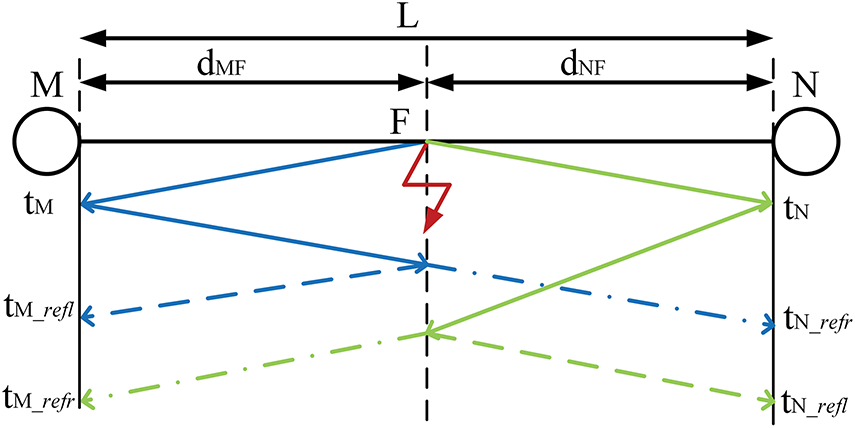
Figure 3: Faulty TW propagation path
In Fig. 3,
In Eq. (9):
As can be seen from Eq. (9), the accuracy of FL results depends on the arrival time of the TWs at measurement terminals and wave velocity. In engineering practice,
3.2 Improved Double-Ended TW Ranging Formula
To eliminate the effects of wave velocity uncertainty on the FL results, this study develops a reflection-based double-ended TW ranging method that overcomes the sensitivity of ranging results to wave velocity.
Assuming that
When
Similarly, when
From the above equation, it can be seen that the FL results are only related to the time of the first TW wave head and the first reflected wave head at the measurement end, successfully eliminating the inherent effect of wave velocity uncertainty on the ranging results.
4 FL Method Based on MODWT Combined with Improved TEO
In addition to the wave velocity, the time calibration accuracy of the fault TW arriving at the measurement end also directly affects the FL results; the improved double-ended TW ranging formula based on the TW reflection principle needs to measure the reflected wave head moment, the TW will be attenuated during propagation due to the loss of the line, the energy dispersion in the refraction and reflection will lead to difficulties in the calibration of the reflected wave head. Therefore, to enhance the precision of wave head identification, this study proposes a novel detection algorithm that integrates the MODWT with an improved TEO approach.
MODWT is a redundant wavelet transform method that eliminates the down-sampling operation in the DWT and utilizes the maximum overlap decomposition strategy; the coefficient length of each layer of decomposition is consistent with the length of the original signal, it can preserve complete time-frequency characteristics while preventing high-frequency component loss caused by down-sampling, and the MODWT can deal with signals of arbitrary length, and in practical engineering, we often encounter signals that are not a power of two, and MODWT does not need to make up the zero or truncate the signal, which reduces human interference [22]. MODWT has better time-frequency localization characteristics compared to the discrete wavelet transform, allowing it to capture local signal features more effectively and align with the requirements of high-precision, noise-resistant, and robust feature extraction for the study of FL of power distribution lines.
For any sampling length
As shown in Eq. (15), energy normalization of the up-sampled extended filter ensures that the total energy of each layer of the filter is the same as that of the original filter, thus satisfying the energy conservation condition:
In Eq. (15):
A filtering operation without down-sampling is performed on the signal to obtain the detail coefficients
In Eq. (16):
The TEO is a nonlinear signal processing technique that can instantaneously detect both energy and frequency variations using merely three consecutive signal samples, with a simple computational implementation and low computational complexity [23]. For a discrete signal
By introducing the sum of squares of the product terms, the estimation of signal energy can be enhanced with stronger noise immunity, better time domain resolution, and more accurate energy estimation in detecting signal mutation points. For a discrete signal
In Eq. (18):
When a line fault occurs, a high-frequency transient TW is generated at the fault point; the first layer of detail coefficients
4.3 Multi-Branch Line FL Process
The proposed multi-branch distribution line FL method based on MODWT combined with improved TEO is shown in Fig. 4. The implementation procedure consists of five key steps:
I. When a fault occurs on the line, extract the fault current and voltage TW by the TW measurement instrument at both ends of each line.
II. Following the method in Section 2.1, calculate the fault-induced current and voltage signals of each line, decouple them using the Karrenbauer transformation, calculate the modal maximum value of the line-mode component of the fault-induced signal at the head of each line, construct a fault line discrimination vector, and determine the fault line.
III. Following the method in Section 2.2, calculate the fault-induced line-mode current
IV. When a single-phase-to-ground fault on phase C occurs in a line, perform MODWT decomposition of the β line-mode voltage at both ends of the fault line; when other faults occur, perform MODWT decomposition of the α line-mode voltage at both ends of the fault line, calculate the energy spectrum of the first layer of detail coefficients
V. Using the improved double-ended TW ranging formula based on the TW reflection principle, the wave head time calibrated by step IV is brought into Eqs. (12) and (13) to calculate the fault distance.
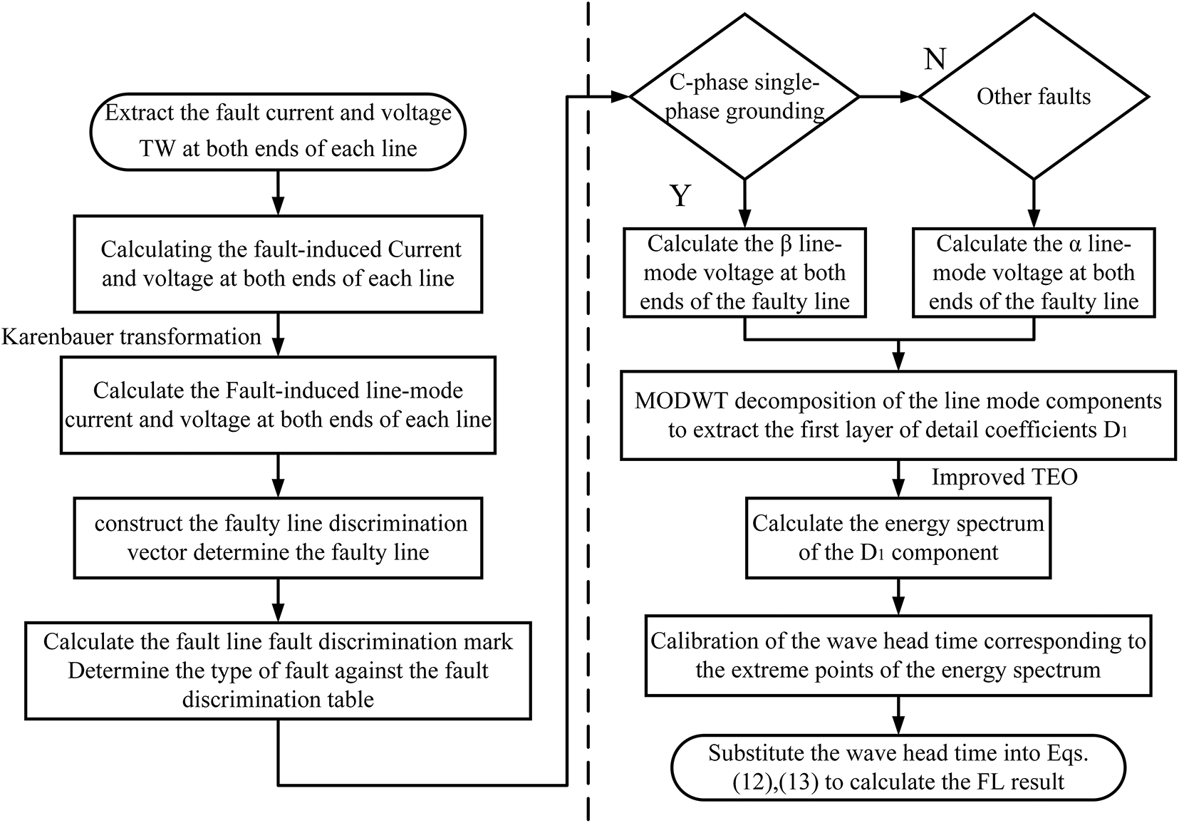
Figure 4: Multi-branch FL process
In the Matlab/Simulink platform, a 10 kV ungrounded neutral system distribution line fault model was built, as shown in Fig. 5.
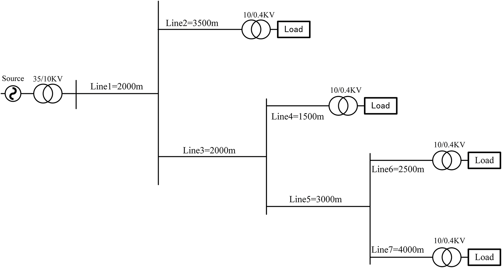
Figure 5: Topology of a single-ended radial distribution network for the ungrounded neutral system
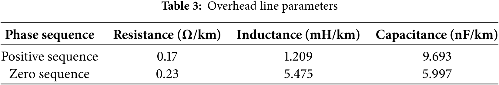
The source-side transformer is a Yd11-connection, and the load-side transformer is a Dyn11-connection. The load is a delta-connected constant-impedance load, whose active power is 0.08 MVA, reactive power is 0.06 MVA, overhead line parameters are set as shown in Table 3, and the related parameters meet the requirements of actual engineering parameters of a 10 kV distribution network. The simulation duration is 0.06 s, and the sampling frequency is 10 MHz.
Using the three-phase line fault module to set up a single-phase-to-ground fault on phase A with a grounding resistance of 5 Ω and a fault initial phase angle of 30° in Line 5, the length of Line 5 is 3 km, and the fault point is 1.4 km from the head of Line 5. The changes in fault current and voltage line-mode components at the head of each line during the fault transient are shown in Figs. 6 and 7:
From Figs. 6 and 7, it can be seen that the polarity of the line-mode voltage and current TW mutation amount of Lines 1, 3, and 5 is opposite, and the polarity of the line-mode voltage and current TW mutation amount of Lines 2, 4, 6, and 7 is the same. Through the analysis in Section 2, it can be concluded that the fault line discrimination vector
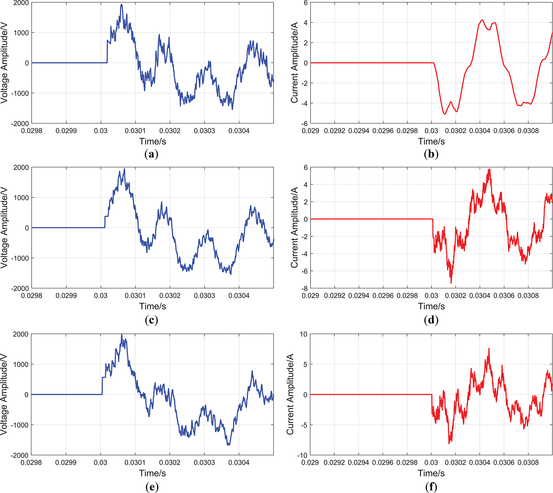
Figure 6: Fault-induced line mode at the head of the fault line and its upstream line. (a) Fault-induced line-mode voltage at the head of Line 1; (b) fault-induced line-mode current at the head of Line 1; (c) fault-induced line-mode voltage at the head of Line 3; (d) fault-induced line-mode current at the head of Line 3; (e) fault-induced line-mode voltage at the head of Line 5; (f) fault-induced line-mode current at the head of Line 5
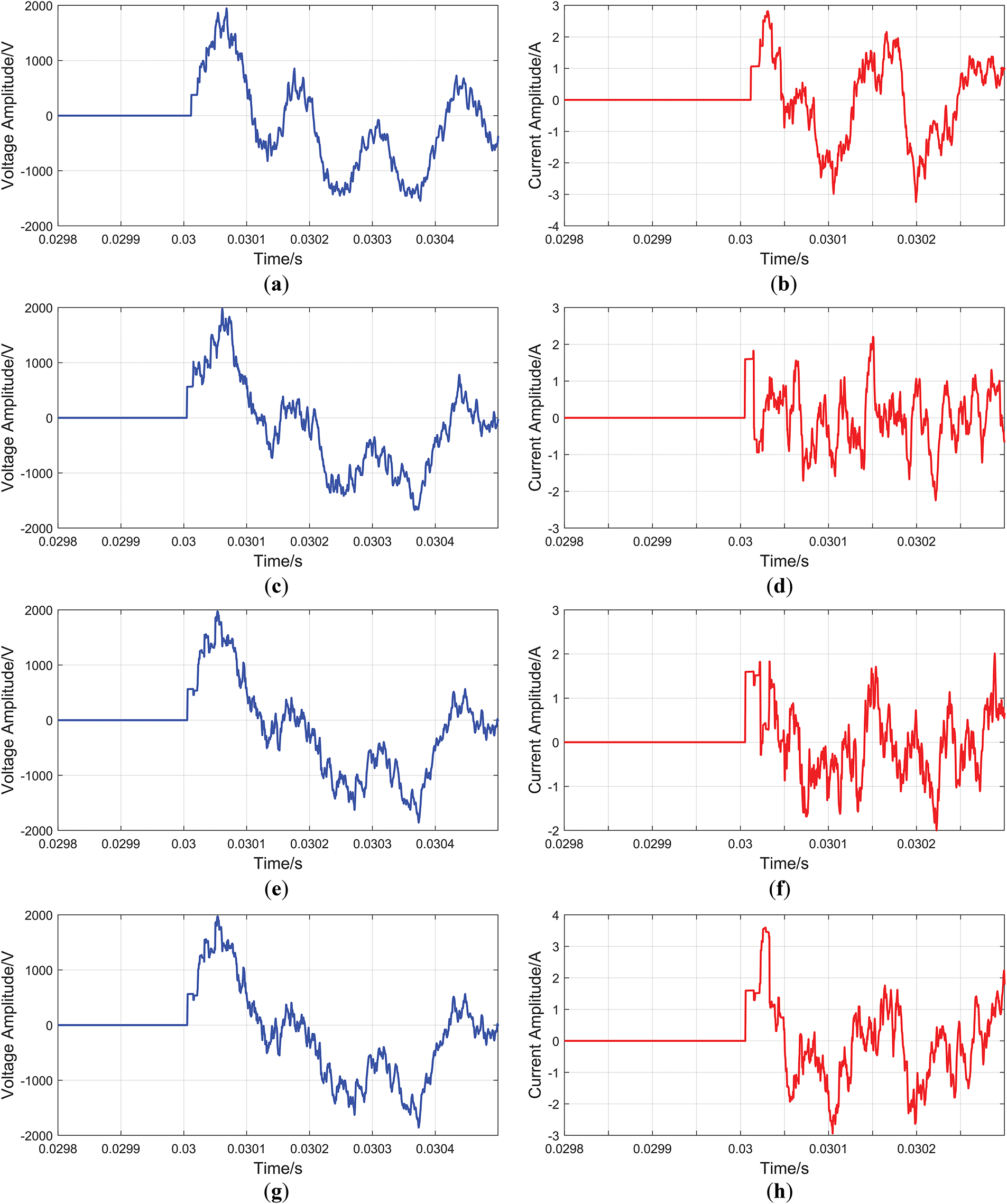
Figure 7: Fault-induced line-mode at the head of Lines downstream and parallel lines of the fault line. (a) Fault-induced line-mode voltage at the head of Line 2; (b) fault-induced line-mode current at the head of Line 2; (c) fault-induced line-mode voltage at the head of Line 4; (d) fault-induced line-mode current at the head of Line 4; (e) fault-induced line-mode voltage at the head of Line 6; (f) fault-induced line-mode current at the head of Line 6; (g) fault-induced line-mode voltage at the head of Line 7; (h) fault-induced line-mode current at the head of Line 7
The α line-mode voltage at both ends of Line 5 is extracted for MODWT decomposition, and the selected wavelet base is the db4 wavelet, which is decomposed into four layers to extract the
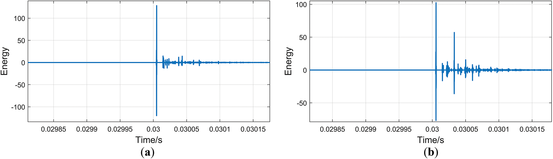
Figure 8:
The energy spectrum of the
From Fig. 9a,b, it can be seen that the initial wave head arrives at the two ends of the fault line at 30.0048 ms and 30.0055 ms, respectively. From Fig. 9c,d, it can be seen that the time of the second wave head detected by the measuring instrument at the two ends is 30.0144 and 30.0151 ms, respectively. By using Eq. (12), the calculated FL result is determined to be 1398.058 m from the line terminal, with a mere 1.942 m positioning deviation. This article introduces the relative error
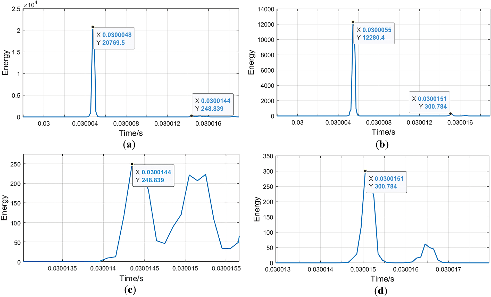
Figure 9:
In Eq. (19):
According to Eq. (19), the relative error is only 0.06%, which proves the accuracy of the method proposed in this paper.
5.2 Effect of Fault Conditions on Fault Discrimination and Location Results
Different fault conditions will affect the amplitude and slope of TWs to varying degrees, leading to a reduction in wave head extraction accuracy and thus increase the FL result error. In order to prove the robustness of the proposed method in different fault scenarios, the following comparison experiments are conducted:
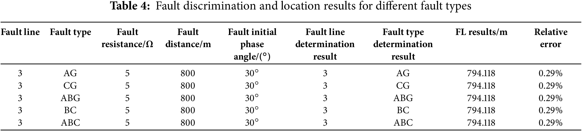
Setting the fault line as Line 3 with a fault resistance of 5 Ω and a fault initial phase angle of 30°. Different types of faults occur at 800 m from the head of the line. The FL results shown in Table 4 indicate that the fault types do not affect the FL results of the method proposed in this paper.
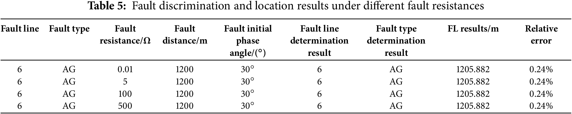
Set the fault line as Line 6 with a fault initial phase angle of 30° and the single-phase-to-ground fault on phase A at 1200 m from the head of the line. Different fault resistances are set to simulate metallic short-circuit faults, low-resistance short-circuit faults, and high-resistance short-circuit faults. The results of FL shown in Table 5 indicate that the fault resistances do not affect the FL results of the method proposed in this paper.
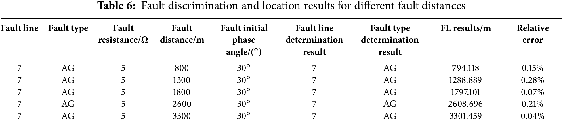
Set the fault line as Line 7 with a fault resistance of 5 Ω and a fault initial phase angle of 30°, and set the single-phase-to-ground fault on phase A with different fault distances. The FL results shown in Table 6 indicate that the fault distance has little impact on the FL results of the method proposed in this paper.
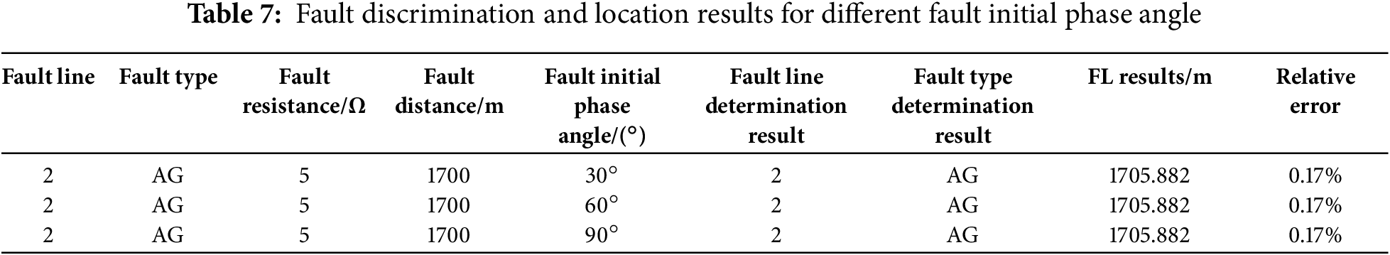
Set the fault line as Line 2 with a fault resistance of 5 Ω, and a single-phase-to-ground fault on phase A occurs at 1700 m from the head of the line. Set the initial phase angle of the fault to 30°, 60°, and 90°, respectively. The FL results shown in Table 7 indicate that the fault initial phase angles do not affect the FL results of the method proposed in this paper.
5.3 Comparison of FL Results of Different Methods
To further demonstrate that the method proposed in this paper is more effective than the commonly used methods, this subsection compares the method of this paper with other conventional methods in a comparative experiment. Set a single-phase-to-ground fault on phase A with a fault resistance of 5 Ω and a fault initial phase angle of 30° in Line 1, and detect the fault distance through four different methods. Based on the parameters of the line model in this article, use Eq. (10) to calculate the wave velocity value
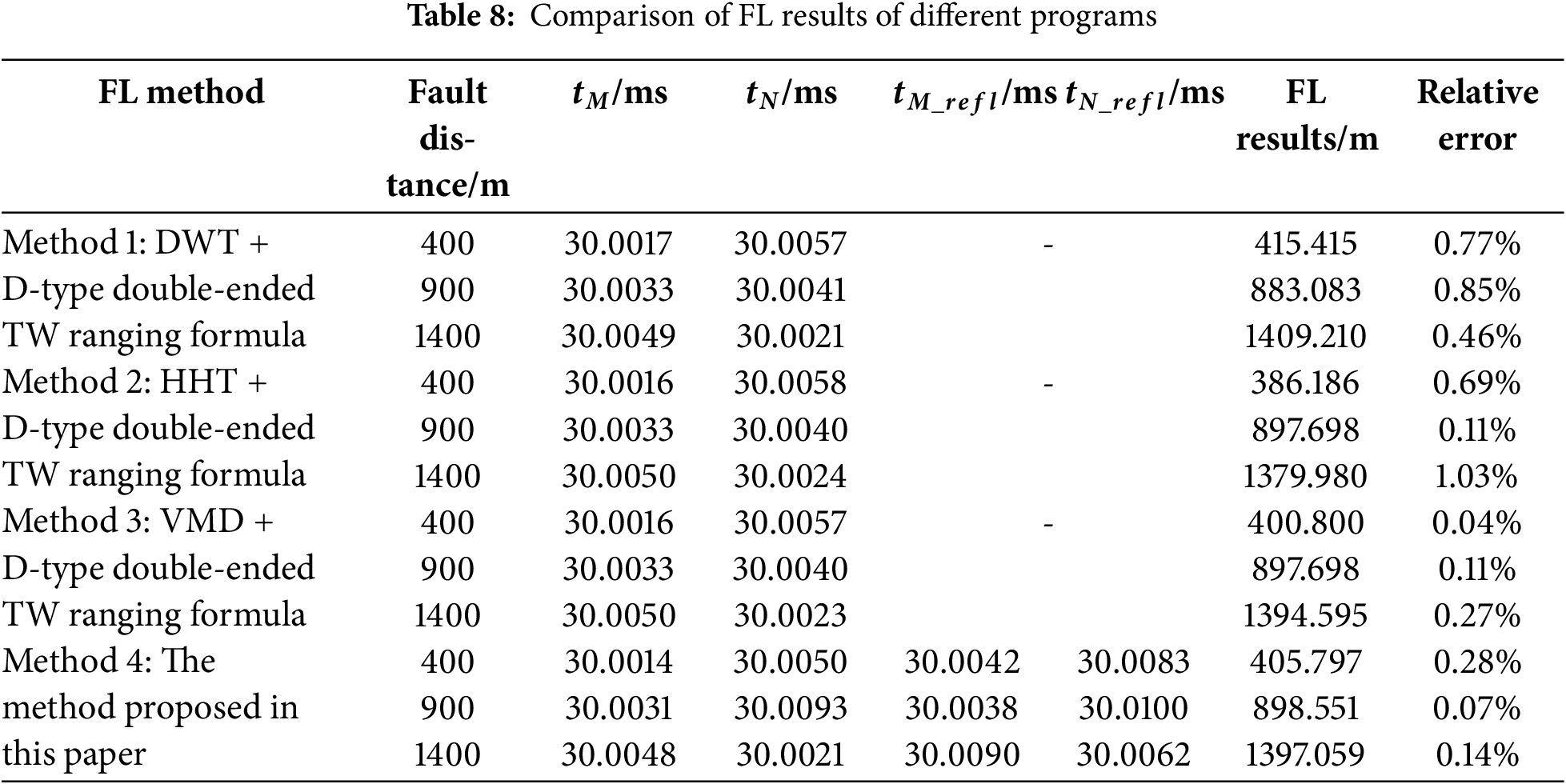
According to Table 8, the proposed methodology achieves significantly higher ranging accuracy compared to the combination of DWT and EMD with the D-type double-ended TW ranging formula. The ranging accuracy of VMD combined with the D-type double-ended TW ranging formula shows comparable accuracy to the method proposed in this paper; however, VMD has higher computational complexity and longer solving times. Consequently, the proposed methodology demonstrates superior accuracy and computational efficiency, rendering it particularly suitable for practical engineering applications.
5.4 Validation of the Effectiveness of Module Improvements
To demonstrate the effectiveness of the improvements of the components proposed in this paper, the following four schemes are proposed: Method 1: MODWT with the D-type double-ended TW ranging formula; Method 2: MODWT combined with TEO and the improved double-ended TW ranging formula; Method 3: the method proposed in this paper. The single-phase-to-ground fault on phase A with a grounding resistance of 5 Ω and a fault initial phase angle of 30° is set in Line 4, and the FL results are shown in Table 9.
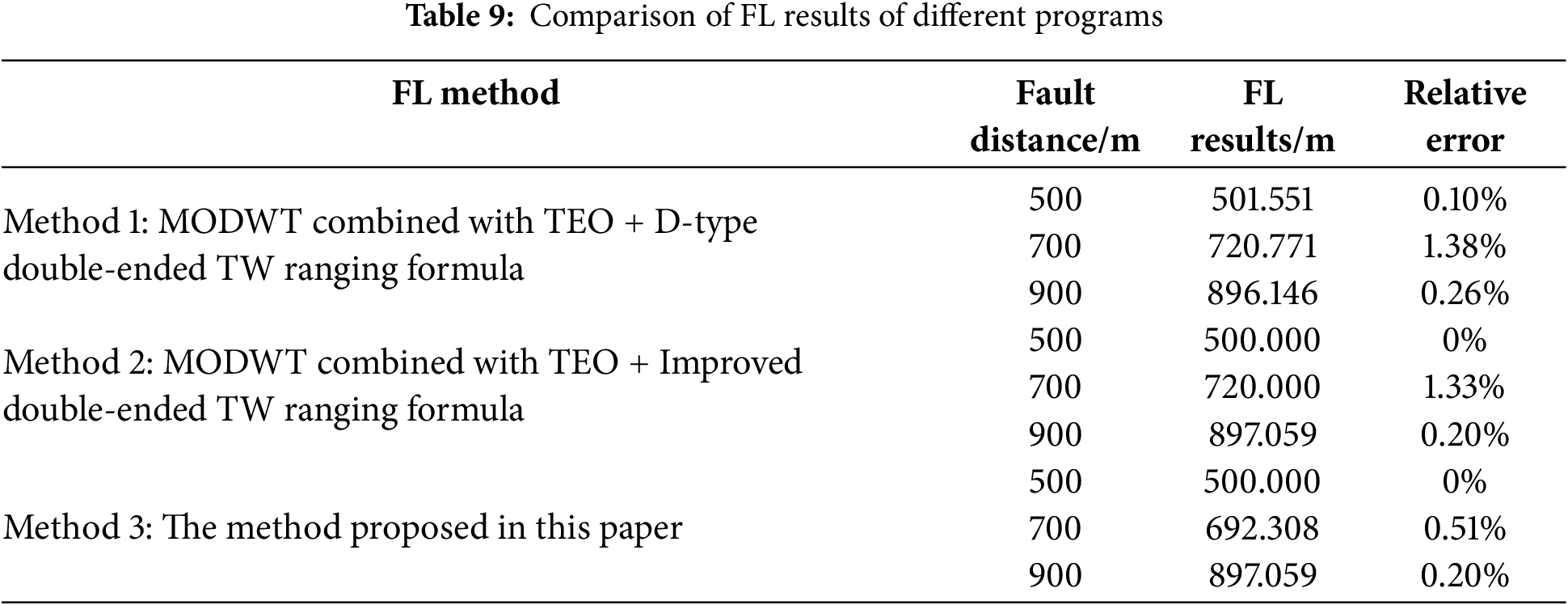
According to Table 9, the proposed methodology demonstrates enhanced measurement precision compared to both Method 1 and Method 2 approaches, proving that the improvement of the TEO energy operator in this paper can better extract the high-frequency characteristics of fault TW and the improved double-ended TW formula can effectively eliminate the inherent error caused by wave velocity uncertainty on the FL results.
This article proposes a distribution line FL method that considers the topology of the distribution network to address the difficulties in distinguishing fault branches, the need to improve the accuracy of commonly used signal decomposition algorithms in extracting TW wave heads, and the interference of uncertain wave velocity values on distance measurement results. Based on rigorous theoretical analysis and comprehensive simulation experiments, the key conclusions are summarized as follows:
(1) A fault line determination method based on the polarity of fault-induced current and voltage TW mutation amount and a fault type discrimination mechanism combining the line-mode component of fault-induced current and zero-sequence voltage are proposed, which can quickly and accurately determine the fault line and the fault type, without being affected by the topology and operation mode of the distribution network, provide a basis for the modulus selection during FL and fault repair work.
(2) The proposed wave head detection algorithm is based on the combination of MODWT with improved TEO, which utilizes MODWT without the down-sampling operation to better capture the time-frequency local features of the signal and introduces the sum-of-squares term to enhance the feature extraction capability and anti-interference ability of TEO. This combined approach offers the advantages of small computation and high accuracy, enabling the precise identification of both the first and reflected TW arrival times.
(3) An improved double-ended TW ranging formula based on the TW reflection principle is proposed, which utilizes the time difference between the first wave head and the first reflecting wave head to successfully eliminate the effect of wave velocity uncertainty on the FL results. Combined with the wave head detection algorithm proposed in this paper, the FL accuracy is controlled within 0.5%, and the FL results are not affected by the fault type, fault resistance, fault distance, and fault initial phase angle, which can be well applied in engineering practice.
It should be emphasized that time synchronization has no effect on the fault line determination result and fault type determination result, but it affects the accuracy of the fault location results. Future work will focus on eliminating the effect of time synchronization on the FL results.
Acknowledgement: Not applicable.
Funding Statement: This work was funded by the project of Guizhou Power Grid Co., Ltd. Guiyang Power Supply Bureau (No. GZKJXM20232317).
Author Contributions: The authors confirm their contribution to the paper as follows: The study conception and design: Pan Duan, Enze Peng; data collection: Pan Duan, Enze Peng; analysis and interpretation of results: Pan Duan, Enze Peng; draft manuscript preparation: Pan Duan, Enze Peng. All authors reviewed the results and approved the final version of the manuscript.
Availability of Data and Materials: The authors confirm that the data supporting the findings of this study are available within the article.
Ethics Approval: Not applicable.
Conflicts of Interest: The authors declare no conflicts of interest to report regarding the present study.
Abbreviations
| FL | Fault Location |
| MODWT | Maximal Overlap Discrete Wavelet Transform |
| TEO | Teager Energy Operator |
| TW | Traveling Wave |
| DWT | Discrete Wavelet Transform |
| HHT | Hilbert-Huang Transform |
| VMD | Variable Mode Decomposition |
| Nomenclature | |
| Forward voltage/current | |
| Reverse voltage/current | |
| Measured voltage/current in phase | |
| Pre-fault voltage/current in phase | |
| Fault-induced voltage/current in phase | |
| α-, β-, and zero-mode currents | |
| Zero-mode voltage | |
| Products of α and β line-mode voltage and current modal extrema for line | |
| Sign indicators for | |
| Total length of line | |
| Fault distance to M/N end | |
| First arrival time of traveling wave at M/N end | |
| Time of traveling wave arrival at M/N end after first reflection | |
| Time of traveling wave arrival at M/N end after first refraction | |
| The weight coefficient of the sum of squares of the product terms | |
| Time of failure | |
| Wave velocity | |
| Impedance of line | |
| Inductance of line | |
| Capacitance of line | |
| The | |
| The | |
| The | |
| The | |
| The | |
| The | |
References
1. Dashti R, Ghasemi M, Daisy M. Fault location in power distribution network with presence of distributed gener-ation resources using impedance based method and applying π line model. Energy. 2018;159(1):344–60. doi:10.1016/j.energy.2018.06.111. [Google Scholar] [CrossRef]
2. Mirshekali H, Dashti R, Keshavarz A, Shaker HR. Machine learning-based fault location for smart distribution networks equipped with micro-PMU. Sensors. 2022;22(3):945. doi:10.3390/s22030945. [Google Scholar] [PubMed] [CrossRef]
3. Chen X, Zhu YL, Zhao XS, Zhao L, Guo X. Traveling wave fault location for T-shaped transmission line considering change of line length. Power Syst Technol. 2015;39(5):1438–43. doi:10.13335/j.1000-3673.pst.2015.05.040. [Google Scholar] [CrossRef]
4. Teng JH, Huang WH, Luan SW. Automatic and fast faulted line-section location method for distribution systems based on fault indicators. IEEE Trans Power Syst. 2014;29(4):1653–62. doi:10.1109/TPWRS.2013.2294338. [Google Scholar] [CrossRef]
5. Boem F, Gallo AJ, Raimondo DM, Parisini T. Distributed fault-tolerant control of large-scale systems: an active fault diagnosis approach. IEEE Trans Control Netw Syst. 2019;7(1):288–301. doi:10.1109/TCNS.2019.2913557. [Google Scholar] [CrossRef]
6. Wang Q, Jin T, Mohamed MA. A fast and robust fault section location method for power distribution systems considering multisource information. IEEE Syst J. 2021;16(2):1954–64. doi:10.1109/JSYST.2021.3057663. [Google Scholar] [CrossRef]
7. Wang Q, Xiao Y, Dampage U, Alkuhayli A, Alhelou HH, Annuk A, et al. An effective fault section location method based three-line defense scheme considering distribution systems resilience. Energy Rep. 2022;8(2):10937–49. doi:10.1016/j.egyr.2022.08.235. [Google Scholar] [CrossRef]
8. De La Cruz J, Gómez-Luna E, Ali M, Vasquez JC, Guerrero JM. Fault location for distribution smart grids: literature overview, challenges, solutions, and future trends. Energies. 2023;16(5):2280. doi:10.3390/en16052280. [Google Scholar] [CrossRef]
9. Xie L, Wang Y, Xiao Y, Zeng X, Mo Y, Long Z. Fault location method for multi-section hybrid lines considering velocity uncertainty. Int J Electr Power Energy Syst. 2025;164(4):110405. doi:10.1016/j.ijepes.2024.110405. [Google Scholar] [CrossRef]
10. Xie L, Luo L, Ma J, Li Y, Zhang M, Zeng X, et al. A novel fault location method for hybrid lines based on traveling wave. Int J Electr Power Energy Syst. 2022;141(4):108102. doi:10.1016/j.ijepes.2022.108102. [Google Scholar] [CrossRef]
11. Leng H, He S, Qiu J, Liu F, Huang X, Liu F, et al. Multi-branch fault line location method based on time difference matrix fitting. Energy Eng. 2024;121(1):77–94. doi:10.32604/ee.2023.028340. [Google Scholar] [CrossRef]
12. Li C, Liu G, Yu C, Wang C, Chen F, Wan S. A traveling wave based fault location method for high-voltage transmission lines. J Electr Power Sci Technol. 2023;38(2):179–85. doi:10.19781/j.issn.1673-9140.2023.02.020. [Google Scholar] [CrossRef]
13. Fayazi M, Joorabian M, Saffarian A, Monadi M. A single-ended traveling wave based fault location method using DWT in hybrid parallel HVAC/HVDC overhead transmission lines on the same tower. Electr Power Syst Res. 2023;220(1):109302. doi:10.1016/j.epsr.2023.109302. [Google Scholar] [CrossRef]
14. Cao W, Zhao L, Li Z, Chen J, Xu M, Niu R. Fault location study of overhead line-cable lines with branches. Processes. 2023;11(8):2381. doi:10.3390/pr11082381. [Google Scholar] [CrossRef]
15. Wu J, Lan S, Xiao S, Yuan YB. A single pole-to-ground fault location system for MMC-HVDC transmission lines based on active pulse and CEEMDAN. IEEE Access. 2021;9:42226–35. doi:10.1109/ACCESS.2021.3062703. [Google Scholar] [CrossRef]
16. Yu K, Zhu X, Cao W. Study on traveling wave fault localization of transmission line based on NGO-VMD algorithm. Energies. 2024;17(9):2003. doi:10.3390/en17092003. [Google Scholar] [CrossRef]
17. Dardengo VP, Fardin JF, de Almeida MC. Single-terminal fault location in HVDC lines with accurate wave velocity estimation. Electr Power Syst Res. 2021;194(13):107057. doi:10.1016/j.epsr.2021.107057. [Google Scholar] [CrossRef]
18. Yang Y, Zhang Q, Wang M, Wang X, Qi E. Fault location method of multi-terminal transmission line based on fault branch judgment matrix. Appl Sci. 2023;13(2):1174. doi:10.3390/app13021174. [Google Scholar] [CrossRef]
19. Zhou J, Qu Z, Zhan Z. A CPO-VMD based traveling wave fault location method for transmission lines. J Electr Power Sci Technol. 2024;1–11. [cited 2025 Jun 19]. Available from: http://kns.cnki.net/kcms/detail/43.1475.TM.20241120.1100.002.html. [Google Scholar]
20. Tang M, Lu H, Li B. Fault location of untransposed double-circuit transmission lines based on an improved Karrenbauer matrix and the QPSO algorithm. Prot Control Mod Power Syst. 2023;8(1):44. doi:10.1186/s41601-023-00318-6. [Google Scholar] [CrossRef]
21. Mao X, Xiang B, Tu S. Research on power penetration cable line fault location based on distributed traveling wave location technology. AIP Adv. 2022;12(5):055024. doi:10.1063/5.0093049. [Google Scholar] [CrossRef]
22. Zhang T, Han K, Li H, Liu S, Chen F. Two terminals protection method for HVDC transmission lines based on maximal overlap discrete wavelet transform and cross-correlation coefficient of traveling wave. Energy Rep. 2023;9(3):1133–48. doi:10.1016/j.egyr.2023.04.134. [Google Scholar] [CrossRef]
23. Cao W, Zhang F, Chen X, Zhang B, Li J, Xu M. A study on fault localization method of three-terminal multi-section overhead line-cable hybrid line using MEEMD combined with teager energy operator algorithm. Processes. 2024;12(7):1360. doi:10.3390/pr12071360. [Google Scholar] [CrossRef]
Cite This Article
 Copyright © 2025 The Author(s). Published by Tech Science Press.
This work is licensed under a Creative Commons Attribution 4.0 International License , which permits unrestricted use, distribution, and reproduction in any medium, provided the original work is properly cited.
 Downloads
 Citation Tools