
 Submit a Paper
 Propose a Special lssue
 Open Access
ARTICLE
Virtual Synchronous Generator Control Strategy Based on Parameter Self-Tuning
1 School of Automation, Nanjing University of Information Science and Technology, Nanjing, 210044, China
2 School of Automation, Wuxi University, Wuxi, 214105, China
3 State Grid Beijing Electric Power Research Institute, Beijing, 100075, China
* Corresponding Author: Jin Lin. Email:
(This article belongs to the Special Issue: Innovations and Challenges in Smart Grid Technologies)
Energy Engineering 2026, 123(1), 8 https://doi.org/10.32604/ee.2025.069310
Received 20 June 2025; Accepted 14 August 2025; Issue published 27 December 2025
 View Full Text
 Download PDF
Abstract
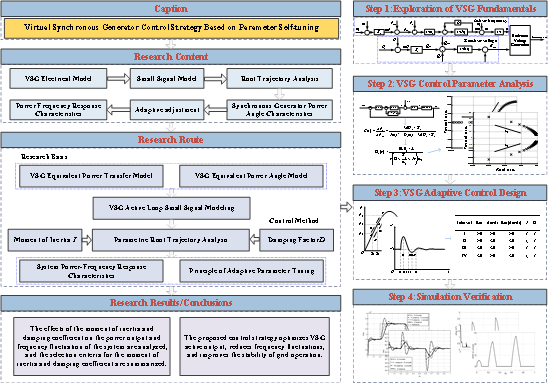
With the increasing integration of renewable energy, microgrids are increasingly facing stability challenges, primarily due to the lack of inherent inertia in inverter-dominated systems, which is traditionally provided by synchronous generators. To address this critical issue, Virtual Synchronous Generator (VSG) technology has emerged as a highly promising solution by emulating the inertia and damping characteristics of conventional synchronous generators. To enhance the operational efficiency of virtual synchronous generators (VSGs), this study employs small-signal modeling analysis, root locus methods, and synchronous generator power-angle characteristic analysis to comprehensively evaluate how virtual inertia and damping coefficients affect frequency stability and power output during transient processes. Based on these analyses, an adaptive control strategy is proposed: increasing the virtual inertia when the rotor angular velocity undergoes rapid changes, while strengthening the damping coefficient when the speed deviation exceeds a certain threshold to suppress angular velocity oscillations. To validate the effectiveness of the proposed method, a grid-connected VSG simulation platform was developed in MATLAB/Simulink. Comparative simulations demonstrate that the proposed adaptive control strategy outperforms conventional VSG methods by significantly reducing grid frequency deviations and shortening active power response time during active power command changes and load disturbances. This approach enhances microgrid stability and dynamic performance, confirming its viability for renewable-dominant power systems. Future work should focus on experimental validation and real-world parameter optimization, while further exploring the strategy’s effectiveness in improving VSG low-voltage ride-through (LVRT) capability and power-sharing applications in multi-parallel configurations.Graphic Abstract
Keywords
The rapid expansion of wind, photovoltaic, and other renewable energy sources has posed new challenges to power system stability. A critical issue stems from the integration of these energy sources through power electronic interfaces, particularly inverters, which have significantly altered grid dynamics [1,2]. Unlike traditional synchronous generators, inverter-based systems exhibit low inertia and damping characteristics, resulting in diminished frequency and voltage regulation capabilities [3]. To address these challenges, the Virtual Synchronous Generator (VSG) control method has emerged as a promising solution. By emulating the rotational inertia, damping effect, and primary frequency regulation capabilities of synchronous generators, VSG allows inverters to mimic the operational characteristics of conventional power plants during grid-connected operation. Studies have demonstrated that this approach can effectively enhance system stability and regulation performance [4,5]. Furthermore, to improve inverter control flexibility under varying operating conditions, researchers have increasingly focused on developing adaptive VSG control strategies with variable virtual inertia and damping coefficients [6,7].
Recent studies have made significant progress in developing adaptive VSG control strategies. Several notable contributions have advanced the field: Through analyzing parameter variation effects on system response, Reference [8] demonstrated that maintaining optimal damping ratios was crucial for VSG dynamic performance enhancement. Reference [9] proposed virtual inertia integration to boost inverter robustness and stability, employing an adaptive algorithm that maintained power and frequency stability during operational variations. Furthermore, References [10,11] developed dynamic virtual inertia adjustment methods based on system operational deviations to optimize microgrid performance. Reference [12] divided the oscillatory process after system disturbance into four stages. Based on the characteristics of VSG power oscillation and power angle variation in each stage, it adaptively adjusted the virtual inertia and damping coefficients to reduce overshoot and settling time during frequency dynamic transients. However, the parameter adjustment method described in Reference [12] only responded to angular frequency deviation and did not consider the influence of angular frequency change rate. Building on these works, Reference [13] introduced an innovative modification by replacing the angular frequency derivative term with active power deviation, thereby reducing noise interference and improving transient response. Although these studies have optimized the power output characteristics of VSG. However, the contradiction between dynamic stability and fast response, as well as the conflicts in multi-objective optimization, remain unresolved challenges.
Further studies focus on the selection of control parameters and the optimization of control strategies. Reference [14] employed a bang-bang control algorithm to achieve adaptive adjustment of the VSG moment of inertia. However, this approach exhibits drawbacks such as parameter discretization and potential system instability. Moreover, it fails to account for the influence of the damping coefficient on the system. Reference [15] proposed a VSG control method based on the direct Lyapunov approach, while Reference [16] developed a fuzzy control-based VSG strategy. However, both methods suffered from limitations such as complicated design processes, difficulties in parameter adjustment and tuning, and insufficient adaptability to dynamic system characteristics. Additionally, regarding the fuzzy control methodology presented in Reference [16], both the fuzzy rules and membership functions are entirely determined by researchers’ experience. Different rule sets can lead to inconsistent control performance, making it difficult to achieve the theoretical optimum. Furthermore, fixed rules and membership functions cannot adapt to environmental variations caused by temperature and load fluctuations, nor accommodate system parameter drift resulting from device aging or sensor deviations. Reference [17] improved upon conventional adaptive VSG control by incorporating output speed feedback to adjust damping coefficients, which effectively suppressed power overshoot during dynamic regulation. Furthermore, it introduced adaptive adjustment of virtual inertia coefficients based on the rate of frequency change during transient processes. This approach not only reduced settling time but also narrowed the regulation range of virtual rotational inertia during system operation. Reference [18] achieved coordinated control of multiple parameters through relationship optimization, demonstrating superior frequency stabilization. For islanding conditions, Reference [19] developed an adaptive tuning strategy that improved frequency regulation under uncertainties in load and PV output.
In further research on VSG parameter adaptive control, with advances in machine learning methods, scholars have attempted to integrate these techniques into VSG control. Representative studies include: Reference [20] proposed a hybrid control strategy combining fuzzy control with model predictive control (MPC) to adaptively adjust VSG’s virtual inertia and damping coefficients. The study compared this combined approach against standalone fuzzy and MPC methods to validate its effectiveness. However, during adaptive regulation, the virtual inertia parameter abruptly transitioned to negative values, causing the virtual synchronous generator to exhibit negative-inertia behavior. Whether power electronic devices can operate with negative inertia in practical grid environments remains contentious. Reference [21] pioneered the application of radial basis function (RBF) neural networks to VSG control, leveraging their algorithmic simplicity, powerful learning capability, and rapid convergence to adjust virtual inertia in real-time. Under predetermined inertia values, the study introduced adaptive damping based on optimal damping ratio theory to further suppress power oscillations, comparing this improved strategy against linear control methods. Nevertheless, the control scheme in [21] suffers from excessive complexity and restrictive constraints that hinder practical implementation. Experimental results additionally revealed that during power imbalance and grid frequency fluctuations, the damping coefficient exhibited greater oscillation amplitudes than linear control approaches. These studies highlight both the progress in adaptive VSG control and the need to further investigate parameter-system dynamics relationships.
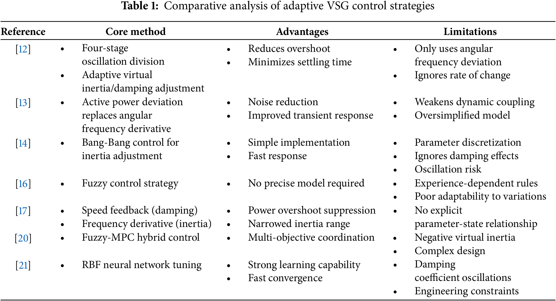
Drawing from the literature review section, we have summarized Table 1 to reflect the core methods and their advantages and disadvantages in current research.
Based on the identified limitations in existing adaptive VSG control strategies, such as the lack of explicit relationships between adaptive parameters and system states, inherent coordination difficulties in multi-parameter adjustment mechanisms, and insufficient mitigation of dynamic stability risks including damping oscillations and frequency deviations, this study aims to explore refined control approaches. We systematically analyze how key VSG parameters impact power output and system stability. Building on this foundation, virtual variables and control parameters are optimized through correlation with maximum system capacity configuration and allowable frequency deviation thresholds. Explicit parameter selection criteria are subsequently established to maximize adaptive control effectiveness. Specifically, the study first constructs a small-signal model of the VSG active power loop to meticulously examine how virtual inertia and damping coefficients influence frequency fluctuations and active power output dynamics during transient conditions. In additional, a mathematical relationship is established between angular frequency variations (including their offsets) and these adaptive parameters. Based on these findings, precise selection criteria for control parameters are formulated, where inertia and damping values are dynamically adjusted according to real-time system behavior. Moreover, by optimizing the control parameters, this study also effectively mitigates the over-regulation of virtual inertia in the adaptive adjustment process. For validation, a comprehensive grid-connected VSG simulation model was developed in MATLAB/Simulink. Three operational scenarios—active power command variation, load change, and grid voltage sag—are designed. Comparative analyses of dynamic response curves for both system frequency and active power output across various control methods demonstrate the proposed approach’s superior performance.
VSG technology plays a pivotal role in improving power system stability by emulating the inertial and damping properties of traditional synchronous generators. As depicted in Fig. 1, the primary circuit topology and control architecture of the VSG are illustrated.
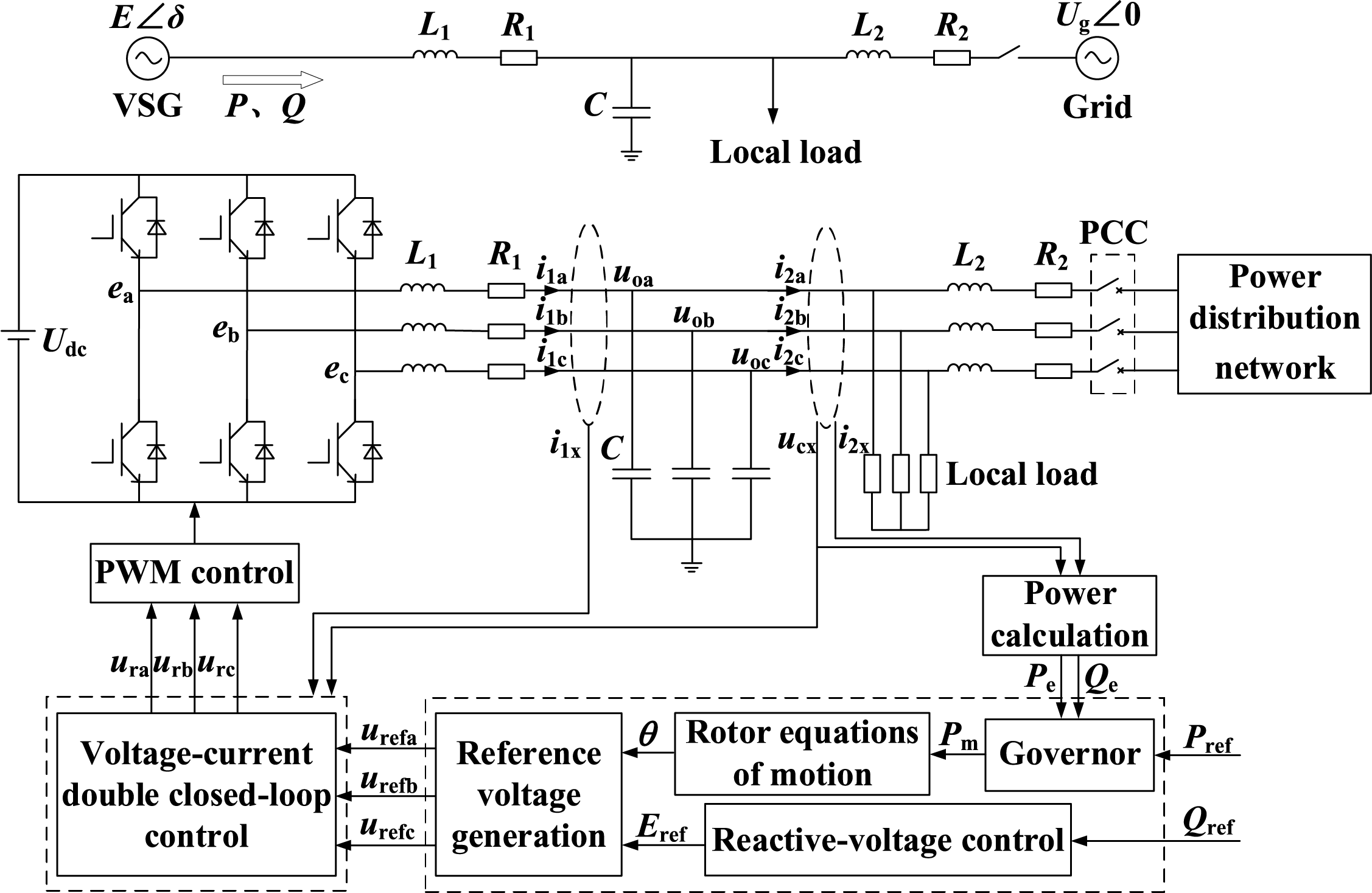
Figure 1: VSG structure
The diagram can be divided into three main components. First, the main power circuit employs a three-phase bridge inverter configuration, which generates three-phase sinusoidal voltage through an LC filter circuit and can operate in both standalone and grid-connected modes. Second, the VSG power loop serves as the core of the virtual synchronous generator, comprising both active power-frequency control and reactive power-voltage control. Notably, the active power-frequency control incorporates equations for both the rotor motion and the governor dynamics. Third, the dual-loop voltage and current control section completes the system architecture. The core objective of this control strategy is to enable the inverter to mimic the operational dynamics of a synchronous generator, thereby providing analogous functional attributes. To systematically evaluate the VSG’s control performance in mitigating frequency instability and power fluctuations caused by renewable generation variability, this study initially adopts an ideal DC voltage source assumption. While this simplification allows for focused analysis of the control dynamics under standardized conditions, it should be noted that practical implementations require additional energy storage devices to suppress DC-side voltage fluctuations, particularly in high-penetration scenarios [22,23].
In the schematic diagram, Ug represents the grid phase voltage, with its phase angle fixed at 0°. The inverter generates a phase voltage denoted as E, characterized by a phase angle δ. Udc symbolizes the DC-link voltage. On the inverter side, L1, R1, and C correspond to the inductance, resistance, and capacitance of the filter components, respectively. Similarly, L2 and R2 represent the impedance on the grid side. The voltages at the midpoint of each inverter bridge arm are labeled as ea, eb, and ec. The three-phase inductor currents are indicated by i1x (x = a, b, c), while the port voltages are denoted as uox (x = a, b, c). The three-phase currents injected into the load and grid after filtering are represented by i2x (x = a, b, c), and the three-phase capacitor voltages are expressed as ucx (x = a, b, c). The active power reference value is designated as Pref, and the real-time active power output of the inverter is Pe. Similarly, the reactive power reference value is Qref, and the real-time reactive power output is Qe. The VSG power control loop generates a reference voltage amplitude Eref and virtual internal potential angle θ, which are combined to form the three-phase reference voltage urefx (x = a, b, c). This reference voltage is fed into the dual-loop voltage-current control system, which adjusts the output of the three-phase modulating wave urx (x = a, b, c). During the pulse-width modulation process, the modulating wave is compared with a carrier wave to generate pulse signals. These signals drive the switching devices, thereby controlling the inverter’s operation.
(1) Active-frequency loop control
The VSG active-frequency loop control is composed of two main components: the virtual governor module and the rotor motion equation. The VSG virtual governor module expression is:
where:
Pm signifies the mechanical power input to the system, ΔP captures the deviation or variation in active power, and Kp stands for the primary frequency regulation coefficient, which determines the system’s response to frequency changes. Additionally, ω0 denotes the nominal or reference angular frequency, and ω corresponds to the actual angular frequency output.
The virtual governor within the VSG emulates the operational characteristics of a traditional synchronous generator’s governor, playing a critical role in maintaining frequency stability under varying load conditions. In parallel, the virtual rotor component is responsible for managing transient frequency dynamics, providing rapid and accurate response to sudden changes in system conditions. The mathematical formulation describing the motion of the virtual rotor is detailed in the following formula.
where:
J corresponds to the rotational inertia of the synchronous machine, which determines its ability to resist changes in rotational speed. The parameter D represents the damping coefficient, reflecting the system’s capacity to dissipate energy and stabilize oscillations. Additionally, θ denotes the phase angle of the virtual internal electromotive force, which plays a pivotal role in synchronizing the VSG with the grid.
The block diagram of the VSG’s active power-frequency control loop, derived by combining the virtual governor expression and the rotor motion equation, is shown in Fig. 2.
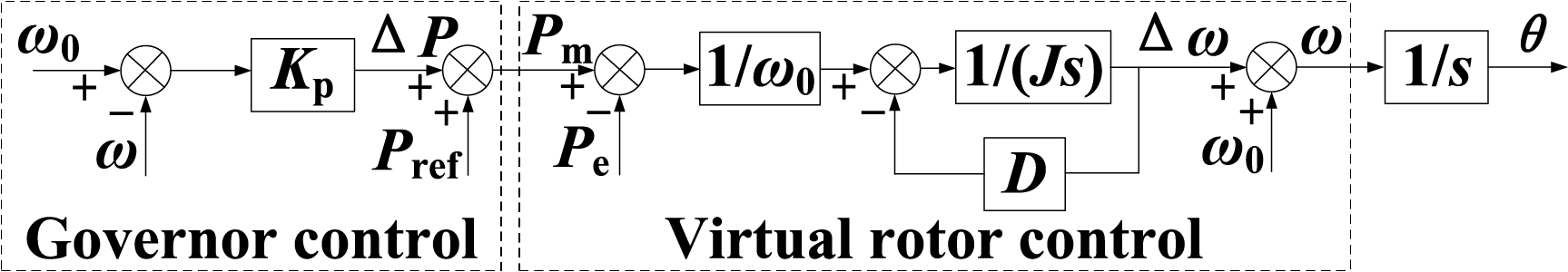
Figure 2: VSG active-frequency loop control block diagram
(2) Reactive power-voltage loop control
When the reactive power load increases in the system, synchronous generators increase their reactive power output to maintain system balance, resulting in a corresponding voltage drop. Conversely, when the reactive load decreases, the generator voltage rises.
The mathematical relationship between a synchronous generator’s reactive power output and its terminal voltage can be expressed by the following equation:
where:
U0 is the rated voltage amplitude, Q0 is the reactive power set value, and Kq is the synchronous generator reactive-voltage sag coefficient.
The reactive-voltage loop control of the VSG is formulated based on Eq. (3). To prevent voltage step changes during the regulation process, an inertial element 1/(kis) must be incorporated into the existing VSG excitation control system. This modification makes the dynamic response of the excitation regulation system more closely emulate the characteristics of a synchronous generator, ultimately generating the voltage reference signal Eref.
Fig. 3 illustrates the block diagram of the VSG reactive-voltage loop control.
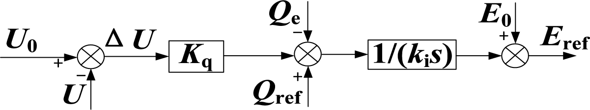
Figure 3: VSG reactive-voltage loop control block diagram
The expression for the voltage reference Eref can be derived from the above figure:
In the control architecture of the VSG, Eref represents the reference value of the virtual internal EMF, while ki denotes the integral gain within the reactive power control loop. Additionally, Kq is the reactive-voltage droop coefficient, U0 is the nominal voltage, and U represents the actual system output voltage. These control parameters collectively ensure that the voltage output accurately tracks the predefined reference value.
The active-frequency control loop generates a real-time phase angle signal, which is combined with the voltage reference signal from the reactive-voltage control loop to form the voltage command signal for the inner voltage-current double closed-loop control. The mathematical expression for the voltage command signal is provided below:
2.1.3 Inner Loop Double Closed Loop Vector Control
To enhance the system’s control performance, a voltage-current dual-loop control strategy is implemented. In the voltage outer loop, a quasi-proportional resonant control method is employed, enabling effective tracking of AC signals and achieving zero steady-state error control. For the current inner loop, proportional control is utilized to expedite the system’s dynamic response.
The voltage-current dual-loop control structure is illustrated in Fig. 4. In this configuration, the reference voltage uref from the outer loop is compared with the feedback voltage uc obtained from the filter capacitor. The resulting error signal is processed by the voltage controller Gu(s) to produce the reference current iref for the inner current loop. This reference current is then compared with the measured inductor current iL, and the error is fed into the proportional current controller Gi(s). The output of Gi(s) generates the necessary modulation signals to control the switching devices, ensuring accurate regulation of the switching process. The proportional controller Gi(s) plays a central role in enabling this precise and dynamic control mechanism.
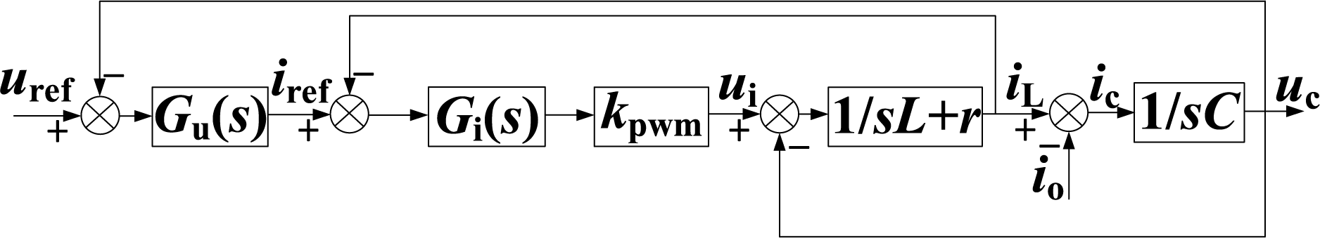
Figure 4: Block diagram of the voltage-current dual-loop control in the inner loop
2.2 VSG Control Parameter Analysis
2.2.1 VSG Power Ring Small Signal Modeling
The expressions for the active power (Pe) and reactive power (Qe) output by the VSG are presented as follows:
In Eq. (6), δ corresponds to the power angle of the VSG. Additionally, Zg and θg denote the equivalent impedance and its phase angle of the VSG filter circuit, respectively. These parameters are critical for characterizing the electrical behavior of the VSG, as they influence the power flow dynamics and stability of the system. The power angle δ plays a key role in determining the active power transfer, while the impedance Zg and its angle affect the voltage regulation and reactive power compensation capabilities of the VSG.
The expressions of Zg and θg are as follows:
where:
L1 denotes the inductance of the filter circuit, and R represents the output resistance of the VSG.
Adopting the analytical methodology used for small-signal modeling of synchronous generators [24], the output resistance of the VSG is assumed to be negligible. By combining the relationships described in Eqs. (1), (2) and (6), the small-signal model for the active power control loop of the VSG is developed. This model, which captures the dynamic behavior of the VSG under small disturbances, is graphically represented in Fig. 5.
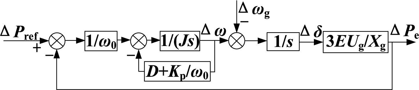
Figure 5: Small-signal control block diagram of the VSG closed-loop system
During the modeling process, the primary FM coefficient Kp shares a similar mathematical form with the damping coefficient D. To integrate these concepts, the notion of a damping droop coefficient D1 is introduced, defined as D1 = D + Kp/ω0. Based on Fig. 5, the closed-loop transfer function G(s) can be derived, which characterizes the response of the VSG to changes in the active power command value.
2.2.2 Impact of Virtual Inertia and Damping Coefficients on the Output Characteristics of Virtual Synchronous Generators
(1) Impact on Active Power Output Characteristics
The dynamic characteristics of the second-order system, including its natural oscillation frequency ωn and damping ratio ξ, are determined from the closed-loop transfer function G(s). This transfer function describes the system’s response to variations in the active power command of the VSG, as expressed in Eq. (8).
When the system exhibits underdamped behavior (0 < ξ < 1) and an error band of ±5% is specified, the system’s overshoot and settling time can be determined accordingly:
Eqs. (9) and (10) reveal that the dynamic response of the second-order system is primarily governed by two key parameters: the virtual inertia J and the effective damping coefficient D1. The latter, D1, is a composite parameter that combines the inherent damping coefficient D and the primary FM coefficient Kp. These parameters collectively define the system’s oscillatory behavior and its ability to attenuate disturbances. Specifically, the virtual inertia J influences the system’s natural frequency, while the effective damping coefficient D1 determines the rate of oscillation decay.
When the primary frequency modulation coefficient Kp and damping coefficient D are held constant, an increase in the virtual inertia parameter J leads to a higher overshoot (σ%) and an extended settling time (ts). On the other hand, if J remains unchanged, increasing both D and Kp reduces the overshoot (σ%) and decreases the settling time (ts). Fig. 6 demonstrates the active dynamic response curves of the system under different virtual regulation coefficients, where the arrows indicate the variation trend of active power as the parameters increase.
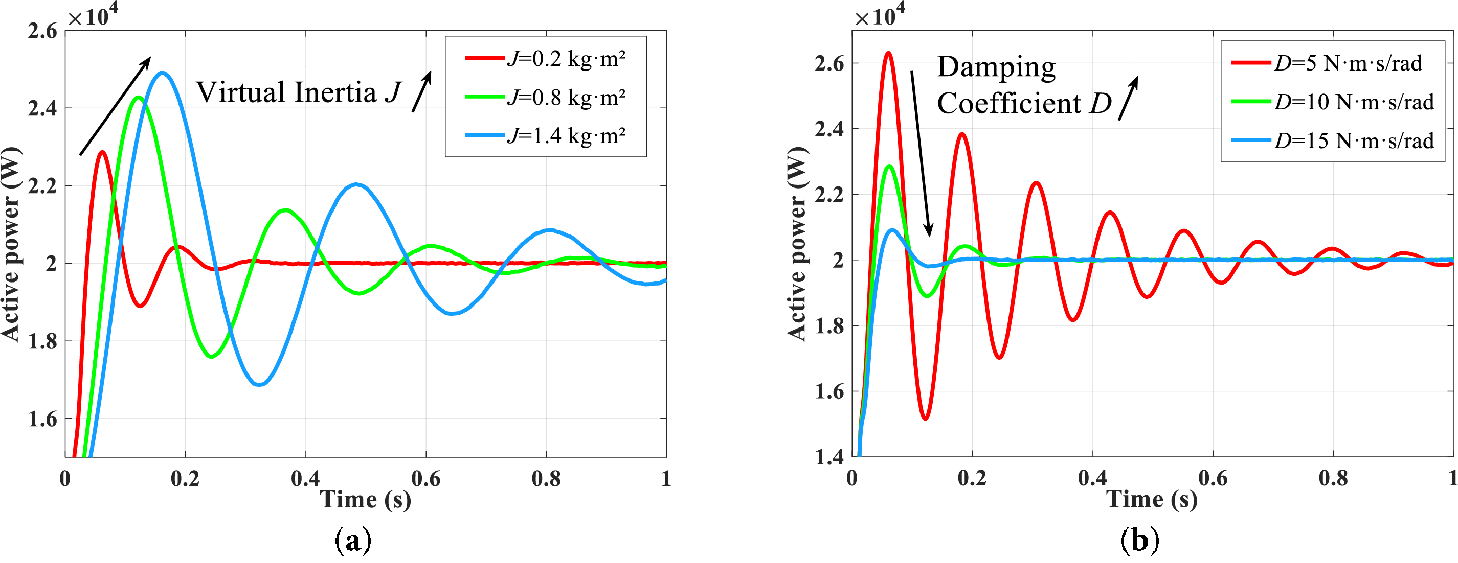
Figure 6: Dynamic response curves of active power output under different virtual adjustment coefficients. (a) Damping coefficient D = 10 N·m·s/rad. (b) Virtual inertia J = 0.2 kg·m2
According to the analysis above, the following conclusions can be drawn: The virtual inertia J primarily governs the oscillation frequency of the system, while the damping coefficient D determines the rate at which these oscillations diminish. Specifically, a larger J results in more frequent oscillations, whereas a higher D accelerates the decay of these oscillations. By carefully selecting appropriate values for J and D, the dynamic response performance of the active output can be significantly improved.
The following section further examines the influence of virtual inertia and damping coefficients on the dynamic response of the system’s active power output. Under a specified power command, the characteristic variation curve of the active power output dynamic response is illustrated in the accompanying figure. As depicted, an increase in J amplifies both the overshoot and settling time of the active power output. Additionally, under underdamped conditions, elevating D significantly reduces the overshoot and settling time of the power output, consistent with the simulation findings presented in Fig. 6. It is important to note that Fig. 7 demonstrates the ideal variation pattern of the active dynamic response influenced by virtual inertia and damping coefficients. Since virtual inertia and damping coefficients are affected by rotor angular frequency fluctuations and require continuous adjustment to suppress system frequency oscillations—necessitating consideration of their impact on system frequency—the overshoot and settling time cannot be reduced to zero.
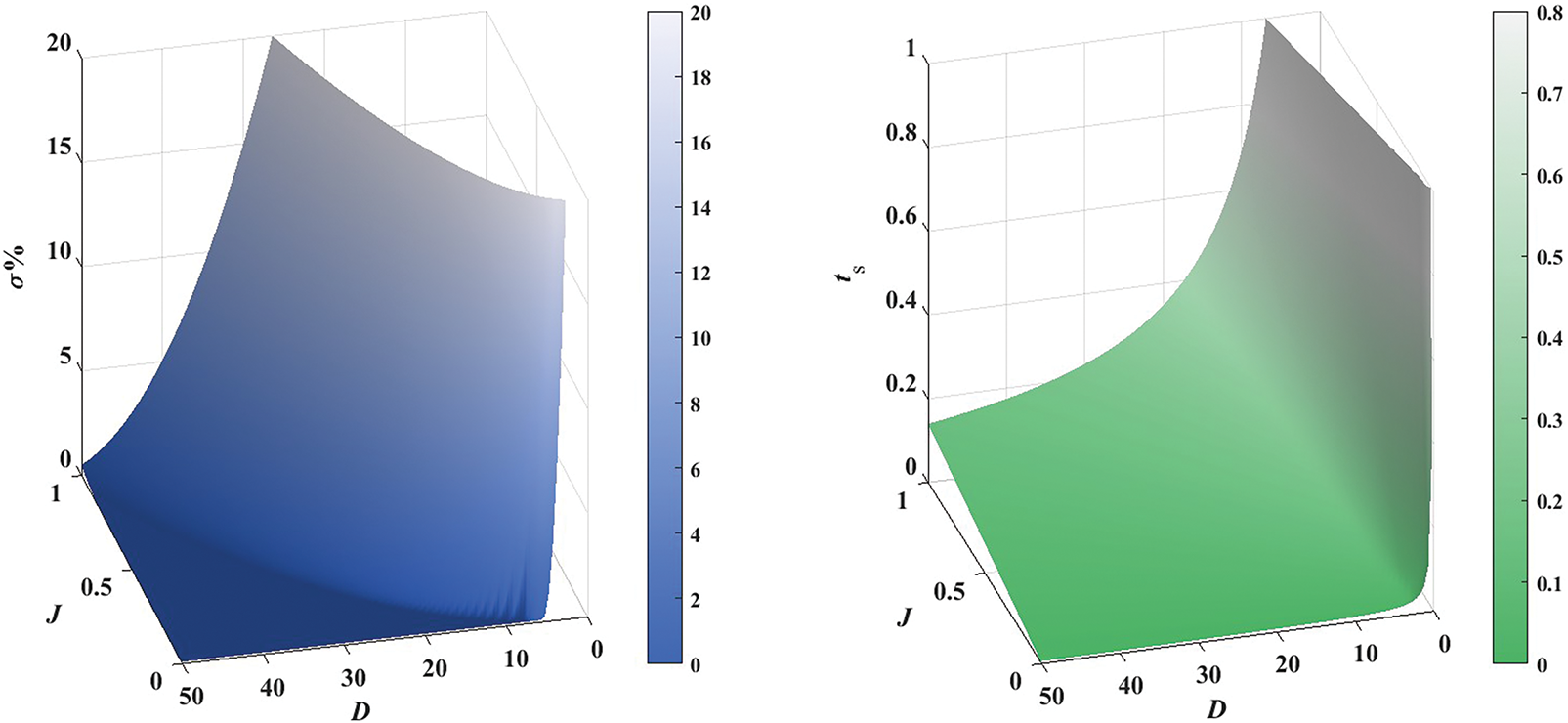
Figure 7: The influence of different J and D on the dynamic response characteristics of active power output
(2) The Effect on the Frequency Output Characteristics
According to Eq. (2) can be obtained:
Assuming the numerator on the right-hand side of Eqs. (11) and (12) remain constant, the damping coefficient D and the virtual inertia J exhibit inverse relationships with the angular velocity deviation Δω and the rate of change of angular velocity dω/dt, respectively. Specifically, a higher D results in a smaller Δω, while a larger J reduces dω/dt. By adjusting J and D, the system can effectively suppress angular frequency fluctuations, thereby improving its stability.
2.3.1 Characterization of Power and Angular Frequency under Small Perturbations
As demonstrated in the previous section, the inherent contradiction between transient and steady-state characteristics of a VSG cannot be resolved solely through parameter optimization. Specifically, while increasing the virtual inertia reduces angular frequency deviation, it simultaneously exacerbates power output overshoot and oscillations. Consequently, a mathematical framework must be developed to enable autonomous adjustment of key VSG parameters.
By emulating the electrical behavior of synchronous generators, VSGs exhibit power-angle curves and frequency oscillation curves analogous to their physical counterparts. When subjected to disturbances, the VSG control system determines its steady-state frequency according to the power-frequency droop curve. During transient regulation, two critical metrics govern system stability: transient settling time (ts) and overshoot magnitude (σ%) in the dynamic response. Fig. 8 illustrates the power angle characteristic curve and the angular frequency oscillation curve of the synchronous generator.
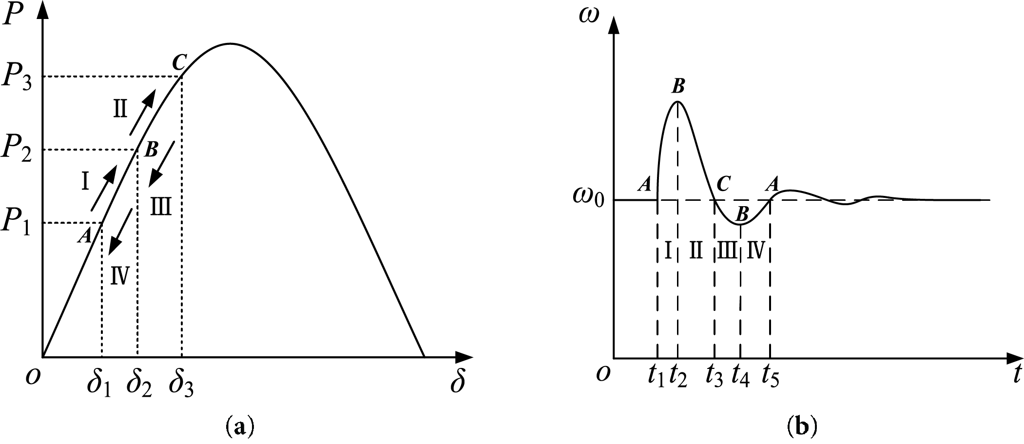
Figure 8: Synchronous generator power angle characteristic curve and angular frequency oscillation curve. (a) Power angle characteristic curve. (b) Angular frequency oscillation curve
In Fig. 8a, when the active input increases from P1 to P2, the system transitions from the initial steady-state point A to point B. This shift occurs through several decaying oscillation cycles. Driven by inertia, the system continues to evolve from point B to point C, eventually reaching a new steady state after additional decaying oscillations. According to the characteristics of the variation of the angular frequency in the figure, the first decay oscillation cycle is divided into four intervals: (I) t1–t2, (II) t2–t3, (III) t3–t4, and (IV) t4–t5.
During the first interval, the virtual rotor speed of the virtual synchronous generator is higher than the grid frequency and continues to increase. The rate of change of angular speed (dω/dt) initially experiences a sudden rise before gradually decreasing. To prevent excessive dω/dt and speed deviation (Δω) during this interval, it is necessary to increase both the virtual inertia (J) and the damping coefficient (D).
In the second interval, the virtual rotor speed enters a deceleration phase (dω/dt < 0), where the speed gradually decreases from its peak value while remaining above the grid reference frequency (ω > ω0). During this stage, it is advisable to reduce the virtual inertia to accelerate the restoration of angular velocity to its rated value, while simultaneously increasing the damping coefficient when Δω remains large to suppress angular velocity deviation further.
The selection criteria for the virtual inertia and damping coefficient parameters in Intervals III and IV follow the same principles as those for Intervals I and II, and thus will not be reiterated here.
2.3.2 Parameter Adaptive Control Regulation Principle
As illustrated in Section 2.3.1, the virtual inertia value is determined by both the rate of change of angular frequency and its deviation, while the damping coefficient is solely dependent on the angular frequency deviation. Table 2 summarizes the adjustment principles for the virtual inertia and damping coefficient across different operational stages.
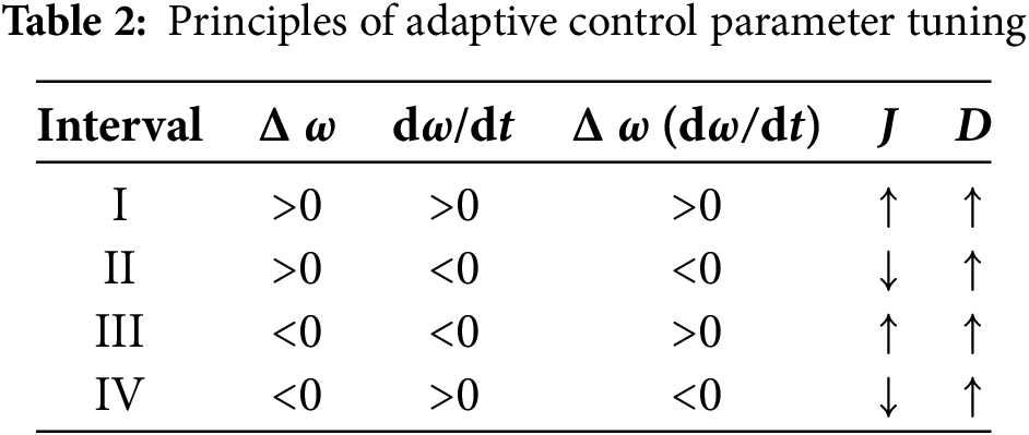
According to the principles of adaptive control parameter adjustment in Table 2, the computational expressions for determining the magnitude of the values of the virtual inertia and damping coefficient are given:
where:
J0 and D0 represent the virtual inertia and damping coefficients of the VSG under stable operating conditions, respectively. Kj and Kd are the adjustment coefficients for virtual inertia and damping, while Tj and Td denote the threshold limits for the rate of change of angular frequency and angular frequency deviation, respectively. The flowchart of the control strategy is shown in Fig. 9.
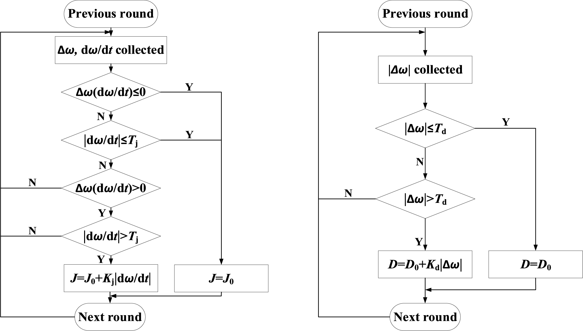
Figure 9: Adaptive control flowchart
The selection of these thresholds is crucial for the system’s steady-state performance. Appropriately chosen thresholds ensure that the system remains robust against frequent variations in control parameters. Through adaptive tuning of these key parameters, the dynamic performance of the system can be significantly improved. The principle of inertia damping adaptive control is shown in Fig. 10.
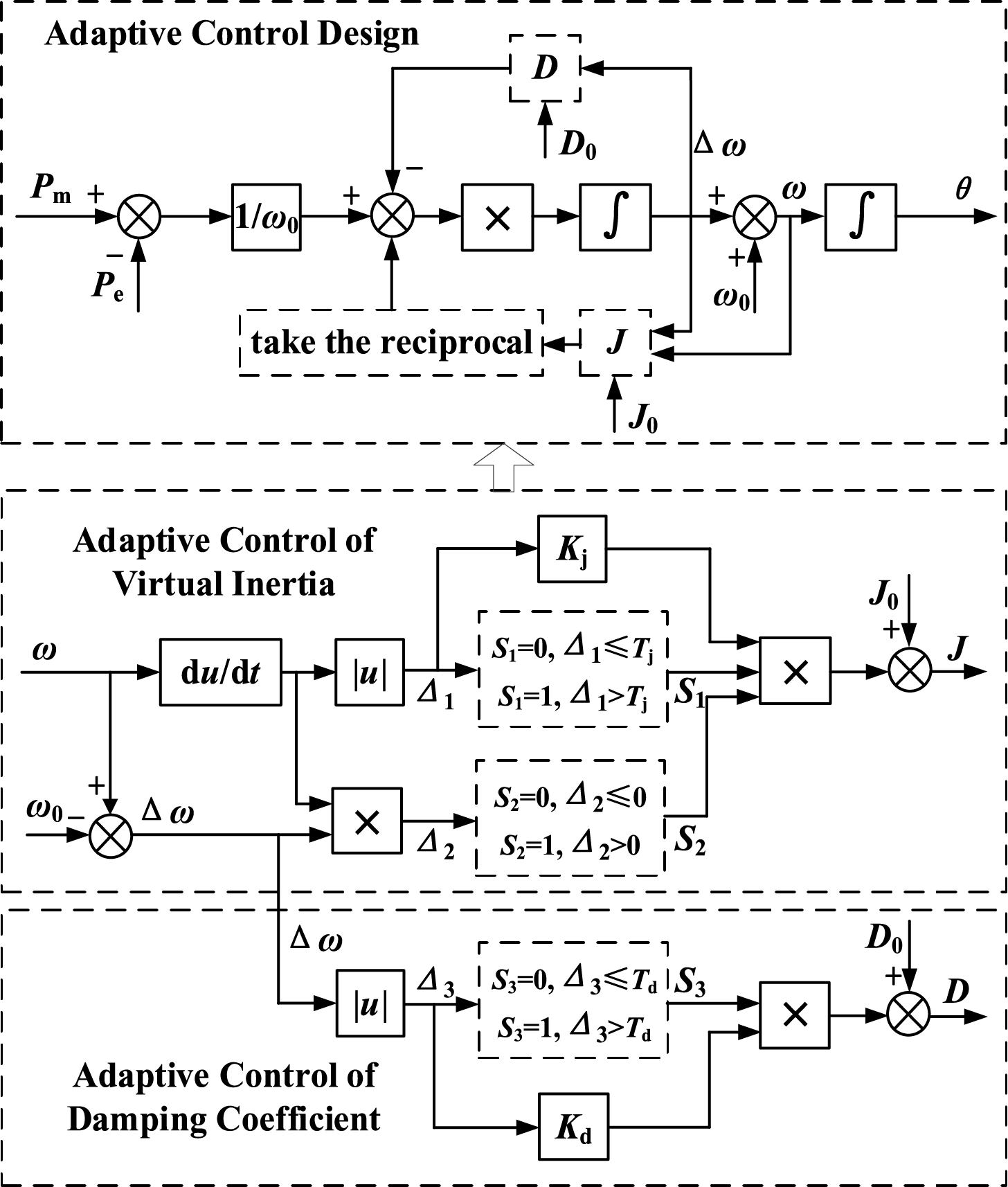
Figure 10: Schematic diagram of adaptive control for virtual parameters
2.3.3 Controller Parameterization
The characteristic root of the transfer function of the equivalent second-order system is obtained from Eq. (8) as:
The open-loop transfer function of the system can be obtained from Fig. 5:
According to Eqs. (15) and (16), the distribution of system poles under parameter variation is derived, and the pole distribution is shown in Fig. 11, where the arrows indicate the movement trajectories of the conjugate poles s1 and s2.
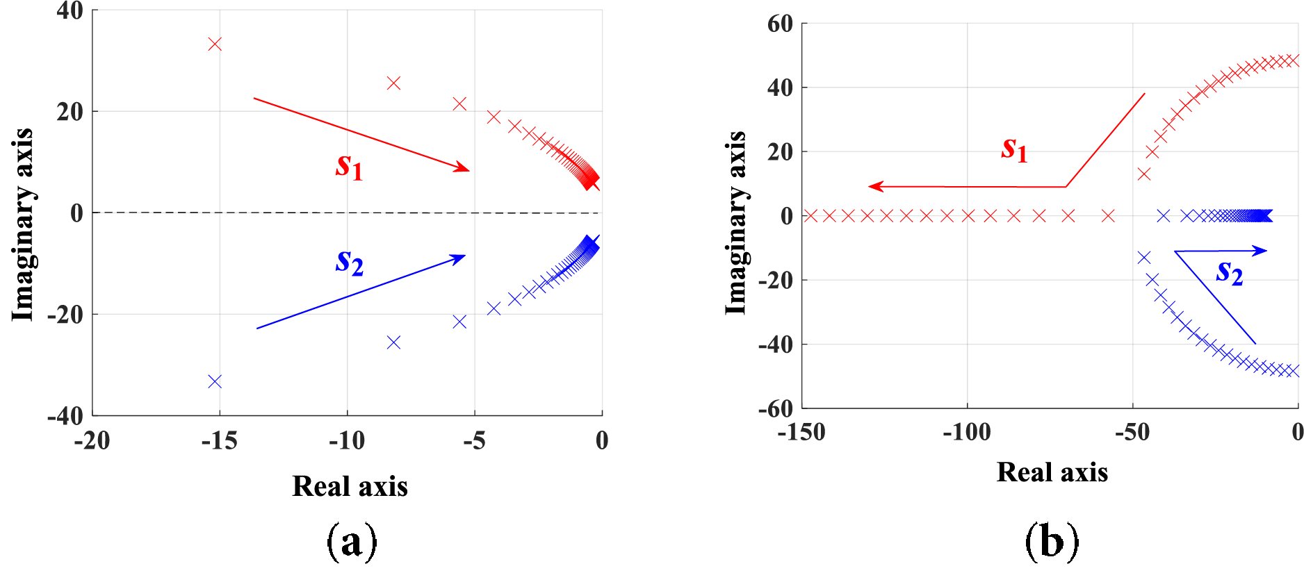
Figure 11: Pole distribution of the system with parameter variation. (a) Change in virtual inertia. (b) Change in damping coefficient
When D is held constant and J is increased from 0.05 to 15, the distribution of the system’s poles is depicted in Fig. 11a. According to Liapunov stability theory, system stability is ensured when the poles are located in the left half-plane. As observed from the figure, the conjugate poles gradually approach the imaginary axis, with a faster movement near the imaginary axis compared to the real axis. This trend indicates a degradation in system stability. When the virtual inertia exceeds a certain threshold, the pole distribution becomes more concentrated. At this stage, further adjustments to the virtual inertia have minimal impact on system stability.
When J is held constant and D is increased from 0 to 50, the pole distribution of the system is shown in Fig. 11b. As the damping coefficient increases, the conjugate poles shift towards the negative real axis in the left half-plane. During this phase, the damping ratio increases, leading to a reduction in overshoot and an improvement in the system’s dynamic response performance. However, when the damping coefficient D exceeds a certain threshold, the system transitions from underdamped to overdamped. The response time increases, and the original conjugate poles separate along the negative real axis. The dominant pole moves closer to the imaginary axis, resulting in deteriorated system stability.
Building on KU Leuven’s virtual synchronous generator architecture, during the initial grid frequency deviation, virtual inertial power becomes the dominant part, during which the inverter primarily supplies inertial power. Compliance with the following formulation enables full utilization of the inverter’s capacity:
The stability margin of the system can be evaluated by analyzing the location of its poles. Specifically, the greater the distance of the poles from the imaginary axis, the higher the system’s stability margin. To guarantee system stability, the pole locations must adhere to the following equation:
In this study, the virtual inertia J0 is configured as 0.2 kg·m2, and the damping coefficient D0 is set to 10 N·m·s/rad. The adjustment coefficients Kj and Kd, along with the threshold values Tj for the rate of change of angular velocity and Td for angular velocity deviation, are determined according to specific application needs.
3.1 Parameter Sensitivity Study on Frequency Fluctuation Characteristics
Eqs. (13) and (14) reveal that the magnitudes of the regulation coefficients Kj and Kd directly affect the system’s capability to suppress frequency fluctuations, and the upper limits for the values of Kj and Kd can be preliminarily derived by modifying Eqs. (13) and (14):
Regarding the adaptive control strategy studied in this paper, the derivation process for the design principles of parameters Kj and Kd is as follows.
Based on Eq. (13), Kj can be expressed through Eq. (20):
Therefore:
Neglecting the damping term in Eq. (2) yields:
The above equation indicates that:
Combining Eqs. (21) and (23) gives:
It can be concluded that when implementing the inertia-damping adaptive control strategy, after determining J0 during steady-state operation, the inertia adaptation parameters are primarily determined by the maximum capacity constraints and the allowable maximum frequency deviation. In practical engineering applications, both the VSG dynamic response characteristics and the permissible external disturbance range must be simultaneously considered; therefore, it is recommended that Kj be selected within the range (0, 0.8Kjmax].
As introduced previously regarding the concept of damping droop coefficients, and combined with the Kj parameter design principles:
The expression for angular frequency deviation during stable operation is:
Combining Eqs. (25) and (26) yields:
Similarly, Kd selection follows analogous design principles to Kj. It is generally recommended that Kd be chosen within the range (0, 0.8Kdmax].
The specific parameter values will be further determined based on simulation results. During testing, the active power output of the VSG is maintained at 20 kW. When Kj is varied, Kd is fixed at 10; conversely, when Kd is adjusted, Kj remains constant at 0.2.
The influence of these parameter variations on system frequency is depicted in Fig. 12, where the arrows indicate the trend of system frequency variation as the control parameter increases.
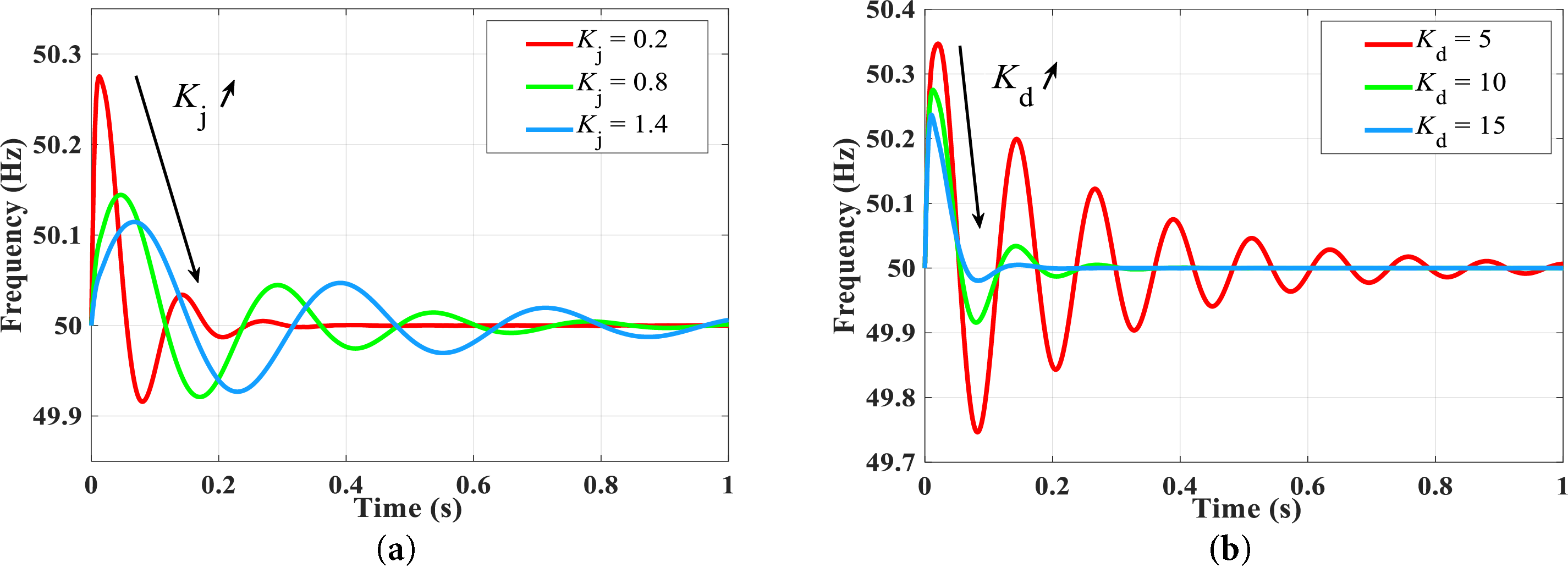
Figure 12: Frequency fluctuation of the system with different virtual inertia and damping adjustment coefficients. (a) Kd = 10 with varying Kj. (b) Kj = 0.2 with varying Kd
As shown in Fig. 12, when Kd = 10 and Kj takes the values of 0.2, 0.8, and 1.4, the time for the system to reach the first oscillation peak is 0.0125, 0.0464 and 0.0673 s, respectively. The maximum oscillation amplitude of the frequency when Kj = 0.2 and Kd takes the values of 5, 10, and 15 is about 50.347, 50.275 and 50.237 Hz, respectively. This indicates that with the increase of the adjustment coefficients Kj and Kd, the rate of change of the VSG rotor frequency gradually slows down, and the overshoot amplitude decreases. Kj characterizes the frequency response capability of the inertia constant J. An excessively large Kj value may lead to overshoot in J during transient states, potentially compromising the system’s dynamic response. Thus, a conservative Kj value is selected here. The damping coefficient Kd controls the effectiveness of D in tracking frequency deviations. An excessively high Kd may lead to VSG over-damping, increasing the damping ratio and prolonging the settling time while degrading transient performance. Based on comprehensive frequency response analysis, the optimal Kd value is determined as 10 for this study.
For the selection of Tj and Td values, specifically during normal VSG operation, the system’s angular frequency exhibits minor fluctuations where the rate of angular frequency change cannot be neglected. As the threshold for angular frequency rate of change, Tj determines whether to trigger the adaptive inertia switching. To prevent false operations during normal operation, Tj must exceed the maximum angular frequency rate of change during stable VSG operation. Meanwhile, to maintain the adaptive system’s precision, Tj should not be excessively large, it only needs to satisfy the requirement of avoiding false triggering. Similar principles apply for determining Td, the threshold for angular frequency deviation. In this study, the values of Tj and Td are selected as 2 and 0.1, respectively.
3.2 Inertia-Damping Adaptive Control Strategy
3.2.1 Active Power Command Variation Condition
This study conducts a comparative analysis of the power and frequency responses of the VSG system under four distinct control strategies: fixed-parameter control, adaptive virtual inertia control, adaptive damping coefficient control, and coordinated adaptive control of both inertia and damping.
The VSG grid-connected model is developed in the MATLAB/Simulink environment, and relevant simulation experiments are carried out. The simulation parameters are provided in detail in Table 3.
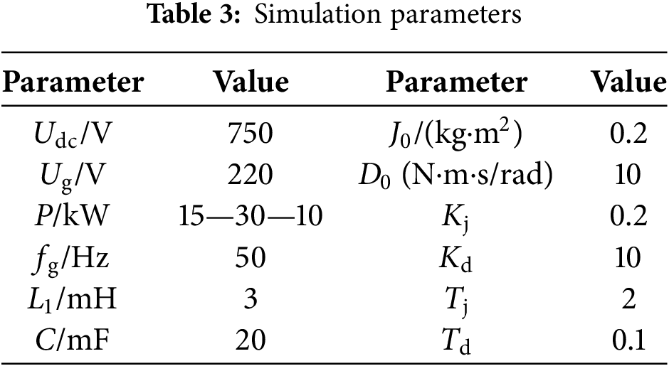
The simulation experiment is conducted over 1 s. Initially, the active power output of the VSG is set at 15 kW. At 0.2 s, the active power abruptly increases to 30 kW, and then sharply drops to 10 kW at 0.6 s.
Fig. 13 displays the current output waveforms for the four control methods under study. The traditional control method, which emulates the inertia and damping characteristics of synchronous generators, exhibits current overshoot and oscillations during power command transitions. The adaptive inertia control method effectively suppresses these overshoots and oscillations. While the adaptive damping control eliminates overshoot and oscillation completely, it results in less smooth current transitions. The inertia-damping adaptive control combines the benefits of both approaches, delivering smooth current variations during power command changes without noticeable overshoot or oscillation, demonstrating superior dynamic response performance.
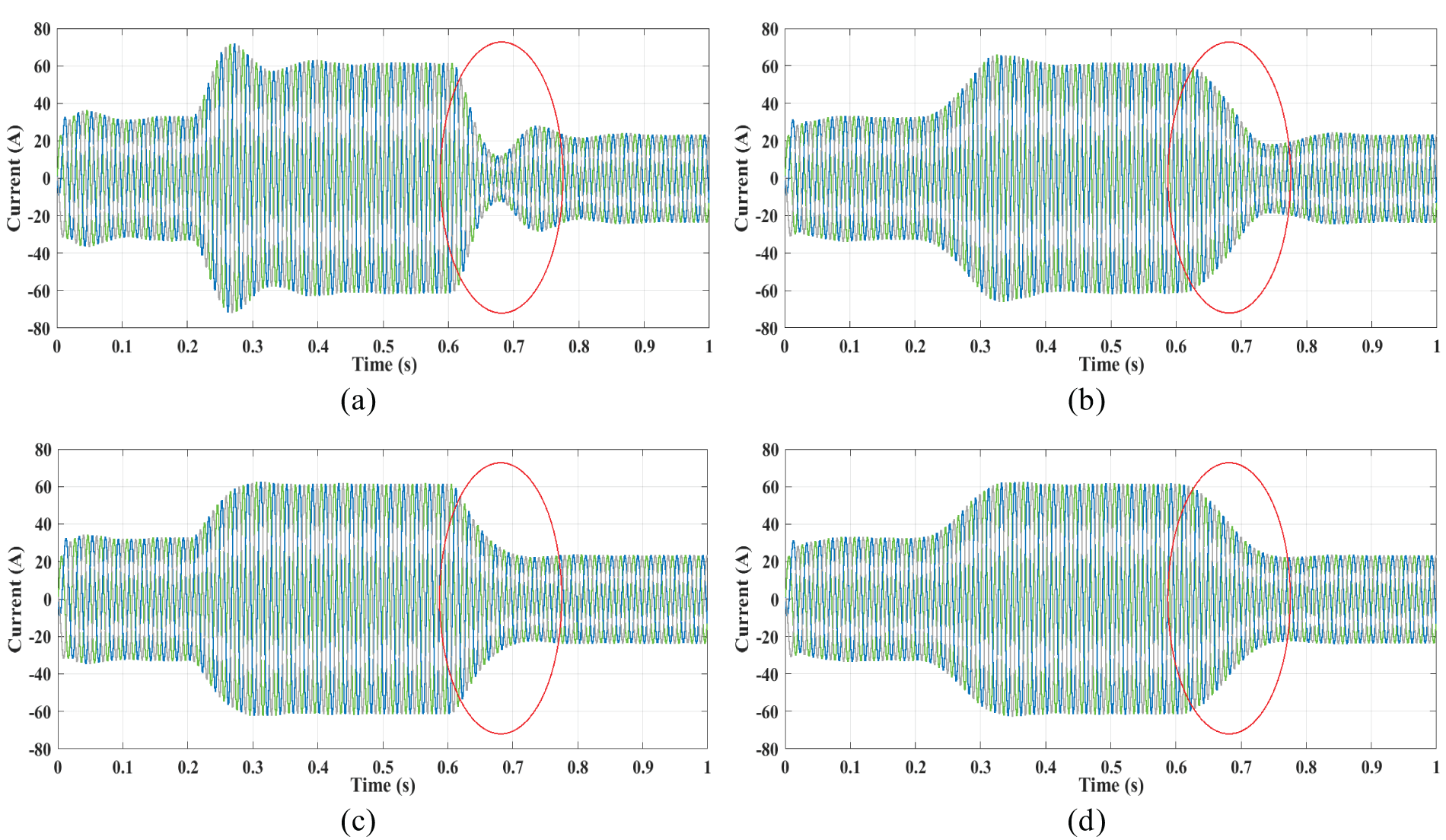
Figure 13: Simulation current waveform. (a) Traditional VSG control. (b) Inertia adaptive VSG control. (c) Damping adaptive VSG control. (d) Inertia-damping adaptive VSG control
Fig. 14 presents the dynamic response curves of the active output of the VSG under different control strategies. Facing the sudden increase of the input power, the overshoot of the output active power of the three control strategies, fixed parameter control, adaptive rotational inertia control, and coordinated adaptive control, decreases in order, which are 36%, 15.6%, and 3.4%, respectively. Accordingly, the time required for these control strategies to reach the steady state is also different, about 0.21, 0.19 and 0.12 s. The overshooting amount of the adaptive damping coefficient control is 3.5%, and the settling time is about 0.08 s. Compared with the inertia-damping coordinated adaptive control, the response is faster, which is the optimal performance among the four control strategies, and is analyzed in conjunction with the effect on the frequency of the system.
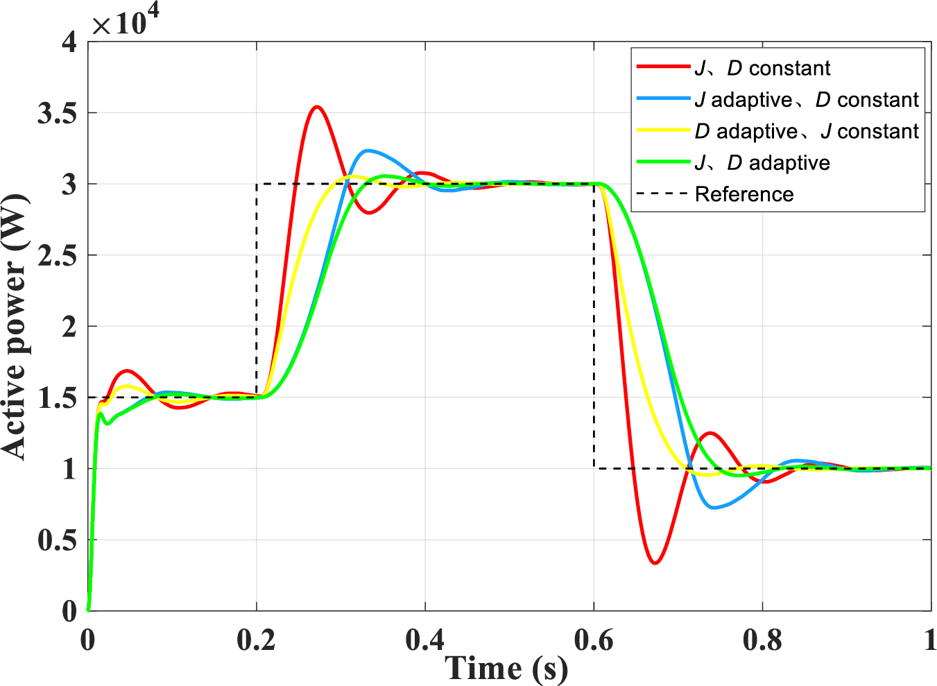
Figure 14: Dynamic response curve of active output under different control strategies
Fig. 15 shows the comparative analysis of the output frequency of the VSG with different control strategies. The maximum frequency amplitudes of the four control strategies are 50.46, 50.21, 50.25, and 50.17 Hz, respectively. As shown in the figure, the adaptive virtual inertia control and adaptive damping coefficient control are better than the traditional fixed parameter control. Further comparison reveals that the synergistic combined control strategy of virtual inertia and damping coefficient can significantly improve the system performance. Specifically, this combined control approach not only shortens the time required for the system to reach the steady state condition but also minimizes the frequency deviation.
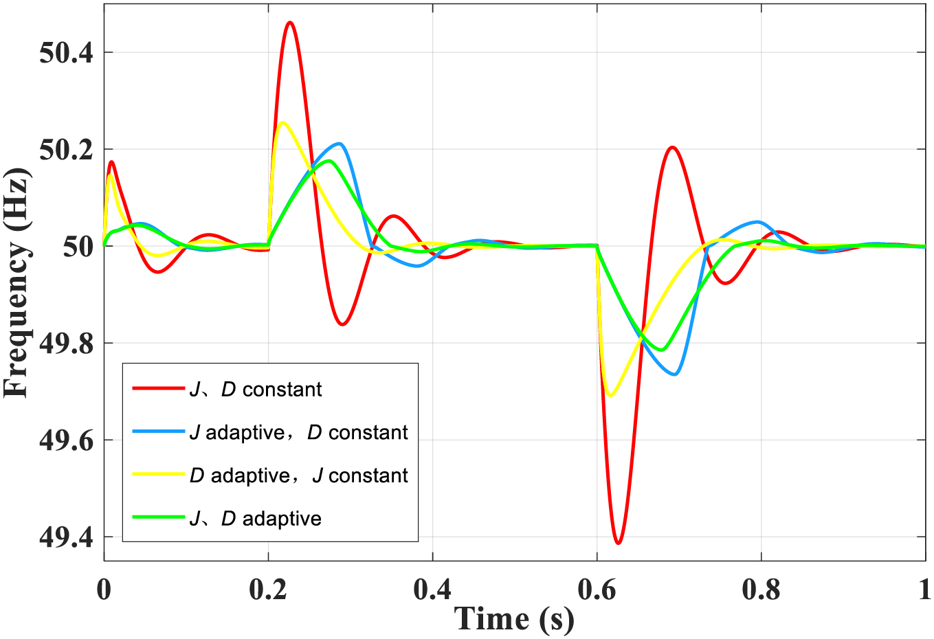
Figure 15: Frequency comparison under different control strategies
Based on the simulation results of Figs. 14 and 15, the quantitative metrics of different control strategies can be concluded in Table 4.
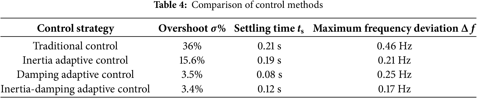
Fig. 16 illustrates the dynamic changes in virtual inertia and damping coefficient during the adaptive control process. Once the system achieves stability, the adjusted parameters revert to their initial values. The proper selection of control parameters effectively mitigates excessive virtual inertia regulation to some extent.
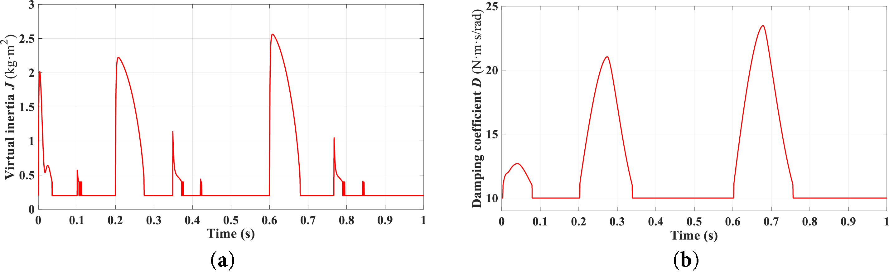
Figure 16: Adaptive curve of virtual inertia and damping coefficient. (a) Virtual inertia J. (b) Coefficient of damping D
In summary, while adaptive damping coefficient control excels in enhancing the dynamic response performance of the system’s active output, the adaptive control strategy that integrates both virtual inertia and damping coefficient offers a more comprehensive improvement. This integrated approach not only mitigates system overshoot and enhances dynamic performance but also reduces the amplitude of frequency fluctuations and frequency deviations.
3.2.2 Load Step Change Conditions
Fig. 17 demonstrates the frequency regulation performance under load step changes. With the active power command maintained at 20 kW, the system experiences a load step increase from 5 to 10 kW at 0.3 s, followed by a step decrease back to 5 kW at 0.7 s, while keeping all other parameters consistent with Table 3. Under these load disturbances, the conventional VSG control exhibits significant power oscillations, resulting in grid frequency fluctuations of approximately 0.2 Hz. In contrast, the proposed adaptive control strategy substantially improves system stability. The adaptive parameters dynamically adjust to suppress power overshoot and mitigate frequency oscillations. When a load step change occurs, the adaptive controller rapidly compensates for the active power imbalance, ensuring smooth frequency regulation without oscillatory behavior. Consequently, the grid frequency fluctuation amplitude is effectively reduced to less than 0.1 Hz, demonstrating superior dynamic performance compared to conventional control methods.
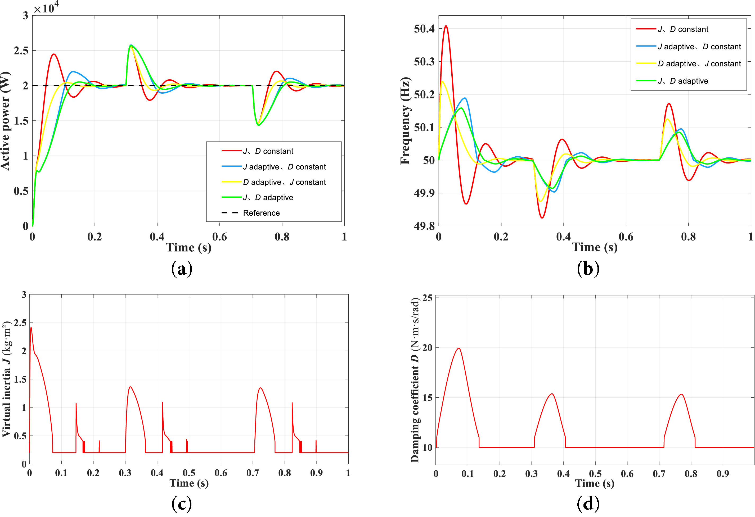
Figure 17: Characteristic curves of VSG dynamic parameters under load step change conditions. (a) Active power. (b) Frequency. (c) Virtual inertia J. (d) Coefficient of damping D
3.2.3 Large-Grid Voltage Sag Condition
Fig. 18 shows the dynamic response curve of the VSG under a large grid voltage sag condition. Initially, the inverter operates normally in grid-connected mode. At 0.5 s, a grid fault causes a symmetrical voltage drop to 0.5 p.u. As can be seen from the figure, the voltage sag has a significant impact on the power output of the VSG, resulting in a severe transient power overshoot within a short period. The adaptive control strategy smooths the power output of the VSG to some extent, but its response speed is slower compared to the other three control methods. In terms of system stability, the adaptive control strategy is more effective in suppressing frequency fluctuations than the other three control strategies, significantly improving grid stability.
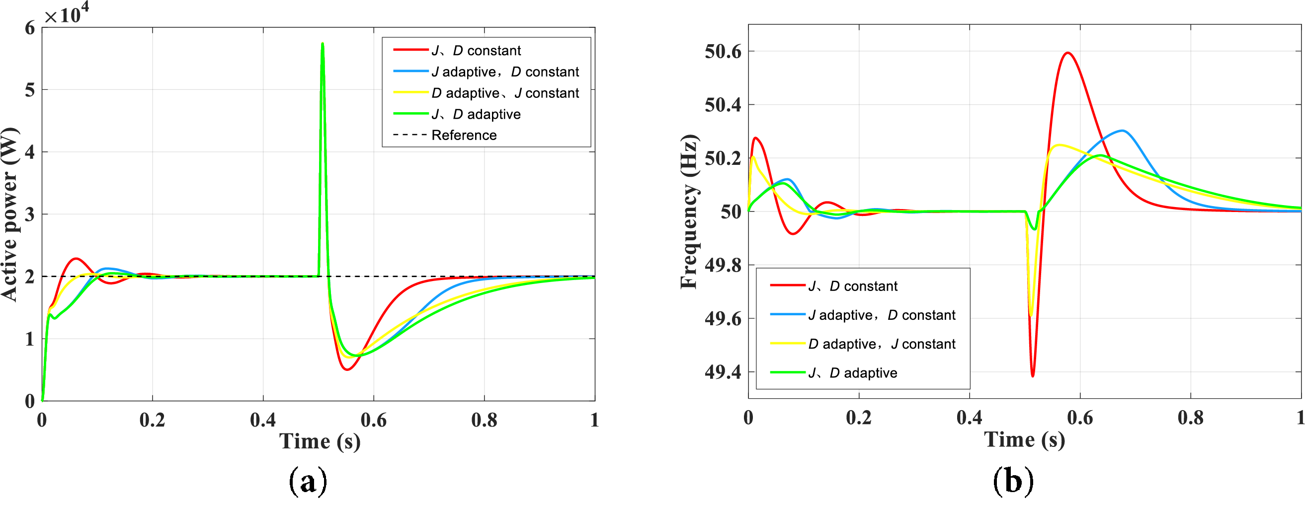
Figure 18: Dynamic response curves of VSG under large-grid voltage sag conditions. (a) Active power. (b) Frequency
Fig. 19 shows the voltage and current waveforms output by the inverter. Under large grid voltage sags, maintaining constant active power output from the inverter can lead to output currents far exceeding the rated value. In practical applications, this may trigger protective devices to disconnect the inverter from the grid, thereby losing its grid support capability—and in severe cases, potentially damaging the inverter. While enhancing the low-voltage ride-through (LVRT) capability of virtual synchronous generators represents a separate research direction beyond the scope of this study, the simulation results demonstrate that the proposed adaptive control strategy effectively improves grid frequency stability during severe voltage sags.
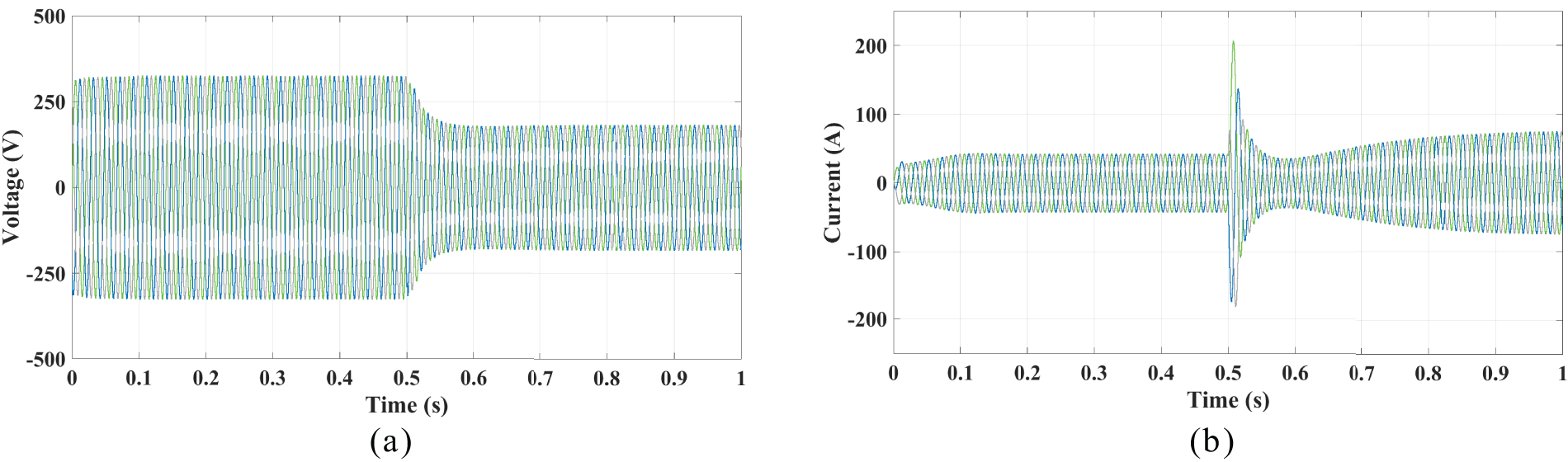
Figure 19: Voltage and current output curves of VSG under large-grid voltage sag conditions. (a) Voltage output. (b) Current output
This study proposes a multi-stage adaptive control strategy for virtual inertia (J) and damping coefficients (D) based on the power characteristics of VSG. The core innovation lies in dynamically adjusting both J and D through explicit control expressions, effectively suppressing both the rate of change of angular frequency (dω/dt) and steady-state deviation (Δω). Root locus analysis reveals that increasing virtual inertia degrades system stability and slows convergence, while higher damping enhances stability but prolongs settling time. MATLAB/Simulink simulations further confirm that J governs transient oscillation frequency, whereas D determines the attenuation rate. Compared to fixed-parameter and single-parameter adaptive methods, the proposed strategy reduces the frequency deviation from 0.46 to 0.17 Hz and shortens the active power response settling time from 0.21 to 0.12 s. Additional tests verify the control strategy’s effectiveness under both load variation and grid voltage sag conditions.
However, the adaptive control strategy proposed in this paper, while capable of improving system stability under large grid voltage sag conditions, has minimal impact on power output regulation under such conditions. To fundamentally address this issue, a LVRT control strategy needs to be introduced. Furthermore, the current adaptive control strategy has only been implemented in a single VSG inverter unit. For multi-VSG parallel systems, the required damping coefficients and virtual inertia may vary under different operating conditions. Subsequent research should focus on optimizing the adaptive control strategy to effectively suppress power circulation and oscillation phenomena in multi-parallel VSG systems and improve power distribution among units.
Additionally, it is worth noting that advances in intelligent control, machine learning, and deep learning offer new approaches for the adaptive parameter optimization discussed in this study. These techniques show potential for further optimizing power output performance and enhancing frequency stabilization capabilities, but their implementation significantly increases control model complexity: multi-output configurations escalate rule dimensionality, computational load, and model training time. Besides, depending on the specific rules and algorithms developed, they may not simultaneously optimize both power output and frequency fluctuation suppression, and their applicability is limited to certain operating conditions. Consequently, these approaches remain some distance from practical engineering implementation, combining these novel control approaches with the method proposed in this paper to address the challenge of multi-parameter coordination control could also be one of the future research directions.
Acknowledgement: We would like to thank all the authors for their guidance and help on this article.
Funding Statement: This work is financially supported by the Talent Initiation Fund of Wuxi University (550220008).
Author Contributions: Study conception and design: Jin Lin, Bin Yu; data collection: Jin Lin, Chao Chen, Yifan Wu; analysis and interpretation of results: Jin Lin, Bin Yu, Jiezhen Cai; draft manuscript: Jin Lin, Jiezhen Cai; manuscript revision: Jin Lin; academic supervision: Cunping Wang. All authors reviewed the results and approved the final version of the manuscript.
Availability of Data and Materials: The data and supportive information are available within the article.
Ethics Approval: Not applicable.
Conflicts of Interest: The authors declare no conflicts of interest to report regarding the present study.
References
1. Mahmoud MS. Microgrid: advanced control methods and renewable energy system integration. Amsterdam, The Netherlands: Elsevier; 2016. [Google Scholar]
2. Zhang Y, Ma T, Yang H. Grid-connected photovoltaic battery systems: a comprehensive review and perspectives. Appl Energy. 2022;328(8):120182. doi:10.1016/j.apenergy.2022.120182. [Google Scholar] [CrossRef]
3. Tahir W, Farhan M, Bhatti AR, Butt AD, Farid G. A modified control strategy for seamless switching of virtual synchronous generator-based inverter using frequency, phase, and voltage regulation. Int J Electr Power Energy Syst. 2024;157(17):109805. doi:10.1016/j.ijepes.2024.109805. [Google Scholar] [CrossRef]
4. Tamrakar U, Shrestha D, Maharjan M, Bhattarai B, Hansen T, Tonkoski R. Virtual inertia: current trends and future directions. Appl Sci. 2017;7(7):654. doi:10.3390/app7070654. [Google Scholar] [CrossRef]
5. Fernández-Guillamón A, Gómez-Lázaro E, Muljadi E, Molina-García Á. Power systems with high renewable energy sources: a review of inertia and frequency control strategies over time. Renew Sustain Energy Rev. 2019;115(6–7):109369. doi:10.1016/j.rser.2019.109369. [Google Scholar] [CrossRef]
6. Cheema KM. A comprehensive review of virtual synchronous generator. Int J Electr Power Energy Syst. 2020;120:106006. doi:10.1016/j.ijepes.2020.106006. [Google Scholar] [CrossRef]
7. Chen M, Zhou D, Wu C, Blaabjerg F. Characteristics of parallel inverters applying virtual synchronous generator control. IEEE Trans Smart Grid. 2021;12(6):4690–701. doi:10.1109/TSG.2021.3102994. [Google Scholar] [CrossRef]
8. Wang F, Zhang L, Feng X, Guo H. An adaptive control strategy for virtual synchronous generator. IEEE Trans Ind Appl. 2018;54(5):5124–33. doi:10.1109/TIA.2018.2859384. [Google Scholar] [CrossRef]
9. Li M, Huang W, Tai N, Yang L, Duan D, Ma Z. A dual-adaptivity inertia control strategy for virtual synchronous generator. IEEE Trans Power Syst. 2020;35(1):594–604. doi:10.1109/TPWRS.2019.2935325. [Google Scholar] [CrossRef]
10. Wu H, Wang X. A mode-adaptive power-angle control method for transient stability enhancement of virtual synchronous generators. IEEE J Emerg Sel Top Power Electron. 2020;8(2):1034–49. doi:10.1109/JESTPE.2020.2976791. [Google Scholar] [CrossRef]
11. Liang X, Andalib-Bin-Karim C, Li W, Mitolo M, Shabbir MNSK. Adaptive virtual impedance-based reactive power sharing in virtual synchronous generator controlled microgrids. IEEE Trans Ind Appl. 2021;57(1):46–60. doi:10.1109/TIA.2020.3039223. [Google Scholar] [CrossRef]
12. Yin G, Dong H, Dai Y, Wang H, Wang S. Parameter adaptive control strategy of virtual synchronous generator in photovoltaic microgrid. Power Syst Technol. 2019;44(1):192–9. (In Chinese). doi:10.13335/j.1000-3673.pst.2018.3031. [Google Scholar] [CrossRef]
13. He X, Zuo Y, Yang Y, Liu C, Zhou X, Wang D. Research on grid-connected inverter control strategy based on adaptive parameter adjustment of virtual synchronous generator. Acta Energiae Solaris Sin. 2024;45(7):259–66. (In Chinese). doi:10.19912/j.0254-0096.tynxb.2023-0496. [Google Scholar] [CrossRef]
14. Li J, Wen B, Wang H. Adaptive virtual inertia control strategy of VSG for micro-grid based on improved Bang-Bang control strategy. IEEE Access. 2019;7:39509–14. doi:10.1109/access.2019.2904943. [Google Scholar] [CrossRef]
15. Shuai Z, Shen C, Liu X, Li Z, Shen ZJ. Transient angle stability of virtual synchronous generators using Lyapunov’s direct method. IEEE Trans Smart Grid. 2019;10(4):4648–61. doi:10.1109/TSG.2018.2866122. [Google Scholar] [CrossRef]
16. Karimi A, Khayat Y, Naderi M, Dragičević T, Mirzaei R, Blaabjerg F, et al. Inertia response improvement in AC microgrids: a fuzzy-based virtual synchronous generator control. IEEE Trans Power Electron. 2020;35(4):4321–31. doi:10.1109/TPEL.2019.2937397. [Google Scholar] [CrossRef]
17. Shang L, Hu J, Yuan X, Chi Y, Tang H. Modeling and improved control of virtual synchronous generator under symmetrical grid fault. Proc CSEE. 2017;37(2):403–12. (In Chinese). doi:10.13334/j.0258-8013.pcsee.162201. [Google Scholar] [CrossRef]
18. Ren B, Li Q, Fan Z, Sun Y. Adaptive control of a virtual synchronous generator with multiparameter coordination. Energies. 2023;16(12):4789. doi:10.3390/en16124789. [Google Scholar] [CrossRef]
19. Grover H, Sharma S, Verma A, Hossain MJ, Kamwa I. Adaptive parameter tuning strategy of VSG-based islanded microgrid under uncertainties. Electr Power Syst Res. 2024;235(4):110854. doi:10.1016/j.epsr.2024.110854. [Google Scholar] [CrossRef]
20. Long B, Liao Y, Chong KT, Rodríguez J, Guerrero JM. Enhancement of frequency regulation in AC microgrid: a fuzzy-MPC controlled virtual synchronous generator. IEEE Trans Smart Grid. 2021;12(4):3138–49. doi:10.1109/TSG.2021.3060780. [Google Scholar] [CrossRef]
21. Yao F, Zhao J, Li X, Mao L, Qu K. RBF neural network based virtual synchronous generator control with improved frequency stability. IEEE Trans Ind Inform. 2021;17(6):4014–24. doi:10.1109/TII.2020.3011810. [Google Scholar] [CrossRef]
22. Wang Y, Song F, Ma Y, Zhang Y, Yang J, Liu Y, et al. Research on capacity planning and optimization of regional integrated energy system based on hybrid energy storage system. Appl Therm Eng. 2020;180(6390):115834. doi:10.1016/j.applthermaleng.2020.115834. [Google Scholar] [CrossRef]
23. Yang H, Shao T, Yin Z. Hybrid energy storage for mitigating photovoltaic output voltage fluctuations based on EEMD. Electr Eng. 2022;8:50–2+131. (In Chinese) doi:10.19768/j.cnki.dgjs.2022.08.018. [Google Scholar] [CrossRef]
24. Wu H, Ruan X, Yang D, Chen X, Zhao W, Lv Z, et al. Small-signal modeling and parameters design for virtual synchronous generators. IEEE Trans Ind Electron. 2016;63(7):4292–303. doi:10.1109/TIE.2016.2543181. [Google Scholar] [CrossRef]
Cite This Article
 Copyright © 2026 The Author(s). Published by Tech Science Press.
This work is licensed under a Creative Commons Attribution 4.0 International License , which permits unrestricted use, distribution, and reproduction in any medium, provided the original work is properly cited.
 Downloads
 Citation Tools